Theory of dissipative chaotic atomic transport in an optical lattice

Abstract

We study dissipative transport of spontaneously emitting atoms in a 1D standing-wave laser field in the regimes where the underlying deterministic Hamiltonian dynamics is regular and chaotic. A Monte Carlo stochastic wavefunction method is applied to simulate semiclassically the atomic dynamics with coupled internal and translational degrees of freedom. It is shown in numerical experiments and confirmed analytically that chaotic atomic transport can take the form either of ballistic motion or a random walking with specific statistical properties. The character of spatial and momentum diffusion in the ballistic atomic transport is shown to change abruptly in the atom-laser detuning regime where the Hamiltonian dynamics is irregular in the sense of dynamical chaos. We find a clear correlation between the behavior of the momentum diffusion coefficient and Hamiltonian chaos probability which is a manifestation of chaoticity of the fundamental atom-light interaction in the diffusive-like dissipative atomic transport. We propose to measure a linear extent of atomic clouds in a 1D optical lattice and predict that, beginning with those values of the mean cloud’s momentum for which the probability of Hamiltonian chaos is close to 1, the linear extent of the corresponding clouds should increase sharply. A sensitive dependence of statistical characteristics of dissipative transport on the values of the detuning allows to manipulate the atomic transport by changing the laser frequency.

I Introduction

An atom placed in a laser standing wave is acted upon by two radiation forces, deterministic dipole and stochastic dissipative ones Minogin ; Kaz ; Meystre . The mechanical action of light upon neutral atoms is at the heart of laser cooling, trapping, and Bose-Einstein condensation. Numerous applications of the mechanical action of light include isotope separation, atomic litography and epitaxy, atomic-beam deflection and splitting, manipulating translational and internal atomic states, measurement of atomic positions, and many others. Atoms and ions in an optical lattice, formed by a laser standing wave, are perspective objects for implementation of quantum information processing and quantum computing. Advances in cooling and trapping of atoms, tailoring optical potentials of a desired form and dimension (including one-dimensional optical lattices), controlling the level of dissipation and noise are now enabling the direct experiments with single atoms to study fundamental principles of quantum physics, quantum chaos, decoherence, and quantum-classical correspondence (for recent reviews on cold atoms in optical lattices see Ref. GR01 ; MO06 ).

Experimental study of quantum chaos has been carried out with ultracold atoms interacting in $\delta$-kicked optical lattices MR94 ; RB95 ; DM95 ; Amm98 ; Rin00 ; From00 ; Hens03 ; JS04 . To suppress spontaneous emission (SE) and provide a coherent quantum dynamics atoms in those experiments were detuned far from the optical resonance. Adiabatic elimination of the excited state amplitude leads to an effective Hamiltonian for the center-of-mass (CM) motion GSZ92 , whose 3/2 degree-of-freedom classical analogue has a mixed phase space with regular islands embedded in a chaotic sea. De Brogile waves of $\delta$-kicked ultracold atoms have been shown to demonstrate under appropriate conditions the effect of dynamical localization in momentum distributions which means the quantum suppression of chaotic diffusion MR94 ; RB95 ; DM95 ; Amm98 ; Rin00 ; From00 ; Hens03 ; JS04 ; GSZ92 . Decoherence due to SE or noise tends to suppress this quantum effect and restore classical-like dynamics KO98 ; Ball99 ; SM00 ; Arcy01 . Another important quantum chaotic phenomenon with cold atoms in far detuned optical lattices is a chaos assisted tunneling. In experiments Steck01 ; HH01 ; Steck02 ultracold atoms have been demonstrated to oscillate coherently between two regular regions in mixed phase space even though the classical transport between these regions is forbidden by a constant of motion (other than energy).

The transport of cold atoms in optical lattices has been observed to take the form of ballistic motion, oscillations in wells of the optical potential, Brownian motion Chu85 , anomalous diffusion and Lévy flights BB02 ; BB94 ; JD96 ; KS97 ; ME96 . The Lévy flights have been found in the context of subrecoil laser cooling BB02 ; BB94 in the distributions of escape times for ultracold atoms trapped in the potential wells with momentum states close to the dark state. In those experiments the variance and the mean time for atoms to leave the trap have been shown to be infinite.

A new arena of quantum nonlinear dynamics with atoms in optical lattices is opened if we work near the optical resonance and take the dynamics of internal atomic states into account. A single atom in a standing-wave laser field may be treated as a nonlinear dynamical system with coupled internal (electronical) and external (mechanical) degrees of freedom PRA01 ; JETPL01 ; JETPL02 . In the semiclassical and Hamiltonian limits (when one treats atoms as point-like particles and neglects SE and other losses of energy), a number of nonlinear dynamical effects have been analytically and numerically demonstrated with this system: chaotic Rabi oscillations PRA01 ; JETPL01 ; JETPL02 , Hamiltonian chaotic atomic transport and dynamical fractals JETP03 ; PLA03 ; pra07 , Lévy flights and anomalous diffusion PRA02 ; JETPL02 ; JRLR06 . These effects are caused by local instability of the CM motion in a laser field. A set of atomic trajectories under certain conditions becomes exponentially sensitive to small variations in initial quantum internal and classical external states or/and in the control parameters, mainly, the atom-laser detuning. Hamiltonian evolution is a smooth process that is well described in a semiclassical approximation by the coupled Hamilton-Schrödinger equations. A detailed theory of Hamiltonian chaotic transport of atoms in a laser standing wave has been developed in our recent paper pra07 .

The aim of the present paper is to study dissipative chaotic transport of atoms in a one-dimensional optical lattice in the presence of SE events which interrupt coherent Hamiltonian evolution at random time instants. Generally speaking, deterministic (dynamical) chaos is practically indistinguishable in some manifestations from a random (stochastic) process. The problem becomes much more complicated when noise acts on a dynamical system which is chaotic in the absence of noise. Such systems are of a great practical interest. Comparatively weak noise may be treated as a small perturbation to deterministic equations of motion, and one can study in which way the noise modifies deterministic evolution on different time scales. However, SE is a specific shot quantum noise that cannot be treated as a weak one because the internal state may change significantly after the emission of a spontaneous photon. Special methods are needed to describe correctly the dynamics of a spontaneously emitting single atom in an optical lattice. The purpose of this paper is twofold. Our first goal is to give a description of possible regimes of dissipative atomic transport in the presence of SE and to quantify their statistical properties. Our secondary intent is a search for manifestations of the fundamental dynamical instability and Hamiltonian atomic chaos in the diffusive-like CM motion of spontaneously emitting atoms in a laser standing wave which can be observed in real experiments.

The paper is organized as follows. In Sec. II we formulate a Monte Carlo stochastic wavefunction approach to solving semiclassical Hamilton-Schrödinger equations of motion for a two-level atom in a one-dimensional monochromatic standing light wave. This approach allows to get the most probabilistic outcome that can be compared directly with corresponding experimental output with single atoms. In Sec. III we review briefly our previous results on Hamiltonian chaotic CM motion which are necessary to quantify and interpret dissipative dynamics. Sec. IV is devoted to description of possible regimes of dissipative CM motion of spontaneously emitting atoms in a standing wave. Monte Carlo simulations of the well-known effects of acceleration, deceleration, and velocity grouping, and of a novel effect of dissipative chaotic walking of atoms are presented in this section. Anomalous statistical properties of dissipative chaotic walking are quantified and discussed in Sec. V. Whereas Secs. IV and V are devoted to solving the first task of this paper, in Sec. VI we consider the problem of manifestations of dynamical instability and Hamiltonian chaos in dissipative atomic transport. We demonstrate analytically and numerically that character of diffusion of spontaneously emitting atoms changes qualitatively in the detuning regime where the underlying Hamiltonian dynamics is chaotic. To observe this effect in a real experiment with cold atoms in a one-dimensional optical lattice we propose to measure the linear extent of atomic clouds with different values of their mean momentum and predict that the extent should increase significantly with those values of the mean momentum for which the underlying Hamiltonian evolution is chaotic.

II Monte Carlo wavefunction modeling of the atomic dynamics

In the frame rotating with the laser frequency $\omega_{f}$, the standard Hamiltonian of a two-level atom in a strong standing-wave 1D laser field has the form

$$\hat{H}= \frac{\hat{P}^{2}}{2m_{a}}+\frac{1}{2}\hbar(\omega_{a}-\omega_{f})\hat{\sigma}_{z}-$$ (1)

$$-\hbar\Omega\left(\hat{\sigma}_{-}+\hat{\sigma}_{+}\right)\cos{k_{f}\hat{X}}-i\hbar\frac{\Gamma}{2}\hat{\sigma}_{+}\hat{\sigma}_{-},$$

where $\hat{\sigma}_{\pm,z}$ are the Pauli operators for the internal atomic degrees of freedom, $\hat{X}$ and $\hat{P}$ are the atomic position and momentum operators, $\omega_{a}$, $\omega_{f}$, and $\Omega$ are the atomic transition, laser, and Rabi frequencies, respectively, and $\Gamma$ is the spontaneous decay rate. Internal atomic states are described by the wavefunction ${|\Psi(t)\closeket}=a(t){|2\closeket}+b(t){|1\closeket}$, with $a$ and $b$ being the complex-valued probability amplitudes to find an atom in the excited ${|2\closeket}$ and ground ${|1\closeket}$ states. Note that the norm of the wavefunction, $|a|^{2}+|b|^{2}$, is not conserved due to non-Hermitean term in the Hamiltonian.

We use the standard Monte Carlo wavefunction technique Carmichael to simulate the atomic dynamics with the coupled internal and external degrees of freedom in an optical lattice. The evolution of an atomic state ${|\Psi(t)\closeket}$ consists of two parts: (i) jumps to the ground state ($a=0$, $|b|^{2}=1$) each of which is accompanied by the emission of an observable photon at random time moments with the mean time $2/\Gamma$ (actually, the probability of SE depends on the atomic population inversion) and (ii) coherent evolution with continuously decaying norm of the atomic state vector without the emission of an observable photon. The decaying norm of the state vector is equal to the probability of spontaneous emission of the next photon. It is convenient to introduce the new real-valued variables (normalized all the time) instead of the amplitudes $a$ and $b$ (renormalized after SE events only)

$$u\equiv\frac{2\operatorname{Re}\left(ab^{*}\right)}{\left|a\right|^{2}+\left|b\right|^{2}},\quad v\equiv\frac{-2\operatorname{Im}\left(ab^{*}\right)}{\left|a\right|^{2}+\left|b\right|^{2}},\quad z\equiv\frac{\left|a\right|^{2}-\left|b\right|^{2}}{\left|a\right|^{2}+\left|b\right|^{2}},$$ (2)

which have the meaning of synphase and quadrature components of the atomic electric dipole moment and the population inversion, respectively. We stress that the length of the Bloch vector, $u^{2}+v^{2}+z^{2}=1$, is conserved.

Since we study manifestation of quantum nonlinear effects in ballistic transport of atoms, when the average atomic momentum is very large as compared with the photon momentum $\hbar k_{f}$, the translational motion is described classically by Hamilton equations. The whole atomic dynamics is governed by the following Hamilton-Schrödinger equations Acta06 ; epl08

$$\dot{x} =\omega_{r}p,\quad\dot{p}=-u\sin x+\sum\limits_{j=1}^{\infty}\rho_{j}\delta(\tau-\tau_{j}),$$ (3)

$$\dot{u} =\Delta v+\frac{\gamma}{2}uz-u\sum\limits_{j=1}^{\infty}\delta(\tau-\tau_{j}),$$

$$\dot{v} =-\Delta u+2z\cos x+\frac{\gamma}{2}vz-v\sum\limits_{j=1}^{\infty}\delta(\tau-\tau_{j}),$$

$$\dot{z} =-2v\cos x-\frac{\gamma}{2}(u^{2}+v^{2})-(z+1)\sum\limits_{j=1}^{\infty}\delta(\tau-\tau_{j}),$$

where $x\equiv k_{f}{\lang\hat{X}\rang}$ and $p\equiv{\lang\hat{P}\rang}/\hbar k_{f}$ are normalized atomic CM position and momentum. The dot denotes differentiation with respect to the normalized time $\tau\equiv\Omega t$. Throughout the paper we fix the values of the normalized decay rate $\gamma\equiv\Gamma/\Omega$ and the recoil frequency $\omega_{r}\equiv\hbar k_{f}^{2}/m_{a}\Omega$ to be $\gamma=3.3\cdot 10^{-3}$ and $\omega_{r}=10^{-5}$. This values are similar to those used in experiments with Na MR94 ; RB95 , Cs Amm98 ; Hood00 and Rb Hens03 cold atoms in a standing-wave laser field with the maximal Rabi frequency of the order of $1\div 5$ GHz. So, the normalized detuning between the field and atomic frequencies, $\Delta\equiv(\omega_{f}-\omega_{a})/\Omega$, is a single variable parameter. Also we fix the initial conditions as follows: $x_{0}=v_{0}=u_{0}=0,z_{0}=-1$, and vary the initial momentum $p_{0}$ only. In Eqs. (3) $\tau_{j}$ are random time moments of SE events and $\rho_{j}$ are random recoil momenta with the values between $\pm 1$ (1D case). In terms of the normalized time $\tau$ the rate of occurrence of SE events is $\gamma(z+1)/2$. At $\tau=\tau_{j}$, the atomic variables change as follows:

$$\tau=\tau_{j}\Rightarrow u\to 0,\ v\to 0,\ z\to-1,\ p\to p+\rho_{j},\ -1\leq p_{j}\leq 1.$$ (4)

III A brief review of Hamiltonian atomic dynamics

In this section we review briefly our main results on Hamiltonian atomic dynamics (see Refs. PRA01 ; JETPL01 ; JETPL02 ; JETP03 ; JRLR06 ; pra07 ) which will be used in the next sections. In the absence of any losses ($\gamma=0$) the total atomic energy is conserved,

$$H\equiv\frac{\omega_{r}p^{2}}{2}+U,\quad U\equiv-u\cos x-\frac{\Delta}{2}z.$$ (5)

The corresponding lossless equations of motion with two independent integrals of motion, the energy $H$ and the length of the Bloch vector, have been shown JETPL01 ; PRA01 to be chaotic in the sense of an exponential sensitivity to small variations in initial conditions and/or the control parameters. The CM motion is governed by the simple equation for a nonlinear physical pendulum with the frequency modulation JETPLP02

$$\ddot{x}+\omega_{r}u(\tau)\sin x=0,$$ (6)

where the synchronized component of the atomic dipole $u$ is a function of all the other atomic variables including the translational ones. Besides the regular CM motion, namely, oscillations in a well of the optical potential and a ballistic motion over its hills, we have found and quantified chaotic CM motion JETPL01 ; PRA01 ; JETPLP02 . On the exact atom-laser resonance with $\Delta=0$, $u$ is a constant, and the CM performs either regular oscillations, if $H<|u|$, or moves ballistically, if $H>|u|$.

At $\Delta\neq 0$, the depth of the potential wells changes in course of time, and atoms may wander in a rigid optical lattice (without any modulations of its parameters) in a chaotic way with alternating trappings in the wells and flights of different lengths and directions over the hills. At small detunings, $|\Delta|\ll 1$, the second term of the potential energy $U$ in Eq. (5) is small, and $U$ can be approximated by a function of only one internal variable $u$. In this case we have approximate solutions for $v$ and $z$

$$v(\tau)=\pm\sqrt{1-u^{2}}\ \cos\left(2\int\limits_{0}^{\tau}\cos xd\tau^{\prime}+\chi_{0}\right),$$ (7)

$$z(\tau)=\mp\sqrt{1-u^{2}}\ \sin\left(2\int\limits_{0}^{\tau}\cos xd\tau^{\prime}+\chi_{0}\right),$$

where $\chi_{0}$ is an integration constant which is a function of initial values of $z$ and $u$. Using these solutions one can prove that at $|\Delta|\ll 1$, $u$ performs shallow oscillations when the atom moves between the nodes (recall that $u=const$ at $\Delta=0$). These oscillations are synchronized with the oscillations of $z$, and when an atom approaches any node with $\cos x=0$, where the strength of the laser field changes the sign, they slow down (see Eq. (7)). The swing of oscillations of $u$ gradually increases, and exactly at the node $u$ changes abruptly its value (see Fig. 1). Thus, $u$ is practically a constant between the nodes and it performs a sudden jump at every node.

In the Raman-Nath approximation, where $x=\omega_{r}p\tau$ and $p=const$, we have managed to derive the deterministic mapping allowing to compute the value $u_{m}$ just after crossing the $m$th node

$$u_{m}\simeq\sin\left\{\frac{\Delta}{\sqrt{1-u^{2}_{m-1}}}\left[\sqrt{\frac{\pi}{\omega_{r}p}}\left(v_{0}\cos\left(\frac{2}{\omega_{r}p}-\frac{\pi}{4}\right)+\right.\right.\right.$$ (8)

$$\left.\left.\left.+(-1)^{m}z_{0}\sin\left(\frac{2}{\omega_{r}p}-\frac{\pi}{4}\right)\right)+(-1)^{m}z_{0}\right]+\arcsin u_{m-1}\right\},$$

where $v_{0}$ and $z_{0}$ are the values of $v$ and $z$ at the antinodes of the standing wave at $x=\pi k$, $k=0,1,2,...$. They are the same at all the antinodes because in the Raman-Nath approximation $v$ and $z$ are periodic functions of $x$ (see solution (7)). Formula (8) describes the series of jumps of two alternating magnitudes (for odd and even $m$). Strictly speaking, (8) is valid with fast ballistic atoms and not on a very long time scale. Deviation of the analytic calculations with Eq. (8) from the exact numerical results is demonstrated in Fig. 1a where we plot the function $u(\tau)$ for a fast atom with $p_{0}=1900$. It is obvious that the signal is rather regular but the magnitude of the jumps changes slowly because the Bloch components $v$ and $z$ are not strictly periodic functions of time.

Figure 1b plots $u(\tau)$ in the regime of Hamiltonian chaotic walking. To quantify chaotic jumps of $u$ we proposed in Ref. pra07 the stochastic map

Figure 1: Time evolution ($\tau$ is in units of $\Omega^{-1}$) of the synphase component of the electric dipole moment $u$ and the atomic energy $H$ (in units of $\hbar\Omega$). (a) Regular Hamiltonian dynamics ($p_{0}=1900$, $\gamma=0$), (b) chaotic Hamiltonian dynamics ($p_{0}=700$, $\gamma=0$), (c) regular dissipative dynamics ($p_{0}=1900$, $\gamma=0.0033$), (d) chaotic dissipative dynamics ($p_{0}=700$, $\gamma=0.0033$). In all the panels, $\Delta=-0.0005$. The initial part of (a) agrees with approximate solution (8) with $v_{0}=0$, $z_{0}=-1$.

$$u_{m}\simeq\sin\left(|\Delta|\sqrt{\frac{\pi}{\omega_{r}p_{\rm{node}}}}\sin\phi_{m}+\arcsin u_{m-1}\right),$$ (9)

which was derived from the deterministic map (8) by introducing random phases $\phi_{m}$ $(0\leq\phi\leq 2\pi)$ instead of arguments of trigonometric functions which may differ significantly from node to node due to strong variations in the atomic momentum beyond the Raman-Nath approximation. Note that the value of the momentum at the instant when the atom crosses a node, $p_{\rm node}=\sqrt{2H/\omega_{r}}$, is approximately the same for all nodes.

The map (9) describes a random Markov process in the $u$ space with $u_{m}$ varying in the range $-1\leq u_{m}\leq 1$. This quantity may be smaller or larger than the atomic energy $H$ (which is a constant in the Hamiltonian limit). Since the values of $u$ define the atomic potential energy, its random walking governs a random walking of atoms in the lattice. The possible regimes of the Hamiltonian CM motion can be summarized as follows pra07 : At $|u|>H$, an atom oscillates in one of the potential wells, at $|u|<H$, it moves ballistically. It can walk chaotically if $0<H<1$. In the process of Hamiltonian chaotic walking the atom wanders in an optical lattice with alternating trappings in wells of the optical potential and flights over its hills changing the direction of motion many times. “A flight” is an event when the atom passes, at least, three nodes. CM oscillations in a well of the optical potential is called “a trapping”. The number of node crossings $l$ during a single flight or a single trapping event is a discrete measure of the length and durations of those events. We have derived in Ref. pra07 the following formulas for the probability density functions (PDFs) for the flight and trapping events in the diffusive approximation:

$$P_{fl}(l)\simeq\frac{Q(D_{u})}{\arcsin^{3}H} \sum\limits_{j=0}^{\infty}(j+1/2)^{2}*$$ (10)

$$*\exp\frac{-(j+1/2)^{2}\pi^{2}D_{u}l}{\arcsin^{2}H},$$

$$P_{tr}(l)\simeq\frac{Q(D_{u})}{\arccos^{3}H} \sum\limits_{j=0}^{\infty}(j+1/2)^{2}*$$

$$*\exp\frac{-(j+1/2)^{2}\pi^{2}D_{u}l}{\arccos^{2}H}.$$

Here $Q$ is a constant, $D_{u}=\Delta^{2}\pi/4\omega_{r}p_{\rm{node}}$ is a diffusion coefficient in the $u$ space. For comparatively small values of $l$ (i. e., with short flights and trappings), we get from Eq. (10) the power decay

$$P_{fl}\propto P_{tr}\propto l^{-1.5},$$ (11)

whereas for large $l$ the decay is exponential. Numerical simulation of the Hamiltonian equations of motion agrees well with the analytical results (10) in different ranges of the detunings. A typical PDF for the flight and trapping events decays initially algebraically and has an exponential tail. The length of the initial power-law segment is inversely proportional to the value of the detuning $\Delta$ and can be rather large.

In which way SE changes the statistical properties of the Hamiltonian motion? Can we find fingerprints of Hamiltonian instability and chaos in the motion of spontaneously emitting atoms or SE totally suppresses any manifestations of coherent (but chaotic!) Hamiltonian dynamics? These questions will be addressed in the next sections.

IV Dissipative atomic transport in a laser standing wave

The emission of a photon into the continuum of modes of the electromagnetic field is accompanied by an atomic recoil. The dissipative (friction) force $F\equiv{\lang\dot{p}\rang}$ (which does not exist in the Hamiltonian system) depends on the atomic momentum $p$ and the sign of the detuning in a complicated way Kaz ; PRA05 . The effects of acceleration, deceleration, and velocity grouping (at $\Delta<0$) are well-known in the literature Kaz ; Meystre . A novel effect we report in this section is dissipative chaotic walking. It appears under appropriate conditions that are different from those specified for Hamiltonian chaotic walking in the preceding section.

To illustrate the possible regimes of dissipative atomic transport in a standing wave we integrate by the Monte Carlo method dissipative equations of motion (3) with 2000 atoms whose positions and momenta are distributed in a quasi-Gaussian manner (Fig. 2a). In Fig. 2b we demonstrate the

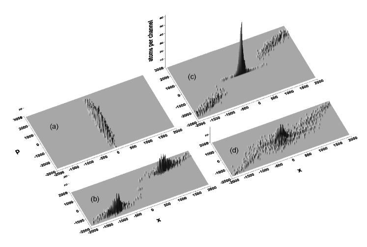
Figure 2: Atomic momentum and position distribution illustrating the effects of atomic acceleration, deceleration, and the velocity grouping: (a) $\tau=0$, (b) $\tau=10^{5}$, $\Delta=-0.2$, (c) $\tau=10^{5}$, $\Delta=0.1$, (d) $\tau=10^{5}$, $\Delta=-0.05$. Momentum $p$ is given in units of $\hbar k_{f}$, the position in units of $k_{f}^{-1}$.

velocity grouping effect at $\Delta=-0.2$ and $\tau=10^{5}$. A large number of atoms is grouped around two values of the capture momentum $p_{\rm cap}\simeq\pm 1300$ because of acceleration of slow atoms and deceleration of the fast ones in the initial ensemble. The slower the atoms are the longer is the process of the velocity grouping. Note that atoms with $|p|\lesssim 100$, trapped initially in a well of the optical potential, could not quit the well up to $\tau=10^{5}$. Contrary to that, at positive values of the detuning fast atoms are accelerated and slow ones are decelerated. As a result, we observe a pronounced peak around $x\simeq p\simeq 0$ shown in Fig. 2c at $\Delta=0.1$ and $\tau=10^{5}$.

Dependence of the friction force $F$ on the current atomic momentum $p$ is shown in Fig. 3 at $\Delta=-0.2$. It has been computed with our main equations (3) when averaging over seven thousands atoms with different initial momentum. The function $F(p)$ resembles the behavior of the friction force computed with another methods

Figure 3: Dependence of the friction force $F\equiv{\lang\dot{p}\rang}$ on the current atomic momentum $p$ at the detuning $\Delta=-0.2$.

(see Kaz and Fig. 1a in PRA05 ). The friction force decreases up to zero value and then begin to oscillate with increasing $p$. It has a number of zeroes (the detailed view is shown in Fig. 3b) like the corresponding functions in Refs. Kaz ; PRA05 . Zero values of $F$ correspond to quasistationary values of the momentum which depend on $\Delta$. Some of them are attractors and atoms with close values of the momentum tend to $p_{\rm cap}$, another ones are repellors. The attractors and repellors are not deterministic because of a random nature of SE. Thus, an atoms walks randomly in the momentum space between different values of the capture momentum $p_{\rm cap}$. When it reaches a certain value of the capture momentum the atom does not stop in the momentum space and goes on to fluctuate because of both the Hamiltonian instability and SE effect.

In the preceding section we described the Hamiltonian chaotic walking that may occur in the absence of any losses. Dissipation causes additional strong fluctuations of the momentum. If $\Delta>0$ or if it is negative but comparatively large, nothing principally new happens to atoms as compared with the Hamiltonian limit. However, at negative small values of $\Delta$, a characteristic capture momentum becomes smaller than a typical range of momentum fluctuations due to atomic recoils. As a result, atoms may change their direction of motion in an irregular way. Such a dissipative chaotic atomic walking is illustrated in Fig. 2d at $\Delta=-0.05$ and $\tau=10^{5}$ with the atoms distributed widely in the phase plane. Typical atomic trajectories are shown in Fig. 4 in the momentum space. Figures 4a and b illustrate how the friction force near the resonance ($\Delta=-0.001$ and $\Delta=-0.01$) decelerates atoms with large values of the initial momentum down to so small values of the capture momentum when the dissipative chaotic walking becomes possible. With increasing the absolute value of the negative $\Delta$, the capture momentum increases and the atom changes rarely the direction of motion (Fig. 4c with $\Delta=-0.1$). Panels d and e in Fig. 4 illustrate the velocity grouping effect at $\Delta=-0.15$ with different values of the initial momentum.

Figure 4: Typical atomic trajectories in the momentum space: (a)-(c) dissipative chaotic walking with different statistics of atomic flights, (d)-(e) the effect of velocity grouping. Note that atoms with very different initial momentum acquire a close value of the capture momentum.

V Statistical properties of dissipative chaotic walking

Statistics of Hamiltonian chaotic walking is quantified by the flight and trapping PDFs (10) with algebraically decaying head segments and exponential tails whose lengths strongly depend on $\Delta$. We will show in this section that PDFs for dissipative chaotic walking are even more sensitive to variations in $\Delta$. Figures 4a and b clearly demonstrate that at very small detuning $\Delta=-0.001$ long flights dominate, whereas there appears a number of short flights with larger value of $\Delta=-0.01$. In Fig. 5 we plot the PDFs $P_{fl}$ for the duration of atomic flights $T$ with different values of the detuning $\Delta$. At small detunings (Fig. 5a), the length of the power-law segments depends on $\Delta$ in a similar way as in the Hamiltonian case (compare this figure with Figs. 5a, 6a, and 7a in Ref. pra07 ). However, the slope slightly differs from the Hamiltonian slope which is equal to $-1.5$. The difference in the statistics of dissipative and Hamiltonian walkings is more evident with larger values of the detuning (Fig. 5b). The length of the power-law segments increases drastically with increasing $\Delta$. This effect is absent in Hamiltonian dynamics. The corresponding slope $\alpha$ decreases with changing the detuning from $\Delta=-0.09$ to $\Delta=-0.12$ because of the corresponding increase in the length of atomic flights (see Figs. 4a, b, and c). In Fig. 6 we plot the dependencies of the mean duration of atomic flights ${\lang T\rang}$ and the slope of the PDF powerlaw fragments $\alpha$ on the detuning $\Delta$ in the range of its medium values $-0.12\leq\Delta\leq-0.06$. Both the quantities correlate well with each other. It means that, changing the value of $\Delta$, one can manipulate statistical properties of dissipative atomic transport in an optical lattice. This control is nonlinear in the sense that slightly changing $\Delta$, say, from $-0.08$ to $-0.12$, we increase the mean duration of flights in a few orders of magnitude. This effect may be qualitatively explained as follows. When increasing the absolute value of the negative detuning, the capture momentum increases but fluctuations of the current momentum $p$ decrease providing long atomic flights epl08 .

To explain the statistical properties of the dissipative chaotic walking let us consider the behavior of the quasienergy

Figure 5: The PDFs $P_{\rm fl}$ for the duration of atomic flights $T$ with (a) small detunings (crosses $\Delta=-0.01$, stars $\Delta=-0.001$, circles $\Delta=-0.0001$, squares $\Delta=-0.00001$) and (b) medium detunings (stars $\Delta=-0.09$, $\alpha=-0.77$; circles $\Delta=-0.1$, $\alpha=-0.27$; squares $\Delta=-0.12$, $\alpha=-0.05$). Straight lines show slopes $\alpha$ of the power-law fragments of the PDFs in log-log scale.

Figure 6: Dependencies of the logarithms of the mean duration of atomic flights $\langle T\rangle$ (solid line) and of the slope $\alpha$ of the PDF power-law fragments (squares) on the detuning $\Delta$ (in units of $\Omega$).

$$\tilde{H}_{j} \equiv\frac{\omega_{r}}{2}p^{2}-u\cos x-\frac{\Delta}{2}z-\frac{\Delta\gamma}{4}{\lang 1-z^{2}\rang}(\tau-\tau_{j})=$$ (12)

$$=H-\frac{\Delta\gamma}{4}{\lang 1-z^{2}\rang}(\tau-\tau_{j}),\quad\tau_{j}<\tau<\tau_{j-1},$$

which is equal to the total atomic energy (5) in the absence of relaxation. Near the resonance, $|\Delta|\ll 1$, $\tilde{H}_{j}$ is almost conserved between SE events, i. e., in the interval $\tau_{j}<\tau<\tau_{j-1}$. The real energy $H$ (see Fig. 1d) decreases a little in between in a linear way. The rate of this decrease is defined by the coefficients of spontaneous emission $\gamma$, the detuning $\Delta$, and the average probability to find the atom in the excited state. Both the quantities, $H$ and $\tilde{H}$, changes abruptly just after SE (because of the corresponding changes in the atomic variables (4)). Just after emitting a $j$th spontaneous photon at $\tau=\tau_{j}$, they have the same values. So, we will model the evolution of the energy as a map $H_{j}\equiv H(\tau_{j}^{+})$ taken at the moments $\tau_{j}^{+}$ just after SE

$$H_{j}=\tilde{H}_{j}-\tilde{H}_{j-1}+H_{j-1}=H_{j-1}+\omega_{r}p(\tau_{j}^{-})\rho_{j}+$$ (13)

$$+\frac{\omega_{r}}{2}\rho_{j}^{2}+\frac{\Delta}{2}+u(\tau_{j}^{-})\cos x(\tau_{j})+$$

$$+\frac{\Delta}{2}z(\tau_{j}^{-})+\frac{\Delta\gamma}{4}{\lang 1-z^{2}\rang}(\tau_{j}-\tau_{j-1}),$$

where the values of the atomic variables $p(\tau_{j}^{-}),u(\tau_{j}^{-})$, and $z(\tau_{j}^{-})$ are taken at the moments $\tau_{j}^{-}$ just before SE. They are, in turn, determined by the coherent evolution between SE.

The stochastic map for the atomic energy (13) provides an important information about the CM motion. It has been shown in Ref. pra07 that atoms move ballistically, if the atomic energy satisfies to the condition $H\gtrsim|u|$, whereas at $H\lesssim|u|$ they may change the direction of motion. The dissipative chaotic walking takes place when the atomic energy $H$ alternatively takes the values larger and smaller than a critical value $H=|u|$. In the Hamiltonian limit, where the energy is conserved, the problem of the CM chaotic walking has been reduced to the task of random walking of the Bloch component $u$ (see Sec. III and Ref. pra07 ). The energy is not conserved in the presence of relaxation, but the values of $u$ are always small (see Appendix and Fig. 1c and d). Thus, atoms oscillate in the wells of the optical potential if $H\lesssim 0$ and move ballistically if $H\gtrsim 0$.

On a time scale exceeding the mean time between SE events $2/\gamma$, the evolution of energy can be treated as a diffusion process with a drift in the energetic space. The probability to have the energy $H$ at time $\tau$ is governed by the Fokker-Planck equation

$$\dot{P}(H,\tau)=-2c_{H}\frac{\partial P}{\partial H}+D_{H}\frac{\partial^{2}P}{\partial H^{2}},$$ (14)

where $D_{H}$ is an energy diffusion coefficient and $c_{H}$ is an energy drift coefficient which can be estimated with the help of Eq. (13) as follows:

$$c_{H}\equiv\frac{{\lang H_{j}-H_{j-1}\rang}}{{\lang\tau_{j}-\tau_{j-}\rang}}={\lang\dot{H}\rang}\simeq\frac{\omega_{r}\gamma}{12}+\frac{\Delta\gamma}{2}.$$ (15)

In deriving this formula we adopt the average value of the squared recoil momentum ${\lang\rho_{j}^{2}\rang}=1/3$ (the projections of the recoil momenta on the standing-wave axis $x$, $\rho_{j}$, are assumed to be distributed in the range $\pm 1$ with the same probability), the average value of the population inversion just before a SE event to be $z(\tau_{j}^{-})=1/2$, the average value of $z$ over the whole time scale and its mean squared deviation from 1 to be ${\lang z\rang}=0$ and ${\lang 1-z^{2}\rang}=1/2$, respectively (see the solution (33) in Appendix). Moreover, neglecting the correlation, we put ${\lang u\cos x\rang}\simeq{\lang u\rang}{\lang\cos x\rang}=0$, which is valid if $|\omega_{r}p|\gtrsim\gamma/2$, i. e., when $p\gtrsim 100$ with our choice of the parameters. Since the first term in (15) is small and may be neglected, the drift velocity of an atom in the energetic space is approximately proportional to the detuning $\Delta$, and, therefore in average atoms accelerate and decelerate at $\Delta>0$ and $\Delta<0$, respectively, as it should be for $|\Delta|\ll 1$. In the weak Raman-Nath approximation, (32) and (34), the drift coefficient in the energetic space is simply related to the friction force $F$ acting upon atoms

$$F\equiv{\lang\dot{p}\rang}\simeq\frac{{\lang\dot{H}\rang}}{\omega_{r}p}.$$ (16)

The friction force plays the role of a drift coefficient in the momentum space. Strictly speaking, the weak Raman-Nath approximation is not valid near the turning points when the atomic velocity is comparatively small. However, most of the flight time it is valid.

The diffusion coefficient in the energetic space is given by the formula

$$\ D_{H}\equiv\frac{{\lang(H_{j}-H_{j-1})^{2}\rang}-{\lang H_{j}-H_{j-1}\rang}^{2}}{2{\lang\tau_{j}-\tau_{j-1}\rang}},$$ (17)

which can be rewritten with the help of (13) as follows:

$$D_{H}\simeq\frac{\gamma\omega_{r}^{2}p^{2}(\tau_{j}^{-})}{{12}}+\frac{{\lang u^{2}(\tau_{j}^{-})\rang}\gamma}{8}.$$ (18)

Using weak Raman-Nath approximation, (32) and (34), the first term can be replaced by $\gamma\omega_{r}H/6$. Using the estimation (38) for ${\lang u^{2}(\tau_{j}^{-})\rang}$ in the irregular CM motion regime (see Appendix), we get the following expression for the energy diffusion coefficient:

$$D_{H}^{ch}\simeq\frac{\gamma\omega_{r}H}{{6}}+\frac{\Delta^{2}}{8}.$$ (19)

This expression is valid for moderately small momentums ($p\lesssim 1000$) when the strong Raman-Nath approximation cannot be applied. In the process of dissipative chaotic walking, the probability to get higher values of the momentums is almost zero.

Now we will try to derive analytically a distribution of the durations $T$ of atomic flights in the process of dissipative chaotic walking. In fact, it is a problem of the first passage time for the atomic energy $H$ to return to its zero value. Recall that at small detunings we have $H\simeq 0$ in the very beginning of every flight. In course of time $H$ can reach rather large values, and it returns to zero at the end of the flight. If the random jumps of the energy would be symmetric ($c_{H}=0$), the probability to find a flight with duration $T$ would be proportional to $T^{-1.5}$, where the exponent $-1.5$ does not depend on the diffusion coefficient. This conjecture follows from the known theorem in probability theory. More general result (see chapter XIV in Ref. Feller ) proves that in the case of an asymmetric random walking in the energetic space ($c_{H}\neq 0$) the PDF for the flight durations in configuration space is

$$P_{\rm{fl}}\propto e^{-c_{H}^{2}T/D_{H}}T^{-1.5},$$ (20)

if the drift and diffusion coefficients in the Fokker-Planck equation for the random walking are assumed to be constants. This formula gives a distribution of the flight durations with a power-law fragment followed by an exponential tail and agrees qualitatively with the exact numerical computations of $P_{fl}$ shown in Fig. 5a for a few values of the detuning $\Delta$. The main disadvantage of this formula is that (20) does not depend on $\Delta$ as the exact PDFs in Fig. 5a. At very small $\Delta=-10^{-5}$, the PDF, shown by squares in Fig. 5a, decays mostly algebraically, whereas at larger values of the detuning the power-law fragments are much shorter. A discrepancy between the analytical and numerical PDFs arises because we assumed in deriving (20) that $D_{H}$ and $c_{H}$ do not depend on the energy $H$. In fact, it is not the case for small values of the momentum $p$, and a more accurate formula for $P_{fl}(T)$ is required.

The PDFs for Hamiltonian (10) and dissipative (20) transport are similar in the sense that both $P_{fl}$ contain power-law fragments followed by exponential tails, but the origin of each statistics is different. In the Hamiltonian limit the statistics is governed by the behavior of $u$, not the energy, as in the dissipative system. A turnover from a power law to an exponential decay in the Hamiltonian case is explained by a boundedness of $|u|\lesssim 1$, whereas in the dissipative system it is explained by a negative drift of the energy $H$. Each of the factors prevents the corresponding randomly walking quantity to go far away from its critical value (at which the atoms can change the directions of motion) decreasing the probability of long flights in at exponential way.

VI Manifestation of Hamiltonian chaos in dissipative atomic transport

In the absence of SE the atomic dynamics can be regular or chaotic depending on the initial conditions and/or the detuning. In experiments one measures statistical characteristics of spontaneously emitting atoms. Is there a correlation between those characteristics and the underlying Hamiltonian dynamics? Can we find any manifestations of Hamiltonian instability, chaos, and order, in the diffusive-like dissipative atomic transport? These questions will be addressed in the present section.

The common quantitative criterion of deterministic chaos, the maximal Lyapunov exponent $\lambda$, is a measure of a divergence of two trajectories in the phase space with close initial conditions LL83 . To quantify probability of chaos in the mixed Hamiltonian dynamics, when $\lambda=0$ with some values of $p_{0}$ and $\lambda>0$ with another values of $p_{0}$, we introduce a probabilistic measure of Hamiltonian chaos

$$\Lambda\equiv{\lang 2\Theta(\lambda)-1\rang},$$ (21)

where $\Theta(\lambda)$ is a Heaviside function ($\Theta=0$ if $\lambda<0$, $\Theta=1/2$ if $\lambda=0$, and $\Theta=1$ if $\lambda>0$). The probability of Hamiltonian chaos $\Lambda$ is computed by averaging over a large number of atomic trajectories with different values of $p_{0}$. If all the trajectories in the set turn out to be stable, one gets $\Lambda=0$, and if all they are exponentially unstable, then $\Lambda=1$. One gets $0<\Lambda<1$, if some trajectories in the set are stable but the other ones are not. The magnitude of $\Lambda$ is proportional to the fraction of trajectories with positive $\lambda$s.

To examine manifestations of the underlying Hamiltonian dynamics in dissipative transport in is convenient to consider atomic diffusion not in the energetic but in the momentum space. The momentum diffusion coefficient, which is a measure of momentum fluctuations, can be written with the help of (17) and (32) as follows:

Figure 7: Correlation between the average momentum diffusion coefficient in a log-log scale $D_{p}$ (in units of $\hbar^{2}k^{2}_{f}\Omega$) and probability of Hamiltonian chaos $\Lambda$ in their dependencies on current atomic momentum $p$ (in units of $\hbar k_{f}$) at $\Delta=-0.01$ and $\Delta=-0.0005$. Dashed lines with the slopes $~{}p^{-2}+{\rm const}$ and $~{}p^{-1}+{\rm const}$ are theoretical curves (23) and (24) valid in the regimes of Hamiltonian chaos and order, respectively. Solid line is a theoretical curve (25) derived to fit the exact numerical results. An abrupt change in the decay laws for $D_{p}$ occurs for those values of $p$ where the transition from order to chaos takes place in the underlying Hamiltonian dynamics.

$$D_{p}\simeq\frac{D_{H}}{\omega_{r}^{2}p^{2}}\simeq\frac{\gamma}{{12}}+\frac{{\lang u^{2}(\tau_{j}^{-})\rang}\gamma}{8\omega_{r}^{2}p^{2}}.$$ (22)

Using the formula (19), we get $D_{p}$ in the regime of chaotic oscillations of the Bloch component $u$

$$D_{p}^{ch}\simeq\frac{\gamma}{{12}}+\frac{\Delta^{2}}{8\omega_{r}^{2}p^{2}}.$$ (23)

The momentum diffusion coefficient $D_{p}$ is computed with the main equations (3) in the following way. The range of all possible values of the atomic energy $H$ (5) is partitioned in a large number of bins. For a large number of initial conditions (in fact, we change only the initial momentum $p_{0}$ keeping the other conditions to be fixed), after any $j$th SE event we compute the difference $H_{j}-H_{j-1}$ and the squared difference $(H_{j}-H_{j-1})^{2}$. They are random values, but their statistics depend on the preceding energy value $H_{j-1}$. So we calculate the histograms of the average values of ${\lang H_{j}-H_{j-1}\rang}$ and ${\lang(H_{j}-H_{j-1})^{2}\rang}$ as functions of energy $H_{j-1}$. After that we can compute the energy diffusion coefficient $D_{H}$ (17) which, being divided by $\omega_{r}^{2}p^{2}$, yields the momentum diffusion coefficient $D_{p}$ which is better to present as a function of the current momentum $p\simeq\sqrt{2H_{j-1}/\omega_{r}}$.

The main result in this section is illustrated with Fig. 7. In the upper left and right panels the dependencies of the momentum diffusion coefficient $D_{p}$ on the current momentum $p$ are plotted in a log-log scale for $\Delta=-0.01$ and $\Delta=-0.0005$, respectively. In both the cases, we put $\gamma=0.0033$. These plots should be compared with the corresponding lower panels where the probability of the Hamiltonian chaos $\Lambda$ is plotted against $p$ with $\gamma=0$ (i. e. in the Hamiltonian limit of Eqs. (3)). It is evident that the character of the momentum diffusion changes abruptly at those values of the current momentum where a transition from chaos to order occurs in the underlying Hamiltonian dynamics. Such a turnover takes place in a range of small negative detunings and is a manifestation of the peculiarities of the underlying Hamiltonian evolution in the diffusive-like dissipative transport of atoms in a standing-wave laser field. We may conclude that in spite of random atomic recoils due to SE the chaotic (regular) dynamics between the acts of SE clearly manifests itself in the behavior of the measurable characteristic of the atomic transport, the momentum diffusion coefficient $D_{p}$. The behavior of $D_{p}$ in the range of $p$, where the underlying Hamiltonian evolution is chaotic, is well described by the formula (23) with $D_{p}^{ch}\sim p^{2}+const$ (see both the upper panels in Fig. 7 where this dependence is shown by dashed lines).

However, the formula (23) does not work in the regimes when the underlying Hamiltonian dynamics is mixed or regular because in deriving it we supposed fully chaotic behavior of $u$. We have managed to estimate analytically $D_{p}$ in the Hamiltonian regular regime at extremely small values of the detuning $|\Delta|\lll 1$ and for atoms whose momentum is so large that we can neglect its fluctuations between SE events (the exact Raman-Nath approximation with $x=\omega_{r}p\tau$). Figure 1a illustrates the ladder-like behavior of $u$ which is descibed by the deterministic mapping (8) on a comparatively short timescale. To get $D_{p}^{RN}$ from Eq. (22) we use the expression (37) for $u^{2}(\tau_{j}^{-})$ derived in Appendix

$$D_{p}^{RN}\simeq\frac{\gamma}{{12}}+\frac{\Delta^{2}}{8\omega_{r}p\gamma\pi}.$$ (24)

Thus, we derived the formulas for the momentum diffusion coefficient $D_{p}$ in the regimes of Hamiltonian chaos (23) with $\Lambda=1$ and Hamiltonian order (24) with $\Lambda=0$. In a general case with $0\leq\Lambda\leq 1$, we will assume a linear combination

$$D_{p}\simeq(1-\Lambda)D_{p}^{RN}+\Lambda D_{p}^{ch}\simeq$$ (25)

$$\simeq\frac{\gamma}{{12}}+\frac{\Delta^{2}}{8\omega_{r}p}\left(\frac{1-\Lambda}{\gamma\pi}+\frac{\Lambda}{\omega_{r}p}\right).$$

This function, shown by the solid line in the right upper panel in Fig. 7, fits rather well exact numerical results.

We would like to end this section with the proposal of a simple experimental scheme to observe our main theoretical and numerical result on an abrupt change in the character of atomic diffusion in a laser standing wave under conditions corresponding to two different regimes of the underlying Hamiltonian evolution, chaotic and regular ones. Let us consider a small atomic cloud moving in one direction with an average atomic momentum ${\lang p_{c}\rang}$. Initial position and momentum distribution are assumed to be a Gaussian with the standard deviations $\sigma^{2}_{x}\equiv{\lang(x-{\lang x_{c}\rang})^{2}\rang}$ and $\sigma^{2}_{p}\equiv{\lang(p-{\lang p_{c}\rang})^{2}\rang}$. The momentum diffusion coefficient is

$$D_{p}=\frac{d(\sigma^{2}_{p})}{2d\tau}.$$ (26)

The temperature of gas and its rate of heating in Kelvins per second are

$$T\equiv\frac{2{\lang E_{k}\rang}}{k_{B}}=\frac{\hbar^{2}k^{2}_{f}\sigma^{2}_{p}}{m_{a}k_{B}},\quad\frac{dT}{dt}=\frac{2\hbar^{2}k^{2}_{f}\Omega D_{p}}{m_{a}k_{B}},$$ (27)

where $E_{k}$ is a kinetic energy of atoms (in Joules) in the reference frame moving with the CM of the cloud. It follows from (27) that the rate of heating is proportional to $D_{p}$ whose behavior is different in the regimes of regular and chaotic underlying Hamiltonian dynamics.

The linear extent of the cloud in meters is $L_{X}\equiv 2\sigma_{x}/k_{f}$. On a comparatively short time scale, $\tau\ll|({\lang p_{c}\rang}/F)|$, and low temperatures $\sigma_{p}\ll|{\lang p_{c}\rang}|$, $D_{p}$ is approximately the same for all the atoms in the cloud because the CM velocity could not change significantly under the action of the friction force $F$ during the observation time. Using the first equation in the set (3) and the Eq.(26), we obtain

$$\sigma^{2}_{x}\simeq\sigma^{2}_{x}(0)+\frac{1}{2}\omega^{2}_{r}\sigma^{2}_{p}(0)\tau^{2}+\frac{2}{3}D_{p}\omega^{2}_{r}\tau^{3}.$$ (28)

Figure 8: A log-log dependence of the cloud’s linear extent $L_{X}$ (in microns) on the average initial momentum ${\lang p_{c}\rang}$ of atoms in a cloud at two moments of time. The analytic dashed lines were computed with the formula (28) with $D_{p}=D_{p}^{ch}$ valid in the chaotic regime on a short time scale. Note an abrupt change in the decay of $L_{X}({\lang p_{c}\rang})$ in the range of ${\lang p_{c}\rang}\simeq 1200$ where a chaos-order transition takes place in the underlying Hamiltonian motion. $\Delta=-0.01$, $2\sigma_{x}(0)=0.5$, $2\sigma_{p}(0)=5$, wavelength $\lambda_{f}=2\pi/k_{f}=850$ nm.

We have computed $L_{X}$ with that formula with $D_{p}$ given by (23) and compare the result with numerical simulation of Eqs. (3) for a number of atomic clouds with different initial values of ${\lang p_{c}\rang}$. In Fig. 8 the dependence $L_{X}({\lang p_{c}\rang})$ is plotted for $\Delta=-0.01$ at two moments of time. The analytic dashed lines fit well the exact numerical results in the range ${\lang p_{c}\rang}\lesssim 1200$ where the underlying Hamiltonian dynamics is chaotic (see the left column in Fig. 7). Note an abrupt change in the decay of $L_{X}({\lang p_{c}\rang})$ beginning with those values of ${\lang p_{c}\rang}\simeq 1200$ where the Hamiltonian dynamics becomes more regular. Since the linear extent of the atomic clouds changes abruptly at the chaos-order border one may conclude that in real experiments the value of $L_{X}$ should increase sharply with those values of the average cloud momentum ${\lang p\rang}$ for which the underlying Hamiltonian evolution is chaotic.

VII Conclusion

Coherent evolution of the atomic state in a near-resonant standing-wave laser field is interrupted by SE events at random moments of times. The Hamiltonian evolution between these events has been shown previously (for a summary of Hamiltonian theory for cold atoms in a 1D optical lattice see Ref. pra07 ) to be regular or chaotic depending on the values of the detuning $\Delta$ and the initial momentum $p_{0}$. We stress that dynamical chaos may happen without any noise and any modulation of the lattice parameters. It is a specific kind of dynamical instability in the fundamental interaction between the matter and radiation.

In reality Hamiltonian chaos is masked by random events of SE. The behavior of spontaneously emitting atoms in the detuning and momentum regimes where the underlying Hamiltonian dynamics is chaotic may be called stochastic chaos. We have specified and quantified two regimes of the stochastic chaos, namely, random walking and dissipative ballistic transport. In the first regime, atoms wander in an optical lattice in a random way performing flights in both the directions with the PDFs strongly depending on the detuning (see Figs. 5 and 6). In the ballistic regime, atoms move in the same direction with momentum fluctuations caused both by the Hamiltonian instability as well as SE events. It has been shown in our numerical experiments and confirmed analytically that the character of momentum diffusion changed abruptly in the regime where the underlying Hamiltonian dynamics proved to be chaotic. A clear correlation between the decay of the momentum diffusion coefficient $D_{p}$ and probability of Hamiltonian chaos $\Lambda$ has been found (Fig. 7). In order to observe the manifestation of Hamiltonian chaos in real experiments we proposed to measure a linear extent of atomic clouds $L_{X}$ in a 1D optical lattice and predicted a significant increase in $L_{X}$ for the atomic clouds with $\Lambda\simeq 1$.

In conclusion we would like to discuss some possible applications of the theory developed and the results obtained. A sensitive dependence of statistical properties of dissipative chaotic walking and ballistic transport on the values of the detuning $\Delta$ provides a possibility to manipulate atomic CM motion by changing $\Delta$. For example, one can increase the mean duration of atomic flights in three orders of magnitude by changing $\Delta$ only by thirty percents (see Fig. 6).

Cold atoms in optical lattices is an ideal system to study different phenomena in statistical physics. Besides dynamical chaos, the phenomena of stochastic resonance has been observed in a near-resonant optical lattice SC02 . Another phenomenon of considerable current interest is cold atom ratchets ML99 ; SS03 ; JG04 ; GB07 ; GP07 . A ratchet is a spatially periodic device which is able to produce a directed transport of particles in the absence of a net bias (i. e., when the time- and space-averaged forces are zero). In order to realize the ratchet effect it is necessary to break time or/and spatial symmetries which generate a countermoving partner to each trajectory FY00 . Different classes of the ratchets have been experimentally realized with cold atoms in optical lattices ML99 ; SS03 ; JG04 . The interrelation of Hamiltonian chaos and SE noise, found in this paper, provides an additional possibility to create and manipulate directed transport of atoms in rigid optical lattices.

Appendix

We work in the regime of small detunings

$$|\Delta|\ll 1,$$ (29)

moderate mean atomic velocities

$${\lang|\omega_{r}p|\rang}\sim\gamma/2\ll 1,$$ (30)

and diffusive motion

$$\tau\gg 2/\gamma.$$ (31)

Due to (29), we may neglect the last term in the potential energy (5) and adopt the Hamiltonian solutions for (7) between any two acts of SE. The evolution of $u$ is described by the approximate solutions (8) for the regular Raman-Nath motion and (9) for the chaotic motion. It follows from the condition of moderate atomic velocity (30) and solutions (8), (9) that $|u|\ll 1$. In other words, $u$ cannot go far from zero between acts of SE after each of which $u=0$. Under the conditions (29) and $|u|\ll 1$, the mean kinetic atomic energy is much greater than the potential one and in this weak Raman-Nath approximation

$$|u\sin x+\frac{\Delta z}{2}|\ll\frac{\omega_{r}p^{2}}{2},$$ (32)

the solution (7) for $z$ is simplified

$$z(\tau)\simeq\mp\sin\left(2\int\limits_{0}^{\tau}\cos xd\tau^{\prime}+\chi_{0}\right).$$ (33)

In the diffusion regime (31) and in the weak Raman-Nath approximation (32) the momentum fluctuations between two SE are small in comparison with its fluctuations over the time scale of atomic transport. So, the atomic momentum just before SE is equal to its value at the node

$$p\simeq p(\tau_{j}^{-})\simeq p_{\rm node}.$$ (34)

Now we can get simplified solutions for $u$. In the exact Raman-Nath condition, $x=\omega_{r}p\tau$, we have from (8) the approximate deterministic map written in a two-step form

$$u_{m}^{RN}\approx 2\Delta\sqrt{\frac{\pi}{\omega_{r}p}}\ v_{0}\cos\left(\frac{2}{\omega_{r}p}-\frac{\pi}{4}\right)+u_{m-2}^{RN}.$$ (35)

In the chaotic regime we have from $(\ref{u_m})$ the stochastic map

$$u_{m}^{ch}=|\Delta|\sqrt{\frac{\pi}{\omega_{r}p}}\sin\phi_{m}+u_{m-1}^{ch}.$$ (36)

The maps derived enable us to estimate the values of $u(\tau_{j}^{-})$ just before $j$th act of SE. After the $(j-1)$th SE $u_{0}=u(\tau_{j-1}^{+})=0$, $u(\tau_{j}^{-})=u_{M}$ is an accumulated value of $u$ after passing $M$ nodes in the interval $\tau_{j-1}<\tau<\tau_{j}$. The average number of node crossings can be estimated to be ${\lang M\rang}\simeq 2|\omega_{r}p|/\gamma\pi$. In the exact Raman-Nath limit, $u_{M}=M(u_{m}-u_{m-2})/2$, and the mean squared value in the regular regime

$${\lang u^{2}(\tau_{j}^{-})\rang}_{RN}={\lang u^{2}_{M}\rang}_{RN}\simeq\frac{4\Delta^{2}\omega_{r}p}{\pi\gamma^{2}}\ {\lang v^{2}_{0}\rang}\cos^{2}\left(\frac{2}{\omega_{r}p}-\frac{\pi}{4}\right).$$ (37)

Beyond the strong Raman-Nath limit, $u(\tau_{j}^{-})=u_{M}$ is a sum of $M$ random numbers which are proportional to $\sin\phi_{m}$. From the probability theory we get

$${\lang u^{2}(\tau_{j}^{-})\rang}_{ch}={\lang u^{2}_{M}\rang}_{ch}\simeq{\lang M\rang}\Delta^{2}\frac{\pi}{2\omega_{r}p}\simeq\frac{\Delta^{2}}{\gamma}.$$ (38)

References

- (1) V. G. Minogin and V. S. Letokhov, Laser Light Pressure on Atoms (New York, Gordon and Breach, 1987).
- (2) A. P. Kazantsev, G. I. Surdutovich, and V. P. Yakovlev, Mechanical Action of Light on Atoms (Singapore, World Scientific, 1990).
- (3) P. Meystre, Atom Optics (New York, Springer-Verlag, 2001).
- (4) G. Grynberg and C. Robilliard, Phys. Rep. 355, 335 (2001).
- (5) O. Morsch and M. Oberthaler, Rev. Mod. Phys. 78, 179 (2006).
- (6) F. L. Moore, J. C. Robinson, C. Bharucha, P. E. Williams, and M. G. Raizen, Phys. Rev. Lett. 73, 2974 (1994).
- (7) J. C. Robinson, C. Bharucha, F. L. Moore, R. Jahnke, G. A. Georgakis, Q. Niu, M. G. Raizen, and Bala Sundaram, Phys. Rev. Lett. 74, 3963 (1995).
- (8) S. Dyrting and G. J. Milburn, Phys. Rev. A 51, 3136 (1995).
- (9) H. Ammann, R. Gray, I. Shvarchuck, and N. Christensen, Phys. Rev. Lett. 80, 4111 (1998).
- (10) J. Ringot, P. Szriftgiser, J. C. Garreau, and D. Delande, Phys. Rev. Lett. 85, 2741 (2000).
- (11) T. M. Fromhold et al, J. Opt. B: Quantum Semiclass. Opt. 2, 628 (2000).
- (12) W. K. Hensinger et al, J. Opt. B: Quantum Semiclass. Opt. 5, R83 (2003).
- (13) P. H. Jones, M. M. Stocklin, G. Hur, and T. S. Monteiro, Phys. Rev. Lett. 93, art. 223002 (2004).
- (14) R. Graham, M. Schlautmann, and P. Zoller, Phys. Rev. A 45, R19 (1992).
- (15) B. G. Klappauf, W. H. Oskay, D. A. Steck, and M. G. Raizen, Phys. Rev. Lett. 81, 1203 (1998).
- (16) G. H. Ball, K. M. D. Vant, H. Ammann, N. L. Cristensen, J. Opt. B: Quantum Semiclass. Opt. 1, 357 (1999).
- (17) D. A. Steck, V. Milner, W. H. Oskay, and M. G. Raizen, Phys. Rev. E 62, 3461 (2000).
- (18) M. B. d’Arcy et al, Phys. Rev. E 64, 056233 (2001).
- (19) D. A. Steck et al, Science 293 274 (2001).
- (20) W. K. Hensinger et al, Nature 412 52 (2001).
- (21) D. A. Steck, W. H. Oskay, and M. G. Raizen, Phys. Rev. Lett. 88 120406 (2002).
- (22) S. Chu, L. Hollberg, J. E. Bjorkholm, A. Cable, and A. Ashkin, Phys. Rev. Lett. 55, 48 (1985).
- (23) F. Bardou, J. P. Bouchaud, A. Aspect, and C. Cohen-Tannoudji, Lévy Statistics and Laser Cooling (Cambridge University Press, Cambridge, 2002).
- (24) F. Bardou, J.P. Bouchaud, O. Emile, A. Aspect, and C. Cohen-Tannoudji, Phys. Rev. Lett. 72, 203 (1994).
- (25) C. Jurczak et al, Phys. Rev. Lett. 77, 1727 (1996).
- (26) H. Katori, S. Schlipf, and H. Walther, Phys. Rev. Lett. 79, 2221 (1997).
- (27) S. Marksteiner, K. Ellinger, and P. Zoller, Phys. Rev. A 53, 3409 (1996).
- (28) S. V. Prants and V. Yu. Sirotkin, Phys. Rev. A 64, art. 033412 (2001).
- (29) S. V. Prants and L. E. Kon’kov, JETP Lett. 73, 180 (2001) [Pis’ma ZhETF 73, 200 (2001)].
- (30) S. V. Prants, JETP Letters 75, 651 (2002) [Pis’ma ZhETF 75, 777 (2002)].
- (31) V. Yu. Argonov and S. V. Prants, JETP 96, 832 (2003) [Zh. Eksp. Teor. Fiz. 123, 946 (2003)].
- (32) S. V. Prants and M. Yu. Uleysky, Phys. Lett. A 309, 357 (2003).
- (33) V. Yu. Argonov and S. V. Prants, Phys. Rev. A 75, art. 063428 (2007).
- (34) S. V. Prants, M. Edelman, and G. M. Zaslavsky, Phys. Rev. E 66, art. 046222 (2002).
- (35) V. Yu. Argonov and S. V. Prants, J. Russ. Laser Res. 27, 360 (2006).
- (36) H. J. Carmichael, An open systems approach to quantum optics (Berlin, Springer, 1993).
- (37) J. Dalibard, Y. Castin, and K. Mölmer, Phys. Rev. Lett. 68, 580 (1992).
- (38) R. Dum, P. Zoller, and H. Ritsch, Phys. Rev. A 45, 4879 (1992).
- (39) S. V. Prants, JETP Lett. 75, 63 (2002) [Pis’ma ZhETF 75, 71 (2002)].
- (40) C.J. Hood, T.W. Lynn, A.C. Doherty et al, Science 287, 1447 (2000).
- (41) V. Yu. Argonov and S. V. Prants, Phys. Rev. A 71, 053408 (2005).
- (42) V. Yu. Argonov and S. V. Prants, Acta Phys. Hung. B 26, 121 (2006).
- (43) V. Yu. Argonov and S. V. Prants, Europhys. Lett. 81, 24003 (2008).
- (44) W. Feller, An Introduction to Probability Theory and its Applications (New York, John Wiley & Sons, Inc., 1964).
- (45) A. J. Lichtenberg, M. A. Lieberman, Regular and Stochastic Motion (Springer, New York, 1983).
- (46) L. Sanchez-Palencia, F. R. Carminati, M. Schiavoni, F. Renzoni, and G. Grynberg, Phys. Rev. Lett. 88, 133903 (2002).
- (47) C. Mennerat-Robilliard et al, Phys. Rev. Lett. 82, 851 (1999).
- (48) M. Schiavoni, L. Sanchez-Palencia, F. Renzoni, and G. Grynberg, Phys. Rev. Lett. 90, 094101 (2003).
- (49) P. H. Jones, M. Goonasekera, and F. Renzoni, Phys. Rev. Lett. 93, 073904 (2004).
- (50) R. Gommers, M. Brown, and F. Renzoni, Phys. Rev. A 75, 053406 (2007).
- (51) J. Gong, D. Poletti, and P. Hanggi, Phys. Rev. A 75, 033602 (2007).
- (52) S. Flach, O. Yevtushenko, and Y. Zolotaryuk, Phys. Rev. Lett. 84, 2358 (2000)