Uncovering the Birth of a Coronal Mass Ejection from Two-Viewpoint SECCHI Observations

Abstract

We investigate the initiation and formation of Coronal Mass Ejections (CMEs) via detailed two-viewpoint analysis of low corona observations of a relatively fast CME acquired by the SECCHI instruments aboard the STEREO mission. The event which occurred on January 2, 2008, was chosen because of several unique characteristics. It shows upward motions for at least four hours before the flare peak. Its speed and acceleration profiles exhibit a number of inflections which seem to have a direct counterpart in the GOES light curves. We detect and measure, in 3D, loops that collapse toward the erupting channel while the CME is increasing in size and accelerates. We suggest that these collapsing loops are our first evidence of magnetic evacuation behind the forming CME flux rope. We report the detection of a hot structure which becomes the core of the white light CME. We observe and measure unidirectional flows along the erupting filament channel which may be associated with the eruption process. Finally, we compare these observations to the predictions from the standard flare-CME model and find a very satisfactory agreement. We conclude that the standard flare-CME concept is a reliable representation of the initial stages of CMEs and that multi-viewpoint, high cadence EUV observations can be extremely useful in understanding the formation of CMEs.

1 Introduction

sec:Introduction

CMEs have been observed for more than 40 years now. They are one of the most energetic phenomena in our solar system and the main driver of disturbances in the terrestrial space environment. Despite observations of tens of thousands of CMEs, the physical processes behind their formation and propagation have not yet been understood completely [Klimchuk (2001), Forbes et al. (2006), Chen (2011)].

To make progress, we need to select the model (or models) that best describe the phenomenon. To accomplish this, it is necessary to test the theoretical predictions of the various models against the observations as was discussed by 2001AGUGM.125..143K. Here, we concentrate on the ’standard’ flare-CME model, also known as the CSHKP model [Švestka and Cliver (1992)]. This is not actually a fully-fledged model derived from the solution of a set of Magnetohydrodynamic (MHD) equations but it is rather a two-dimensional (2D) cartoon representation of the erupting process. However it captures the key ingredients of many MHD models (i.e., the three-part CME, the ejection of a flux rope, post-CME flaring loops, etc) and demonstrates, in a straightforward way, the possible connection between the erupting and flaring processes. For our discussion, we use the detailed model representation in 2004ApJ…602..422L (their Figure 1) but many more variations can be found in the literature.

Even as a cartoon, the CSHKP model makes several predictions that can be tested against the observations. First, it predicts the eruption of a core surrounded by a cavity (or bubble) that forms during the initiation process. High temperatures are expected in both the cavity and the core as result of magnetic reconnection [Chen (2011)]. Second, the reconnection behind the erupting system creates a magnetic void which draws adjacent lines toward the current sheet thereby creating an inflow of material from the surrounding flux systems. Third, through the reconnection processes in the post-CME current sheet, magnetic energy is transformed into thermal energy that powers the flare and kinetic energy that powers the CME. Therefore, we expect a close correspondence between the SXR light curve and the CME acceleration profile as has been found in the past (e.g., 2004ApJ…604..420Z). A delay between the two processes is also likely depending on the magnetic fields and reconnection rates involved [Reeves (2006)]. Fourth, there are many candidates for the role of the eruption trigger. Flux emergence, tether-cutting or even mass unloading from the prominence channel, are all capable of driving the system out of its equilibrium state to set off the eruption (see discussion and references in 2011LRSP….8….1C). Can the trigger be identified in the observations?

Many, if not all, of these predictions relate to the very first stages of the CME; namely, its initiation and formation. However, the initiation and formation stages of CMEs present some serious observational challenges. The CME formation and initial evolution take place low in the corona which is accessible only to imagers in the Extreme Ultraviolet (EUV) or (less often) Soft X-Ray (SXR) wavelengths. These instruments observe in a relatively narrow passband and hence are sensitive to only a narrow range of temperatures, at a time. CME triggers, such as plasma instabilities occur within Alfvenic temporal and spatial scales (of the order of tens of seconds or hundreds of km for an active region). The subsequent energy release also occurs in similar scales and the eruption is usually accompanied by other phenomena such as flares, jets and lateral plasma motions that may have nothing to do with the erupting structure but they complicate the interpretation of the EUV observations.

Therefore, we need observations of the formation stages of a CME taken with high cadence and spatial resolution but with minimal line-of-sight confusion. The unique stereoscopic viewing and instrument complement provided by the Sun-Earth Connection Coronal and Heliospheric Investigation (SECCHI; 2008SSRv..136…67H) on-board the Solar TErrestial RElations Observatory (STEREO) [Kaiser et al. (2008)] fulfills these requirements nicely.

To demonstrate this, we undertake a CME initiation study for an event which took place on January 2, 2008. The eruption in the low corona was observed very well by both SECCHI Extreme Ultraviolet Imagers (EUVI). We are able to examine in detail the various stages of the initiation of a CME and relate them to the usual phenomena that accompany these eruptions, such as flares and filament ejections. In addition, we capture the transition of loop arcades into the forming flux rope and report the first three-dimensional observations of loop ’implosion’. Taken together, these observations reveal many of the key components of CME initiation and provide strong constraints for CME models. The paper is organized as follows. In Section 2, we present the time history of the CME and discuss in detail several key observations including the close correspondence between the acceleration profile and the GOES SXR light curve, the novel observation and 3D measurements of collapsing loops, the detection of a hot CME core, and the observation of outflows along the filament channel. We conclude in Section 3.

2 Stereoscopic Observations of the January 2, 2008 CME

The event under study erupted from active region NOAA 10980 located at S05E65 (Figure fig:context). The region has an alpha magnetic configuration with a single leading negative polarity sunspot. The sunpot disappeared within a couple of days leaving only an extended area of plage fields. The eruption occurred along a filament channel (thick white line in Figure fig:context) overlying a neutral line extending from the center of the region to its periphery. The CME was accompanied by a GOES C1.2 flare starting at 06:51 UT, peaking at 10:00 UT, and ending at 11:21 UT. It is therefore a long duration Soft X-ray (SXR) event but the gradual rise of the light curve is also indicative of a partially occulted event. Indeed, upward motions at the location of the subsequent CME can be detected much earlier than the flare peak as we shall see later. The event was observed by the SECCHI/EUVI imagers on the STEREO-A and STEREO-B spacecraft which were located $21^{\circ}$ West and $23^{\circ}$ East from the Sun-Earth line, respectively. Therefore, it was a limb event for EUVI-A ($\sim 88^{\circ}$) and an eastern event for EUVI-B ($\sim 42^{\circ}$). The 3D kinematics of the CME in the SECCHI coronagraph fields of view have been discussed in detail by [Zhao et al. (2010)]. Here, we focus on the initiation of the CME in the low corona as witnessed in the EUVI fields of view up to about 1.7 R_sun. We use mainly the 171Å images because of their high cadence (150 sec) but we discuss the observations in the other wavelengths as well. The images have been processed by the 2008ApJ…674.1201S wavelet-based algorithm to enhance the visibility of the off-limb structures by removing the instrumental stray light.

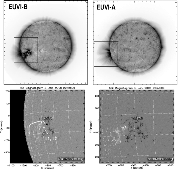
Figure 1.: Top panels: EUVI-A and -B 171Å full disk images on January 2, 2008 at 09:01 UT. The box marks the FOV around AR 10980 used in the subsequent analysis. Bottom panels: MDI magnetograms of AR10980 on January 2 and 4 showing the magnetic field configuration for the event. The thick white line marks the filament channel involved in the eruption. The arrow mark the approximate location of collapsing loops discussed in sec:collapsing. The magnetogram images are courtesy of SolarMonitor.org. fig:context

2.1 The time history of the CME formation in the low corona

Because of the unusual duration of the eruption, we have to find a reliable marker for the start of the event. We use the time of the first unambiguous detection of upward motion of EUV loops at the location of the subsequent CME. This occurs at 06:13:30 UT (online movie and Figure fig:detail). We rely on the EUVI-A images to describe the upward evolution since the CME is propagating along the sky plane of STEREO-A and therefore the images are least affected by projection effects.

The motion in EUVI-A originates in a high-lying loop system which appears to encompass a cavity as evidenced by the lack of 171Å emission (Figure fig:detail). Inside this cavity (in projection) we detect a single bright loop (L1) that begins to collapse as the rest of the loop system expands slowly. The loop is visible from 05:33:30 UT to 07:21:00 UT. The behavior of this collapsing loop is almost immediately imitated by a larger loop arcade (L2). Their collapse starts at around 08:18:30 UT. The CME front leaves the edge of the EUVI-A field of view at 09:18:30 UT. The first evidence of a CME core, in the traditional sense of a 3-part CME, becomes apparent at 09:15:30 UT while the L2 system continues to collapse. At 10:03:30 UT, the loop arcade disappears, the CME continues to accelerate and the usual post-eruptive arcade forms. An EUV wave is launched by the expanding CME at around 10:33:30 UT. Material continues to flow outward from the active region while the post-eruptive arcade continues to grow until about 13:03:30 UT. We take this time as the end of the eruption since it marks the end of the material outflow and the growth of the flaring arcade.

The low-lying activity in the source region is not visible from EUVI-A but it is clearly visible in EUVI-B. The images show that all the action takes place along the filament channel running roughly east-west through the center of the active region. The start of the event occurs at the easternmost edge of the filament channel, closest to the leading sunspot of 10890. The post-eruption loop system expands from that location toward the east. The collapsing loops follow the same path as they collapse (see online movie). The time history is summarized in Table tbl:history.

Table 1.: Time history of the CME eruption as marked by several key events.tbl:history

Event	Time	Elapsed time
	(UT)	(min)
Upward motion (event starts)	06:13:30	0
Single loop (L1) collapses	06:36:00	22.5
SXR flare starts	06:51:00	37.5
Single loop (L1) disappears	07:21:00	67.5
Loop arcade (L2) collapses	08:18:30	125.0
Core appears	09:15:00	181.5
Flaring Arcade (FL1) appears	09:21:00	207.5
SXR Flare peaks	10:00:00	246.5
Loop Arcade (L2) disappears	10:03:30	230.0
CME acceleration peaks	10:23:00	249.5
EUV Wave appears	10:33:30	260.0
End of SXR flare	11:21:00	307.5
End of outflows (event ends)	13:03:30	410.0

2.2 Height-Time Evolution of CME in the Low Corona

sec:height

Since the beginning of the day, the overlying loop system seems to be in a steady state without noticeable motions other than the effect of the solar rotation (the AR is rotating over the eastern limb as seen from EUVI-A). Starting at around 6:13 UT, we can see upward motions within the loop system and the whole system begins to expand after 6:31:30 UT. We choose to follow the top of the loops for our height-time (ht) measurements. For the first two hours, however, the motion is very slow and can be best appreciated by examining the accompanying movie. Because of the slow rise, we use a running cadence of 10 min (every four 171Å frames) for the ht measurements to make the motion easier to see. Consequently, the height-time measurements were taken with the full available cadence of 2.5 min.

EUVI-A is able to follow the loop top until 09:18 UT, when the CME exits the telescope’s field of view (Figure fig:detail). We then turn to the COR1-A images to obtain a complete set of ht measurements during the rise time of the SXR flare. The measurements are presented in Figure fig:CME_height. The first COR1-A ht point is plotted right next to the line labeled ’Core Appears’. We did not attempt to triangulate the CME front positions in EUVI-B because the front is visible only between 8:51 - 9:08 UT and is quite extended and diffuse. The projection, however, does not affect our EUVI-A measurements because it is clear that the CME lies very close to the EUVI-A plane of the sky. To derive velocity and acceleration profiles from our sparse ht points, it is always better to smooth the ht points first. We use the same smoothing method as in 2010ApJ…724L.188P. Namely, we minimize the $\chi^{2}$ between the data and a cubic spline plus a penalty function equal to the second derivative of the spline multiplied by a weighting factor, $spar$, provided by the user. In this case, $spar=0.6$ offers the best balance between noisy and overly smooth acceleration profiles. The results are shown in Figure fig:CME_height where the velocity is plotted in the top panel and the acceleration in the bottom panel.

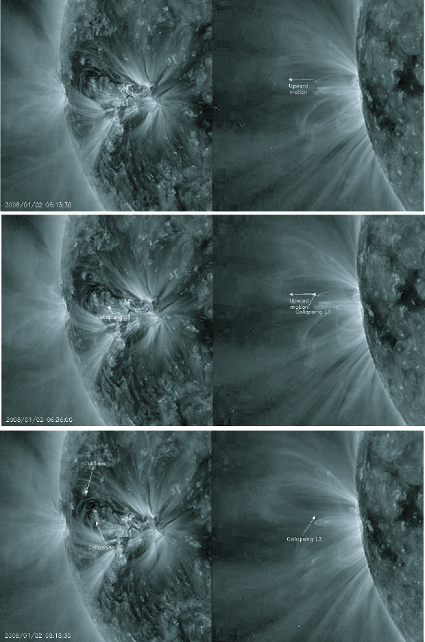
Figure 2.: Snapshots of the eruption as seen in simultaneous images from SECCHI/EUVI-A (right) and EUVI-B (left). The frames are taken from the online movie and the labeled features are discussed in Sections sec:height - sec:collapsing. The times correspond to the EUVI-A observation time. fig:detail

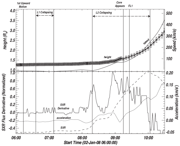
Figure 3.: The development of the eruption as seen through height-time and velocity-time diagrams (top panel) and the Soft X-ray light curve and its derivative (bottom panel). The heights correspond to the top of the CME structure and the speed is derived using a smoothing procedure (Section 2.2). Key events, such as collapsing loops, are also marked on the figure and are discussed in Sections 2.3 and 2.4. fig:CME˙height

The last height measurement was taken in COR1-A at 10:50:18 UT but we show results only until 10:30 UT. At that point the CME has reached a height of $3R_{\odot}$ with velocity of $420$ km s^-1. Both our speed and acceleration results are consistent with the Zhao10 results which were based on ht measurements after 10:00:00 UT and on a different technique.

In the bottom panel of Figure fig:CME_height, we compare the CME acceleration to the 1-min GOES SXR light curve (1-8Å channel) and its time derivative which is considered a proxy to energy release episodes. Both SXR curves are normalized to their respective peaks.

First, we see that the CME acceleration profile follows closely the SXR rise as seen before [Zhang et al. (2004), Temmer et al. (2008), Temmer et al. (2010)], albeit with some time delay. This delay is consistent with the gradual character of this CME. Generally speaking, impulsive CMEs tend to have acceleration profiles leading the SXR flux profile [Patsourakos, Vourlidas, and Stenborg (2010)] since it takes some time to heat the chromosphere and to fill in the coronal loops with the hot plasma. In our case, the CME acceleration peaks sharply after at about 10:23 UT when the flux rope core and the post-CME flaring arcades appear. We return to this point in Section sec:flux-rope.

Second, the impulsive phase of flare is a bit unusual because the rise of the SXR flux is marked by two interim inflections (one at $\sim$8:25-8:50 and the second at 9:20 UT) before the SXR peak at 10:00 UT. Remarkably, the CME acceleration profile changes at almost the same times. We can discern inflection points at approximately 8:30, 8:55, 9:10, 9:20, 9:55, and 10:25 UT in the bottom panel of Figure fig:CME_height. These points bracket intensity changes in the SXR light curve and coincide with peaks in the SXR derivative (and hence energy release episodes). The correlations are positive (acceleration) with the exception of the SXR derivative peak at 9:10 UT which occurs during a decelerating phase of the CME. The time offsets between the SXR and CME acceleration peaks are within 5 min of each other. There is even indication for an earlier acceleration jump associated with a small step in the SXR flux at around 7:00 UT. Since flaring and hence changes in the SXR profile result from energy release in the low corona, it is tempting to interpret the changes in the CME acceleration profile as a result of the same energy release. For example, the CME speed increases from about 5 km s^-1 to almost 80 km s^-1 during the first flaring episode, between 8:20 and 9:00 UT. To investigate whether the correspondence between the SXR and CME acceleration profiles is based on a causal relationship we look into the various phases of the event in detail in the following.

2.3 Collapsing Loops

sec:collapsing

The observation of the two collapsing loop systems, L1 and L2, represents a unique aspect of this event and drew our attention to it. The first system, L1, appears to be a single loop which stands out because it is projected against an area of reduced 171Å emission, possibly a cavity, as viewed from EUVI-A. The loop appears to collapse starting at around 6:36 UT and disappears at 7:21 UT. The loops do not appear to simply contract as has been seen in other occasions (see 2011SSRv..158….5H and references therein) but it rather seems to incline toward the cavity. At the same time, the cavity is slowly rising and expanding. This behavior, especially the disappearance of the loop, is seen for the first time and is suggestive of a magnetic relationship between the loop and the cavity. But before we discuss this further, we have to understand the 3D topology of the loop.

The loop is quite tall (0.15 R_⊙ or $1.04\times 10^{5}$ km). However, it is very hard to discern from the EUVI-B perspective because it is narrow (small footpoint distance) and is oriented toward EUVI-B (Figure fig:detail, middle panels). Nevertheless, its 3-dimensional (3D) orientation can be established because it becomes visible in EUVI-B once it starts collapsing. We use standard SECCHI software (the scc_measure routine) to derive its 3D parameters as a function of time for the period 6:36-7:08 UT. Briefly, the algorithm requires the user to select a point in the loop in one view. This selection corresponds to a line (the epipolar line) in the other view. The successful triangulation is achieved by identifying the location where the epipolar line intersects the projection of the original point in the loop. In our case, the obvious candidate is the bright loop-top in EUVI-A. Unfortunately it does not have a clearly identifiable counterpart in EUVI-B because we view the loop-top face-on. After careful examination of the movies, we decided to use a relatively bright edge in EUVI-B as the starting point because it was easier to find the intersection of the epipolar line with the loop in the EUVI-A images. The intersection was located a few pixels below the bright loop apex along the loop leg farthest from the EUVI-A observer. Here, we are primarily interested in the temporal behavior of the loop height. The ht measurements are shown in the Figure fig:collapsing-loops-ht. There is an obvious downward trend despite some scatter in the measurements around 7 UT. The scatter arises from inaccurate identification of the same part of the structure in the two images. We repeated the measurements three times but we were not able to improve the scatter in time. Although the scatter in the three measurements (at the same time) was very small, we decided to adopt a conservative error estimate equal to the standard deviation of all measurements in order to account for the scatter in time. Given the scatter, we fit the ht data points with a first order polynomial, assuming therefore, a constant speed. We obtained a speed of $3$ km s^-1.

Figure 4.: Height-time measurements of the two sets of collapsing loops observed during this CME event. The heights are true radial distances obtained via triangulation of the structures in the EUVI-A and -B 171Å images. The solid lines represent linear fits to the ht points and result in speeds of 3 km s^-1 and 2 km s^-1 for the L1 and L2 systems, respectively.fig:collapsing-loops-ht

Just an hour later, at 8:18 UT, a larger loop system (L2) begins to collapse following an almost identical path to L1 (Figure fig:infalling-loops). The L2 system is located just a few pixels southeast of L1 and reaches almost the same height, 0.15 R_⊙. L2 is more discernible in the EUVI-B images but it could easily be overlooked if it was not for the EUVI-A observations. This is a very important point and explains the lack of such observations in the past. How many times have we missed such inclining, collapsing loops in the past because we had only one viewpoint available? Thanks to the two EUVI views, we can derive the 3D orientation of L2 as we did for L1. The resulting ht points in Figure fig:collapsing-loops-ht show a rather sharp drop in the first 15 mins followed by a gradual contraction. We chose to fit again a first order polynomial to describe the long-term evolution of the loop apex. In this case, we derived a slight slower speed of $2$ km s^-1. The L2 system collapses toward the bottom of the erupting structure and the cavity is clearly rising while the loop system is collapsing. The loops disappear similarly to L1, at a height of 0.12 R_⊙. We note that the CME clearly took off while the L2 system was still collapsing and that the disappearance of the L2 loops coincides with the flare peak. It is also worth noting (Figure fig:detail) that the first set of bright flaring loops (in 171Å) appears at the location of the L2 footpoints.

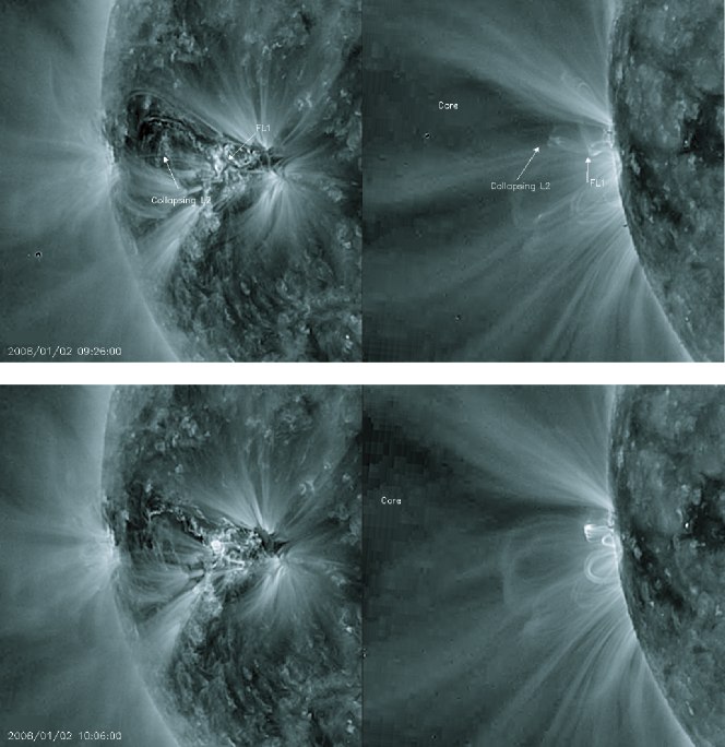
Figure 5.: The collapsing loops toward the expanding CME cavity as seen from EUVI-A (top right) and EUVI-B (top left). The arrows point to the direction of the collapse. A flaring loop system with peculiar connectivity is also marked (FL1). The bottom panels show snapshots at the time of the disappearance of the L2 system and the appearance of bright flaring loops at their footpoints.fig:infalling-loops

The coincidence of the collapsing loops to the rise and growth of the erupting structure is very suggestive of a magnetic connection between the two and is expected according to the standard CME models. Specifically, the models show that as the flux rope rises and a current sheet forms behind it, the resulting reconnection attracts nearby magnetic lines. The result is the creation of a void which field lines further afield would rush to fill. The void, and subsequent inflow, would occur across the erupting channel. Because most models are essentially two-dimensional, the reconnection is symmetric and proceeds from the center of the neutral line (or filament channel) outwards and across the channel. In this situation, the inflows are depicted on either side of the post-CME current sheet (e.g., 2004ApJ…602..422L). However, this does not have to be, and most likely it is not the situation with the actual observations. Erupting prominences (a usual proxy for the CME core) are often seen rising asymmetrically and the majority of H$\alpha$ ribbons brighten progressively both across and along the channel. If the eruption were to start at one end of the filament channel then the ribbons would move from that end of the channel to the opposite instead from starting at the middle and propagate outwards along the channel as the symmetric picture would suggest [Li and Zhang (2009)]. In that case, the void would form on end of the channel and any likely inflows would occur there. Such an asymmetric eruption was discussed by Patsourakos_Vourlidas_Kliem_2010. Therefore, we expect the following: (i) inflows toward and behind the erupting structure, (ii) the inflows would occur where the flux rope rises first, and (iii) the inflows and flux rope growth would be correlated. The analysis of the collapsing loops meets all three of these expectations and hence we claim that they constitute the first direct evidence of the process of flux rope formation (or growth) though the incorporation of neighboring flux systems into the erupting structure.

2.4 The Detection of the Hot Flux Rope Core

sec:flux-rope

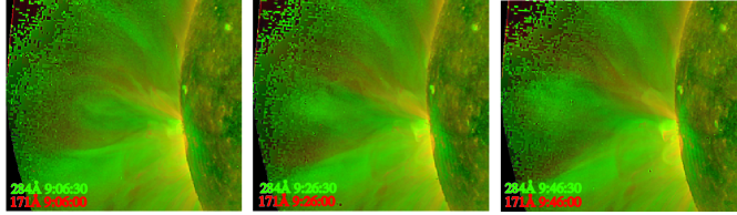
Figure 6.: Overlays of quasi-simultaneous EUVI-A observations at 284Å (green) and 171Å (red) during the appearance of the CME core. The degree of color dominance (green or red) at a given location can be used as a proxy for the temperature of the material at that location. For example, the CME core appears fully green at 9:26 UT which implies that most of the core material is emitting at 284Å or about 1.8 MK, at that time.fig:fluxrope

The CME has a clear 3-part structure in the COR1 and COR2 observations [Zhao et al. (2010)] and both the front and following cavity are easily discernible in the 171Å observations. The counterpart for the core is not easy to identify until 9:15 UT when a rather diffuse blob-like structure appears in the 195Å images. No erupting prominence is detected in the 304Å observations. The core is clearly visible in the 284Å image taken at 9:26:30 UT but it is very hard to detect in the almost simultaneous 171Å image at 9:26 UT (Figure fig:fluxrope). The dominant contribution in the 284Å bandpass comes from the FeXV line which forms at around 1.8 MK. Therefore, the lack of 171Å emission and the bright 284Å emission suggest that the majority of the core plasma comes from hot temperatures. This is exactly what the models predict and recent Solar Dynamics Observatory (SDO) observations show [Cheng et al. (2011)]. Therefore, we conclude that the CME core in our event is hot and comes at the tail end of the cavity within the erupting structure. Once the core is identified in the 284Å and 194Å images, it is relatively straightforward to follow in the 171Å as well although it remains quite faint (see online movie).

2.5 Flows along the Filament Channel

Throughout the event, one can observe flows along the filament channel (FC). They become more obvious along a bend of the FC at its eastern end. The filament itself is observed as a collection of dark threads in the 171Å channel due to the absorption from the cool material. It is anchored in the AR on its western end and in the quiet sun at its eastern end. The flows seem to evolve in two phases. In the first one, which lasts until 8:28 UT, the flows are brighter. In the second phase, which lasts until 10:06 UT, the flowing material acquires a blob-like character. Some of those blobs are depicted in Figure fig:siphon. The symbols in this figure (cross, box, circle) indicate the position the blobs we identified and measured at different time frames. In Figure fig:blobs, the area of interest has been rotated to make the blob movement more obvious. The position of each blob in this sequence of images is connected with a line.

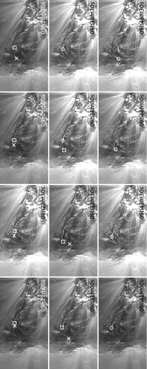
Figure 7.: Flows along the erupting filament channel. The symbols indicate a particular blob tracked at different times in each of these EUVI-B 171Å images. fig:siphon

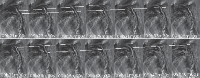
Figure 8.: Demonstration of our tracking of the blobs in the EUVI-B images. The area was rotated to make easier the display of lines connecting the blobs. In the top panels, the upper line traces the blob marked with an X in Figure fig:siphon, and the lower line traces the blob marked with a box. In the bottom panels, the first two frames are repeats from the last two frames of the top panel. The upper line is the continuation of the trace for the blob marked with the box symbol, and the lower line traces the blob marked with the circle. fig:blobs

After tracing the blobs, we measured their velocities. When the size of blobs was small (e.g. at 09:23:00 UT), their position was assumed to be their coordinates in the image. When the blobs became more extended (e.g. at 09:38:30 UT), we took the middle point as their average position, and their length was taken as the error uncertainty.

Because the blobs were located very low in the corona, they were not visible from EUVI-A. Because we know the angular distance of EUVI-A and the location of the flows from EUVI-B, we can derive an upper limit for the height of the channel of 0.015 R_⊙ or $10.5\times 10^{4}$ km. Since they move parallel to the surface and over a limited spatial extension, there was no need to correct for spherical geometry. The effect is less than 4% for the full $30^{\circ}$ length of the filament which we did not use in our measurements. However, the projection effect due to the proximity of the channel to the limb needs to be taken into account. The flows are measured at about $65^{\circ}$ east longitude so the correction factor is $\sim 1/cos(65^{\circ})\sim 2.36$. The average deprojected velocities of the blobs are given in Table tab:siphon. Each blob is named after the symbol we used to mark them in Figure fig:siphon.

The relation of the flows to the eruption is not immediately clear. First, they appear to correspond to material flowing out of the AR into the quiet sun because they propagate only in one direction, from the center of the AR toward the quiet sun. Such behavior has been very common since the beginning of EUVI observations and is always related to AR filaments that extend into the quiet sun. Examples can be seen in the eruptions of 1, 16, and 19 May 2009, 5 and 9 April 2008, 14 and 18 August 2010. The event on 3 April 2010 has been analyzed in the detail by 2011ApJ…727L..10S who connect such flows to off-loading of cool plasma that may contributed to the subsequent CME eruption. Second, the nature of the blobs changes at around 8:28 UT from thick elongated flows to smaller blob-like features suggesting that the amount of the flowing material has been reduced or the plasma has cooled down. It is interesting to note that the CME underwent its first acceleration jump during that time. This apparent correlation seems to support the 2011ApJ…727L..10S interpretation of the flows as off-loading material and suggests that gravity may affect the early acceleration profile of CMEs.

Table 2.: Average velocities for each of the three blobs. The names correspond to the symbols used to mark the blobs in Figure fig:siphon.

Blob	Velocity $(km\,s^{-1})$	Error
X	125	5.3
Box	116	4.9
Circle	130	5.4

tab:siphon

There is an alternative explanation, however. The flows apparently trace closed field lines along the filament. The movement of the blobs is directed away from the site of the emerging fluxrope where energy input is taking place leading to higher plasma pressures in its vicinity. Therefore, the observed flows could be siphon flow imposed by a pressure difference between the two footpoints of the filament [Cargill and Priest (1980), Cargill and Priest (1982)].

3 Discussion and Conclusions

We investigate in detail the initiation and formation of a CME on January 2, 2008 using two-viewpoint EUV observations in the lower corona. The images are obtained in the 171Å (150 sec cadence) and 284Å (20 min cadence) channels of the EUVI instruments aboard the STEREO mission. The event evolves slowly for several hours but it then quickly accelerates around the time of the accompanying SXR flare. This allows us to study in detail both its evolution toward the eruption, the subsequent formation of a CME, and its connection to the flare energy release profile. Our main results can be summarized as follows:

• The acceleration profile of the CME is quite variable with peaks and valleys. The acceleration changes are similar, in time of appearance and duration, with corresponding changes in the GOES SXR light curve.

• The CME acceleration peaks at 10:30 UT which is 30 mins after the peak of the SXR flare.

• The upward motions of the (eventually) erupting structure started at 6:13 UT, about 1 hour before a small SXR flux increase and 2 hours before a significant increase of SXR flux occurred (Figure fig:CME_height).

• We detect, for the first time, two sets of collapsing loops. The two viewpoint EUVI observations allow us to measure their 3D evolution. They shrink very little (compared to past observations of shrinking loops) so most of their collapse is due to their inclining toward the erupting channel, beneath the rising cavity. They appear in all EUVI channels and they disappear in all of them at a height of 0.12 R_⊙. The post-CME arcades appear after the disappearance of the collapsing loops and at the same location. The CME cavity is clearly growing while the second loop system (L2) is collapsing. These observations lead us to conclude that the two loop systems are likely drawn behind the expanding magnetic cavity surrounding the CME core. This appears to be the first detection of this process predicted by CME initiation models.

• We detect the core of the CME mostly in the hot EUVI channel at 284Å (1.8 MK) and the 195Å channel. This observation provides further support that the CME cavity contains hot plasma as recent AIA observations have shown [Cheng et al. (2011)].

• We detect significant and long duration ($\sim 3$ hours) plasma flows along the filament channel before its eruption. Their nature changes abruptly at around 8:30 UT coincident with a sudden change in the rising speed of the cavity. This coincidence suggests that mass unloading is perhaps playing a role in the early CME kinematics.

• The direction of the flows, from the western to the eastern part of the active region, is also in agreement with the temporal evolution of the flaring ribbons and post-eruptive flaring arcades, and the direction of the collapsing loops. Clearly, the eruption starts at the center of the active region and propagates to the east along the filament channel and toward the quiet sun footpoints of that channel.

• Despite the large number of novel observations and detailed measurements we cannot tell with certainty whether the erupted flux rope was pre-existing or was formed during the eruption. However, we are fairly certain that additional flux was introduced in the erupting flux rope during its ascent. This is the second event we reach this conclusion [Patsourakos, Vourlidas, and Kliem (2010)] and is the expected outcome of several models [Lin, Raymond, and van Ballegooijen (2004), Forbes et al. (2006), Chen (2011)]. It is, therefore, important to take this effect into account in the estimation of magnetic flux entrained in CMEs.

All these observations confirm corresponding expectations of the standard flare-CME models and suggest that such models are likely reliable representations of the eruption process in the corona. Our analysis demonstrates the power of two-viewpoint observations of the low corona and the importance of extended fields of view for EUV instruments so that the acceleration profile of the CME and the relationships among the various erupting structures can be measured consistently.

Acknowledgements

We thank the referee for the very useful comments and G. Stenborg for providing the wavelet-enhanced EUVI images and S. Patsourakos for fruitful discussions. The work of AV is supported by NASA contract S-136361-Y to the Naval Research Laboratory. The SECCHI data are produced by an international consortium of the NRL, LMSAL and NASA GSFC (USA), RAL and Univ. Bham (UK), MPS (Germany), CSL (Belgium), IOTA and IAS (France).

References

- Cargill and Priest (1980) Cargill, P.J., Priest, E.R.: 1980, Sol. Phys. 65, 251. doi:10.1007/BF00152793.
- Cargill and Priest (1982) Cargill, P.J., Priest, E.R.: 1982, Geophysical and Astrophysical Fluid Dynamics 20, 227. doi:10.1080/03091928208213654.
- Chen (2011) Chen, P.F.: 2011, Living Reviews in Solar Physics 8, 1.
- Cheng et al. (2011) Cheng, X., Zhang, J., Liu, Y., Ding, M.D.: 2011, ApJ 732, L25. doi:10.1088/2041-8205/732/2/L25.
- Forbes et al. (2006) Forbes, T.G., Linker, J.A., Chen, J., Cid, C., Kóta, J., Lee, M.A., Mann, G., Mikić, Z., Potgieter, M.S., Schmidt, J.M., Siscoe, G.L., Vainio, R., Antiochos, S.K., Riley, P.: 2006, Space Sci. Rev. 123, 251. doi:10.1007/s11214-006-9019-8.
- Howard et al. (2008) Howard, R.A., Moses, J.D., Vourlidas, A., Newmark, J.S., Socker, D.G., Plunkett, S.P., Korendyke, C.M., Cook, J.W., Hurley, A., Davila, J.M., Thompson, W.T., St Cyr, O.C., Mentzell, E., Mehalick, K., Lemen, J.R., Wuelser, J.P., Duncan, D.W., Tarbell, T.D., Wolfson, C.J., Moore, A., Harrison, R.A., Waltham, N.R., Lang, J., Davis, C.J., Eyles, C.J., Mapson-Menard, H., Simnett, G.M., Halain, J.P., Defise, J.M., Mazy, E., Rochus, P., Mercier, R., Ravet, M.F., Delmotte, F., Auchere, F., Delaboudiniere, J.P., Bothmer, V., Deutsch, W., Wang, D., Rich, N., Cooper, S., Stephens, V., Maahs, G., Baugh, R., McMullin, D., Carter, T.: 2008, Space Science Reviews 136, 67. doi:10.1007/s11214-008-9341-4.
- Hudson (2011) Hudson, H.S.: 2011, Space Sci. Rev. 158, 5. doi:10.1007/s11214-010-9721-4.
- Kaiser et al. (2008) Kaiser, M.L., Kucera, T.A., Davila, J.M., St. Cyr, O.C., Guhathakurta, M., Christian, E.: 2008, Space Science Reviews 136, 5. doi:10.1007/s11214-007-9277-0.
- Klimchuk (2001) Klimchuk, J.A.: 2001, Space Weather (Geophysical Monograph 125), ed. P. Song, H. Singer, G. Siscoe (Washington: Am. Geophys. Un.), 143 (2001) 125, 143.
- Li and Zhang (2009) Li, L., Zhang, J.: 2009, ApJ 690, 347. doi:10.1088/0004-637X/690/1/347.
- Lin, Raymond, and van Ballegooijen (2004) Lin, J., Raymond, J.C., van Ballegooijen, A.A.: 2004, ApJ 602, 422. doi:10.1086/380900.
- Patsourakos, Vourlidas, and Kliem (2010) Patsourakos, S., Vourlidas, A., Kliem, B.: 2010, A&A 522, A100. doi:10.1051/0004-6361/200913599.
- Patsourakos, Vourlidas, and Stenborg (2010) Patsourakos, S., Vourlidas, A., Stenborg, G.: 2010, ApJ 724, L188. doi:10.1088/2041-8205/724/2/L188.
- Reeves (2006) Reeves, K.K.: 2006, ApJ 644, 592. doi:10.1086/503352.
- Seaton et al. (2011) Seaton, D.B., Mierla, M., Berghmans, D., Zhukov, A.N., Dolla, L.: 2011, ApJ 727, L10. doi:10.1088/2041-8205/727/1/L10.
- Stenborg, Vourlidas, and Howard (2008) Stenborg, G., Vourlidas, A., Howard, R.A.: 2008, ApJ 674, 1201. doi:10.1086/525556.
- Švestka and Cliver (1992) Švestka, Z., Cliver, E.W.: 1992, In: Z. Švestka, B. V. Jackson, & M. E. Machado (ed.) IAU Colloq. 133: Eruptive Solar Flares, Lecture Notes in Physics, Berlin Springer Verlag 399, 1. doi:10.1007/3-540-55246-4_70.
- Temmer et al. (2008) Temmer, M., Veronig, A.M., Vršnak, B., Rybák, J., Gömöry, P., Stoiser, S., Maričić, D.: 2008, ApJ 673, L95. doi:10.1086/527414.
- Temmer et al. (2010) Temmer, M., Veronig, A.M., Kontar, E.P., Krucker, S., Vršnak, B.: 2010, ApJ 712, 1410. doi:10.1088/0004-637X/712/2/1410.
- Zhang et al. (2004) Zhang, J., Dere, K.P., Howard, R.A., Vourlidas, A.: 2004, ApJ 604, 420. doi:10.1086/381725.
- Zhao et al. (2010) Zhao, X.H., Feng, X.S., Xiang, C.Q., Liu, Y., Li, Z., Zhang, Y., Wu, S.T.: 2010, ApJ 714, 1133. doi:10.1088/0004-637X/714/2/1133.