Empirical Bayes estimation of posterior probabilities of enrichment

Abstract

Background: To interpret differentially expressed genes or other discovered features, researchers conduct hypothesis tests to determine which biological categories such as those of the Gene Ontology (GO) are enriched in the sense of having differential representation among the discovered features. Multiple comparison procedures (MCPs) are commonly used to prevent excessive false positive rates. Traditional MCPs, e.g., the Bonferroni correction, go to the opposite extreme of strictly controlling a family-wise error rate, resulting in excessive false negative rates. Researchers generally prefer the more balanced approach of instead controlling the false discovery rate (FDR). Methods of FDR control assign q-values to biological categories, but q-values are too low to reliably estimate a probability that the biological category has equivalent representation among the preselected features. Thus, we study application of better estimators of that probability, which is technically known as the local false discovery rate (LFDR).

Results: We identified three promising estimators of the LFDR for detecting differential representation: a semiparametric estimator (SPE), a normalized maximum likelihood estimator (NMLE), and a maximum likelihood estimator (MLE). We found that the MLE performs at least as well as the SPE for on the order of 100 of GO categories even when the ideal number of components in its underlying mixture model is unknown. However, the MLE is unreliable when the number of GO categories is small compared to the number of PMM components. Thus, if the number of categories is on the order of 10, the SPE is a more reliable LFDR estimator. The NMLE depends not only on the data but also on a specified value of the prior probability of differential representation. It is therefore an appropriate LFDR estimator only when the number of GO categories is too small for application of the other methods.

Conclusions: For enrichment detection, we recommend estimating the LFDR by the MLE given at least a medium number ($\sim$100) of GO categories, by the SPE given a small number of GO categories ($\sim$10), and by the NMLE given a very small number ($\sim$1) of GO categories.

¹Ottawa Institute of Systems Biology, Department of Biochemistry, Microbiology, and Immunology, University of Ottawa, 451 Smyth Road, Ottawa, Ontario, Canada, K1H 8M5

²School of Foundation, Shenyang Pharmaceutical University, No. 103 Wenhua Road, Shenyang, Liaoning, 110016, China

E-mail: zyang009@uottawa.ca; zuojing1006@hotmail.com; dbickel@uottawa.ca

^∗Corresponding author

Keywords: empirical Bayes, gene enrichment, gene expression, Gene Ontology, local false discovery rate, minimum description length, multiple comparison procedure, normalized maximum likelihood, simultaneous inference

Introduction

The development of microarray techniques and high-throughput genomic, proteomic, and bioinformatics scanning approaches (such as microarray gene expression profiling, mass spectrometry, and ChIP-on-chip) has enabled researchers simultaneously to study tens of thousands of biological features (e.g., genes, proteins, single-nucleotide polymorphisms [SNPs], etc.), and to identify a set of features for further investigation. However, there remains the challenge of interpreting these features biologically. For a given set of features, the determination of whether some biological information terms are differentially represented (i.e., overrepresented or underrepresented), compared to the reference feature set, is termed the feature enrichment problem. The biological information term may be, for instance, a Gene Ontology (GO) category [1] or a pathway in the Kyoto Encyclopedia of Genes and Genomes (KEGG) [20].

This problem has been addressed using a number of high-throughput enrichment tools, including DAVID [10], MAPPFinder [11], Onto-Express [21], and GoMiner [31]. Huang et al. [18] reviewed $68$ distinct feature enrichment analysis tools. These authors further classified feature enrichment analysis tools into $3$ categories: singular enrichment analysis (SEA), gene set enrichment analysis (GSEA) and modular enrichment analysis (MEA). Here, we investigate the SEA problem using gene expression as a concrete example. More precisely, we consider whether some specific biological categories are differentially represented among the preselected genes with respect to the reference genes. We call this problem the gene enrichment problem.

Existing enrichment tools mainly address the gene enrichment problem using a p-value obtained from an exact or approximate statistical test (e.g., Fisher’s exact test, or the hypergeometric test, binomial test, $\chi^{2}$ test, etc.). For each GO term or other biological category, the null hypothesis tested and its alternative hypothesis are these:

$$\begin{array}[]{c}H_{0}:\text{ the GO category is equivalently represented among the preselected genes}\text{ }\\ H_{1}:\text{ the GO category is differentially represented among the preselected genes}\end{array}$$ (1)

The general process begins as follows:

• For each GO category, construct Table 1 based on the preselected genes (e.g., differentially expressed (DE) genes) and reference genes (e.g., all genes measured in a microarray experiment).

• Compute the p-value for each GO category using a statistical test that can detect enrichment in the sense of differential representation among the preselected genes.

Table 1: The number of differentially expressed (DE) and equivalently expressed (EE) genes in a GO category. Here, $x_{i}$ ($i=1,2$) is the number of DE ($i=1$) or EE genes ($i=2$) in the GO category; $n$ is the total number of DE genes; $N$ is the total number of reference genes.

	DE genes	EE gene	Total
In GO category	$x_{1}$	$x_{2}$	$x_{1}+x_{2}$
Not in GO category	$n-x_{1}$	$N-n-x_{2}$	$N-x_{1}-x_{2}$
Total	$n$	$N-n$	$N$

Multiple comparison procedures (MCPs) are then applied to the resulting p-values to prevent excessive false-positive rates. The false discovery rate (FDR) [3] is frequently used to control the expected proportion of incorrectly rejected null hypotheses in gene enrichment studies [22, 25, 29] because it has lower false-negative rates than the Bonferroni correction and other methods of controlling the family-wise error rate. Methods of FDR control assign q-values [28] to biological categories, but q-values are too low to reliably estimate the probability that the biological category has equivalent representation among the preselected features. Thus, we study application of better estimators of that probability, which is technically known as the local false discovery rate (LFDR). Hong et al. [17] used an LFDR estimator to solve a GSEA problem and pointed out that this was less biased than the q-value for estimating the LFDR, the posterior probability that the null hypothesis is true.

Efron [12, 13] devised reliable LFDR estimators for a range of applications in microarray gene expression analysis and other problems of large-scale inference. However, whereas microarray gene expression analysis takes into account tens of thousands of genes, the gene enrichment problem typically concerns a much smaller number of GO categories. While those methods are appropriate for microarray-scale inference, they are less reliable for enrichment-scale inference Bickel [4, 9]. Thus, we will specifically adapt three types of LFDR estimators that are appropriate for smaller-scale inference to address the SEA problem. Here we will focus on genes and GO categories. Nevertheless, the estimators used can be broadly applied to other features (e.g., proteins, SNPs) and biological terms (e.g., those featuring metabolic pathways).

The sections of this paper are arranged as follows. We will first introduce some preliminary concepts in the gene enrichment problem. Next, $3$ LFDR estimators will be described. After that, we will compare the LFDR estimators using breast cancer data and simulation data. Finally, we will draw conclusions and make recommendations on the basis of our results.

Preliminary concepts

The gene enrichment problem described in the Introduction is stated here more formally for application of LFDR methods of the next section.

Likelihood functions

Consider Table 1. Let $X_{1}$ and $X_{2}$ respectively denote the random numbers of DE and EE genes in a GO category. The resulting categories follow the binomial distribution, i.e.,$X_{1}\sim\text{Binomial}(n,\Pi_{1})$ and $X_{2}\sim\text{Binomial}(N-n,\Pi_{2})$, where $\Pi_{1}$ is the proportion of DE genes in the GO category and $\Pi_{2}$ is the proportion of EE genes in the GO category. Under the assumption that $X_{1}$ and $X_{2}$ are independent, the unconditional likelihood is

$$L(\Pi_{1},\Pi_{2};x_{1},x_{2},n,N)$$ (2)

$$=\text{Pr}(X_{1}=x_{1},X_{2}=x_{2};\Pi_{1},\Pi_{2},n,N)$$

$$=\binom{n}{x_{1}}\binom{N-n}{x_{2}}\Pi_{1}^{x_{1}}(1-\Pi_{1})^{n-x_{1}}\Pi_{2}^{x_{2}}(1-\Pi_{2})^{N-n-x_{2}}$$

where $0\leq x_{1}\leq n$, $0\leq x_{2}\leq N-n$ and $0\leq\Pi_{i}\leq 1$, $i=1,2$.

If we define

$$\lambda=\ln[\Pi_{2}/(1-\Pi_{2})]$$ (3)

and

$$\theta=\ln[\Pi_{1}/(1-\Pi_{1})]-\lambda$$ (4)

then $\theta$ is the parameter of interest, representing the log odds ratio of the GO category, and $\lambda$ is a nuisance parameter. Under the new parametrization, the unconditional likelihood function (2) is

$$L(\theta,\lambda;x_{1},x_{2},n,N)=\frac{\binom{n}{x_{1}}\binom{N-n}{x_{2}}\times e^{x_{1}(\theta+\lambda)}e^{x_{2}\lambda}}{(1+e^{\theta+\lambda})^{n_{1}}(1+e^{\lambda})^{n_{2}}}$$ (5)

where $0\leq x_{1}\leq n$ and $0\leq x_{2}\leq N-n$.

In equation (5), we take the interest parameter $\theta$ and also the nuisance parameter $\lambda$ into consideration. Consider statistics $T$ and $S$, functions of $X_{1}$ and $X_{2}$, such that $T(X_{1},X_{2})=X_{1}$ and $S(X_{1},X_{2})=X_{1}+X_{2}$. Thus, $T$ represents the number of DE genes in a GO category, and $S$ represents the number of total genes in a GO category. Let $t$ and $s$ be the observed values of statistic $T$ and $S$. The probability mass function of $T(x_{1},x_{2})=t$ evaluated at $S(x_{1},x_{2})=x_{1}+x_{2}=s$, say $\text{Pr}(T=t|S=s;\theta,\lambda,N,n)$, does not depend on the nuisance parameter $\lambda$ [4]. See also Example $8.47$ of Severini [27]. Thus, we derive the conditional probability mass function

$$f_{\theta}(t|s)=\text{Pr}(T=t|S=s;\theta,n,N)=\frac{\binom{n}{t}\binom{N-n}{v-t}e^{t\theta}}{\sum_{j=\max(0,s+n-N)}^{\min(s,n)}\binom{n}{j}\binom{N-n}{s-j}e^{j\theta}}$$ (6)

understood as a function of $t$.

By eliminating the nuisance parameter $\lambda$, we can reduce the original data $x_{1}$ and $x_{2}$ by considering the statistic $T=t$. However, the use of the conditional probability mass function requires some justification because of concerns about losing information during the conditioning process. Unfortunately, in the presence of the nuisance parameter, the statistic $S(X_{1},X_{2})=X_{1}+X_{2}$ is not an ancillary statistic for the parameter of interest. In other words, the probability mass function of the conditional variable $S(X_{1},X_{2})$ may contain some information about the parameter $\theta$ [27]. However, following the explanation of Barndorff-Nielsen and Cox [2, $\mathcal{x}2.5$], the expectation value of the statistic $S(X_{1},X_{2})$ equals the nuisance parameter. Hence, from the observation of $S(X_{1},X_{2})$ alone, the distribution of the statistic $S(X_{1},X_{2})$ contains little information about the parameter $\theta$ [2]. The statistic $S(X_{1},X_{2})$ satisfies the other $3$ conditions of an ancillary statistic defined by Barndorff-Nielsen and Cox [2]: parameters $\theta$ and $\lambda$ are variation independent; the statistic ($T(X_{1},X_{2}),S(X_{1},X_{2})$) is the minimal sufficient statistic; and the distribution of the statistic $T(X_{1},X_{2})$, given $S(X_{1},X_{2})=s$, is independent of parameter of interest, $\theta$, given the nuisance parameter $\lambda$. Therefore, the probability mass function of the statistic $S(X_{1},X_{2})$ contains little information about the value of the parameter $\theta$.

Hypotheses and false discovery rates

Considering GO category $i$, we denote the $T$, $S$, $t$, $s$ and $\theta$ used in equation (6) as $T_{i}$, $S_{i}$, $t_{i}$, $s_{i}$ and $\theta_{i}$. From Table 1, the hypothesis comparison (1) of GO category $i$ is equivalent to

$$\theta_{i}=0\text{ versus }\theta_{i}\neq 0$$ (7)

Let $\mathbf{S}=\left\langle S_{1},S_{2},\cdots,S_{m}\right\rangle$ and $\mathbf{s}=\left\langle s_{1},s_{2},\cdots,s_{m}\right\rangle$. Let $\text{BF}_{i}$ denote the Bayes factor of GO category $i$:

$$\text{BF}_{i}=\frac{\text{Pr}(T_{i}=t_{i}|\mathbf{S}=\mathbf{s},\theta_{i}\neq 0)}{\text{Pr}(T_{i}=t_{i}|\mathbf{S}=\mathbf{s},\theta_{i}=0)}$$ (8)

It is called the Bayes factor because it yields the posterior odds when multiplied by the prior odds. More precisely, the posterior odds of the alternative hypothesis corresponding to GO category $i$ is

$$\omega_{i}=\frac{\text{Pr}(\theta_{i}\neq 0|t_{i})}{\text{Pr}(\theta_{i}=0|t_{i})}=\text{BF}_{i}\times\frac{(1-\pi_{0})}{\pi_{0}}$$ (9)

where $\pi_{0}$ is the prior conditional probability that a GO category is equivalently represented among the preselected genes given $\mathbf{s}$, i.e., $\pi_{0}=\text{Pr}(\theta_{i}=0|\mathbf{S}=\mathbf{s})$. Thus, $(1-\pi_{0})/\pi_{0}$ is the prior odds of the alternative hypothesis of differential representation. According to Bayes’ theorem, the LFDR of GO category $i$ is

$$\text{LFDR}_{i}=\text{Pr}(\theta_{i}=0|t_{i})=\frac{1}{1+\omega_{i}},$$ (10)

where $\omega_{i}$ is defined in equation (9).

LFDR estimation methods

Semiparametric LFDR estimator

Let $\alpha$ denote any significance level chosen to be between 0 and 1. For all GO categories of interest, the FDR may be estimated by

$$\widehat{\text{FDR}}(\alpha) = \min\left(\frac{m\alpha}{\sum_{j=1}^{m}\mathbf{1}_{\{p_{j}\leq\alpha\}}},1\right)$$ (11)

where $m$ is the number of GO categories, $p_{j}$ is the p-value of GO category $j$, and $\mathbf{1}_{\{p_{j}\leq\alpha\}}$ is the indicator such that $\mathbf{1}_{\{p_{j}\leq\alpha\}}=1$ if $p_{j}\leq\alpha$ is true and $\mathbf{1}_{\{p_{j}\leq\alpha\}}=0$ otherwise. Thus, $\sum_{j=1}^{m}\mathbf{1}_{\{p_{j}\leq\alpha\}}$ represents the number of GO categories with discovered differential representation, and $m\alpha$ estimates the number of such discoveries that are false.

Let $r_{i}$ be the rank of the p-value of GO category $i$, e.g., $r_{i}=1$ if the p-value of GO category $i$ is the smallest among all p-values of $m$ GO categories. Based on a modification of equation (11), the semiparametric estimator (SPE) of LFDR of the GO category $i$ is

$$\widehat{\text{LFDR}}_{i}=\begin{cases}\min\left(\frac{mp_{2r_{i}}}{2r_{i}},1\right),&r_{i}\leq\frac{m}{2}\\ 1,&r_{i}>\frac{m}{2}\end{cases}$$ (12)

It is conservative in the sense that it tends to overestimate the LFDR [5].

Type II maximum likelihood estimator

Bickel [5] follows Good [15] in calling the maximization of likelihood over a hyperparameter Type II maximum likelihood to distinguish it from the usual Type I maximum likelihood, which pertains only to models that lack random parameters. Type II maximum likelihood has been applied to parametric mixture models for the analysis of microarray data [24, 23], proteomics data [9], and genetic association data [30]. In this section, we adapt the approach to the gene enrichment problem by using the conditional probability mass function defined above.

Let $\mathcal{G}(\mathbf{s})=\{g_{\theta}(\bullet|\mathbf{s});\theta\geq 0\}$ be a parametric family of probability mass functions with

$$g_{\theta}(\bullet|\mathbf{s}) = \frac{1}{2}\times\left[f_{\theta}(\bullet|\mathbf{s})+f_{-\theta}(\bullet|\mathbf{s})\right]$$ (13)

where $f_{\theta}(\bullet|\mathbf{s})$ is defined in equation (6). We define the $k$-component parametric mixture model ($k$-component PMM) as

$$g(\bullet|\mathbf{s};\theta_{0},\ldots,\theta_{k-1},\pi_{0},\ldots,\pi_{k-1}) = \sum_{i=0}^{k-1}\pi_{j}g_{\theta_{j}}(\bullet|\mathbf{s})$$ (14)

where $\theta_{0}=0$ and $\theta_{j}\neq\theta_{J}$, if $j\neq J$.

Let $\mathbf{T}=\left\langle T_{1},T_{2},\cdots,T_{m}\right\rangle$ and $\mathbf{t}=\left\langle t_{1},t_{2},\cdots,t_{m}\right\rangle$ be vectors of the $T_{i}$s and $t_{i}$s used in equation (8). Assuming $T_{i}$ is independent of $T_{j}$ and $S_{j}$ for any $i\neq j$, the joint probability mass function is

$$g(\mathbf{t}|\mathbf{s};\theta_{0},\ldots,\theta_{k-1},\pi_{0},\ldots,\pi_{k-1}) = \prod_{i=1}^{m}g(t_{i}|\mathbf{s};\theta_{0},\ldots,\theta_{k-1},\pi_{0},\ldots,\pi_{k-1})$$

$$= \prod_{i=1}^{m}g(t_{i}|s_{i};\theta_{0},\ldots,\theta_{k-1},\pi_{0},\ldots,\pi_{k-1})$$

where $s_{i}$ is the observed value of $S_{i}$ for GO category $i$, and $\mathbf{s}=\left\langle s_{1},s_{2},\cdots,s_{m}\right\rangle$.

Moreover, we assume that for given the number of genes in GO category $i$, $T_{i}$ $(i=1,\ldots,m)$, satisfies the $k$-component PMM shown in equation (14). In other words, we assume that the possible log odds ratios of GO category $i$ are the $\theta_{0},\theta_{1},\theta_{2},\ldots,\theta_{k-1}$ of equation (14) if the alternative hypothesis $H_{1}$ in the hypothesis comparison (7) is true.

Therefore, the log-likelihood function under the $k$-component PMM for all GO categories is

$$\log L(\theta_{0},\ldots,\theta_{k-1},\pi_{0},\ldots,\pi_{k-1}) = \log g(\mathbf{t}|\mathbf{s};\theta_{0},\ldots,\theta_{k-1},\pi_{0},\ldots,\pi_{k-1})$$ (16)

= $$\sum_{i=1}^{m}\left[\log\sum_{j=0}^{k-1}\pi_{j}g_{\theta_{j}}(t_{i}|s_{i})\right]$$

The LFDR of GO category $i$ is estimated by

$$\widehat{\text{LFDR}}_{i}^{\left(k\right)}=\frac{\widehat{\pi}_{0}g_{\theta_{0}}(t_{i}|s_{i})}{g(t_{i}|s_{i};\theta_{0},\widehat{\theta}_{1},\ldots,\widehat{\theta}_{k-1},\widehat{\pi}_{0},\ldots,\widehat{\pi}_{k-1})}$$ (17)

where $\widehat{\theta}_{1},\ldots,\widehat{\theta}_{k-1}$ and $\widehat{\pi}_{0},\ldots,\widehat{\pi}_{k-1}$ are maximum likelihood estimates of $\theta_{1},\ldots,\theta_{k-1}$ and $\pi_{0},\ldots,\pi_{k-1}$ in equation (16). We call $\widehat{\text{LFDR}}_{i}^{\left(k\right)}$ the $k$-component maximum likelihood estimator (MLE$k$).

LFDR estimator based on the normalized maximum likelihood

Combining equations (9)-(10), we obtain

$$\text{LFDR}_{i}=\left(1+\text{BF}_{i}\times\frac{(1-\pi_{0})}{\pi_{0}}\right)^{-1}$$ (18)

Therefore, given a guessed value of $\pi_{0}$, we may use an estimator of the Bayes factor to estimate the LFDR of a GO category.

We next develop such an estimator of the Bayes factor. For GO category $i$, let $\mathcal{E}_{i}$ stand for the set of all probability mass functions defined on $\left\{0,1,\dots,s_{i}\right\}$, the set of all possible values of $t_{i}$. Based on the hypothesis comparison (7), the set of log odds ratios, denoted as $\Theta$, is $\{0\}$ under the null hypothesis and is the set of all real values except $0$ under the alternative hypothesis. With the assumption that the random variable $T_{i}$ is independent of the random variable $S_{j}$ for any $i\neq j$, the regret of a predictive mass function $\bar{f}\in\mathcal{E}_{i}$ is a measure of how well it predicts the observed value $t_{i}\in\left\{0,1,\ldots,s_{i}\right\}$. The regret is defined as

$$\text{reg}(\bar{f},t_{i}|s_{i};\Theta)=\log\frac{f_{\hat{\theta}_{i}(t_{i}|s_{i})}(t_{i}|s_{i})}{\bar{f}(t_{i}|s_{i})}$$ (19)

where $\hat{\theta}_{i}(t_{i}|s_{i})$ is the Type I MLE with respect to the $\Theta$ under the observed values $t_{i}$ given $s_{i}$ [6, 16].

For all members of $\mathcal{E}_{i}$, the optimal predictive conditional probability mass function of GO category $i$, denoted as $f_{i}^{\dagger}$, minimizes the maximal regret in the sample space $\left\{0,1,\ldots,s_{i}\right\}$ in the sense that it satisfies

$$f_{i}^{\dagger}=\arg\min_{\bar{f}\in\mathcal{E}_{i}}\max_{t\in\left\{0,1,\ldots,s_{i}\right\}}\text{reg}(\bar{f},t|s_{i};\Theta)$$ (20)

It is well known [16] that the predictive probability mass function that satisfies equation (20) is

$$f_{i}^{\dagger}(t_{i}|s_{i};\Theta) = \frac{\max_{\theta\in\Theta}f_{\theta}(t_{i}|s_{i})}{\mathcal{K}_{i}^{\dagger}(\Theta)}$$ (21)

where $f_{\theta}(t_{i}|s_{i})$ is the conditional probability mass function defined in equation (6), and $\mathcal{K}_{i}^{\dagger}(\Theta)$ is the constant defined as

$$\mathcal{K}_{i}^{\dagger}(\Theta) = \max_{\theta\in\Theta}f_{\theta}(y|s_{i})$$

$$= \sum_{y=\max(0,s_{i}-n_{2})}^{\min(s_{i},n_{1})}\max_{\theta\in\Theta}f_{\theta}(y|s_{i})$$

$$= \sum_{y=\max(0,s_{i}-n_{2})}^{\min(s_{i},n_{1})}\frac{\binom{n_{1}}{y}\binom{n_{2}}{s_{i}-y}e^{y\hat{\theta}_{i}(y)}}{\sum_{j=\max(0,s_{i}-n_{2})}^{\min(s,n_{1})}\binom{n_{1}}{j}\binom{n_{2}}{s_{i}-j}e^{j\hat{\theta}_{i}(y)}}$$

where

$$\hat{\theta}_{i}(y)=\arg\max_{\theta\in\Theta}f_{\theta}(y|s_{i})$$ (23)

We call $f_{i}^{\dagger}(t_{i}|s_{i};\Theta)$ the normalized maximum likelihood (NML) associated with the hypothesis that $\theta_{i}\in\Theta$.

Thus, $\text{BF}_{i}$ is estimated by

$$\widehat{\text{BF}}_{i}^{\dagger}=\frac{f_{i}^{\dagger}(t_{i}|s_{i};{\theta:\theta\neq 0})}{f_{i}^{\dagger}(t_{i}|s_{i};{0})},$$ (24)

which we call the the NML ratio. Therefore, by combining equations (8) and (9), if we guess the prior probability $\pi_{0}$, the LFDR estimate of GO category $i$ in the hypothesis comparison (7) is

$$\widehat{\text{LFDR}}_{i}^{\dagger}=\left[1+\frac{1-\pi_{0}}{\pi_{0}}\times\widehat{\text{BF}}_{i}^{\dagger}\right]^{-1}$$ (25)

where $\widehat{\text{BF}}_{i}^{\dagger}$ is defined in equation (24). We call this LFDR estimator the normalized maximum likelihood estimator (NMLE).

To assess the performance of the NML ratio $\widehat{\text{BF}}_{i}^{\dagger}$, it will be compared to the following estimate of the Bayes factor. Equations (18) and (17) suggest

$$\widehat{\text{BF}}_{i}=\frac{1-\widehat{\text{LFDR}}_{i}^{\left(k\right)}}{\widehat{\text{LFDR}}_{i}^{\left(k\right)}}\times\frac{1-\widehat{\pi}_{0}}{\widehat{\pi}_{0}}$$ (26)

as an MLE-based estimator of $\text{BF}_{i}$.

Results

Breast cancer data analysis

The data set used here is from an experiment applying an estrogen treatment to cells of a human breast cancer cell line [26]. The data, which is available from the Bioconductor project, contains $8$ Affymetrix HG-U95Av2 CEL files from an estrogen receptor-positive breast cancer cell line. (For further information concerning the data and also the Bioconductor project, see Gentleman et al. [14].) For simplicity of terminology, we consider probes in the microarray experiment as genes, and use the $12,625$ genes expressed in the microarray experiment as a reference.

We selected as genes of interest those that were differentially expressed between two groups according to the following criterion. Using the LFDR as the probability that a gene is EE, we considered genes with LFDR estimates below $0.2$ as DE. In other words, we selected as DE genes those were differentially expressed with estimated posterior probability of at least $80\%$. We used the 2-sample t-test with equal variances to compute the p-value of each gene in the microarray. The LFDR of every gene is estimated using the theoretical null hypothesis method of Efron [12, 13]; empirical null hypotheses can lead to excessive bias due to deviations from normality [8]. When we compared gene expression data for the presence and absence of estrogen after $10$ hours of exposure, we obtained $74$ DE genes.

Defining unrelated pairs of GO categories as those that do not share any common ancestor, we selected for analysis all unrelated GO molecular function categories with at least $1$ DE gene, thereby obtaining a total of $82$ GO categories of interest. For each GO category, the p-value used in SPE to estimate LFDR is computed based on the 2-sided Fisher’s exact test. Figure 1 compares the SPE to the MLEs based on the $2$-component (MLE2) and $3$-component (MLE3) PMM. Figure 2 displays the probability mass of $\text{GO:}0005524$ under the null and alternative hypotheses of the hypothesis comparison (7). Figure 3 compares MLE-based estimates of the Bayes factor given by equation (26) to the NML ratios given by equation (26).

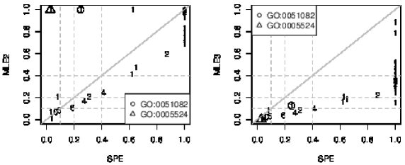
Figure 1: Comparison of the LFDR estimated by the SPE with the LFDR estimated by the MLE2 (left) and MLE3 (right). Each integer represents a number of GO categories. $\text{Intergers}>1$ indicate ties.

Figure 2: The conditional probability mass functions given the number of genes in $\text{GO:}0005524$ under a null hypothesis, and alternative hypotheses based on the $2$-component PMM (left) and $3$-component PMM (right). The grey dashed line is the number of DE genes in $\text{GO:}0005524$.

Figure 3: Comparison of the Bayes factor estimated by the NML ratio with that estimated by the MLE2 (left) and MLE3 (right). The integers are defined in Figure 1. The grey dashed lines mark commonly used thresholds for strong and overwhelming evidence [19, 7].

Simulation studies

The aim of the following simulation studies is to compare the LFDR estimation bias of SPE, MLE2, and MLE3. The NMLE is not taken into account because its performance depends not only on the data, but also on the specified prior probability $\pi_{0}$.

The simulation setting involves $10,000$ genes in a microarray with $200$ genes identified as DE and $100$ GO categories. We conducted a separate simulation study using each of these values of $\pi_{0}$: $50\%$, $60\%$, $70\%$, $80\%$, $90\%$, and $94\%$.

Since the PMM behind the MLE is optimal when the number of GO categories with overrepresentation (“enrichment”) is equal to the number with underrepresentation (“depletion”), we assessed the sensitivity of the MLE to that symmetry assumption by using strongly asymmetric log odds ratios as well as those that are symmetric. For each GO category, two configurations were used in this simulation to choose log odds ratios: the asymmetric configuration shown in equation (27) and the symmetric configuration shown in equation (28).

$$\theta_{i}^{\text{asymmetric}}=\begin{cases}\frac{5i}{100(1-\pi_{0})},&1\leq i\leq 100(1-\pi_{0})\\ 0,&100(1-\pi_{0})<i\leq 100\end{cases}$$ (27)

$$\theta_{i}^{\text{symmetric}}=\begin{cases}\frac{i}{10(1-\pi_{0})},&1\leq i\leq 50(1-\pi_{0})\\ 5-\frac{i}{10(1-\pi_{0})},&50(1-\pi_{0})<i\leq 100(1-\pi_{0})\\ 0,&100(1-\pi_{0})<i\leq 100\end{cases}$$ (28)

Considering the log odds ratios of all $100$ GO categories constructed by either the asymmetric or the symmetric configuration, we generated Table 1 for each GO category as follows:

• $x_{1}$ is generated from a binomial distribution with the parameter $\Pi_{1}$ used in equation (2); $\Pi_{1}$ is a real value randomly picked from $0$ to $1$ .

• $x_{2}$ is obtained from a binomial distribution with the parameter $\Pi_{2}=\left[\frac{(1-\Pi_{1})\times 2^{\theta_{i}}}{\Pi_{1}}+1\right]^{-1}$, obtained by solving equation (4).

The p-value of each GO category used in the SPE is obtained from 2-sided Fisher’s exact test. The $k$-component PMM ($k=2\text{ or }k=3$) used in the MLE is shown in equation (14) with $\pi_{j}=\left(1-\pi_{0}\right)/k\,\left[j=1,\dots,k\right]$ and $g_{\theta_{i}}(\bullet|s)=g_{\theta_{i}}(t_{i}|s_{i})$ defined in equation (13). For every log odd ratio sequence, we estimated the LFDR $20$ times using the SPE, MLE2, and MLE3. We compared the performances of the $3$ estimators by means of estimating the LFDR bias. The true LFDR is computed by equation (10), where

$$f_{0}(t_{i})=\frac{\binom{n}{t_{i}}\binom{N-n}{s_{i}-t_{i}}}{\sum_{j=\max(0,s_{i}+n-N)}^{\min(s_{i},n)}\binom{n}{j}\binom{N-n}{s_{i}-j}}$$

and $f_{1}(t_{i})$ is computed by

$$\frac{1}{J}\sum_{j=1}^{J}f_{\theta_{j}}(t_{i}|s_{i})$$

where $f_{\theta}(t|s)$ is defined in equation (6).

Figure 4 shows the performance comparisons of the $3$ LFDR estimators for simulation data obtained from the symmetric and asymmetric log odds ratios. The LFDR biases estimated by the SPE and MLE2 are similar. The LFDR estimated by the MLE3 provides the lowest bias among the $3$ LFDR estimators. Moreover, the estimated LFDR biases of the estimators are not strongly affected by whether the log odds ratios are symmetric or asymmetric. Furthermore, the bias of the LFDR estimated by the SPE decreases as $\pi_{0}$, the probability that GO categories are equivalently represented, increases. However, the LFDR estimate attains a negative bias if $\pi_{0}$ is higher than $80\%$. In other words, some equivalently represented GO categories are declared as differentially represented GO categories.

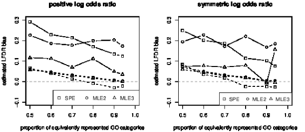
Figure 4: The performance of LFDR estimators for equivalently (dashed line) or differentially (solid line) represented GO categories.

Conclusions

Efron’s method [12, 13] can be used to estimate GO categories and thus address the gene enrichment problem, provided that thousands of GO categories are taken into account. However, in most gene enrichment studies, researchers focus on medium- or small-scale numbers of GO categories, i.e., several hundred, dozens or only one GO category. Here, we adapted $3$ LFDR estimators (the SPE, MLE, and NMLE) to address the gene enrichment problem with medium- and small-scale numbers of GO categories, and compared these using breast cancer and simulation data.

The MLE is sensitive to $k$, the number of PMM components. The MLE is used when considering a medium-scale number of GO categories, i.e., $100$. In our breast cancer data analysis, the estimated LFDRs of $\text{GO:}0051082$ and $\text{GO:}0005524$ using MLE2 were $100\%$ (Figure 1). However, the LFDRs estimated by MLE3 were very close to 0. Using the MLE formula shown in equation (17), and the $k$-component PMM shown in equation (14), we determined that the sensitivity of the LFDRs of GO category $i$ estimated by MLE2 and MLE3 depended mainly on the sensitivity of the Bayes factor, based on the number of PMM components. Comparing the probability masses of $\text{GO:}0005524$, based on the $2$- and $3$-component PMMs shown in Figure 2, we found that the probability mass of $\text{GO:}0005524$ under the null hypothesis is larger than that under the alternative hypothesis based on the $2$-component PMM (left plot in Figure 2). By contrast, the probability mass under the null hypothesis is smaller than that under the alternative hypothesis based on the $3$-component PMM (right plot in Figure 2). Thus, the LFDR estimated by the MLE is strongly dependent on the number of PMM components.

Nevertheless, the performance comparison in Figure 4 indicates that the MLE has lower bias than the SPE when the number of GO categories is much larger than $k$ even when the ideal value of $k$ is unknown. Moreover, MLE3 has lower bias than MLE2 as an LFDR estimator. However, when the number of GO categories is not much larger than $k$, the estimated proportion of GO categories equivalently represented become strongly biased toward $0$. In that situation, the false positive rate increases as the number of PMM components.

Due to its conservatism and freedom from the PMM, we recommend using the SPE when the number of GO categories of interest is too small for the MLE, e.g., about $10$ categories. Based on the simulations reported by Bickel [5], we conjecture that the SPE has acceptably low LFDR-estimation bias when there are at least 3 GO categories.

Finally, we recommend that the NMLE be used given only 1 or 2 GO categories of interest. Neither the MLE nor the SPE is able to estimate the LFDR for only $1$ GO category of interest; moreover, they probably have excessive bias when based on only $2$ GO categories. Thus, the NMLE is the recommended method of addressing the gene enrichment problem in this smallest-scale case. The NMLE depends not only on the data but also on a guess of the value of $\pi_{0}$, which, in the absence of strong prior information, is often set to the default value of 50%. A closely related approach is to use the NML ratio as an estimate of the Bayes factor directly without guessing $\pi_{0}$. By using 10 and 100 as thresholds of each estimated Bayes factor to determine whether a GO category is differentially represented, we reached similar conclusions whether using the NML and or an MLE (Figure 3). Thus, at least for our data set, the NML ratio tends to estimate the Bayes factor almost as accurately as methods that simultaneously use information across GO terms.

References

- Altshuler et al. [2008] D. Altshuler, M. J. Daly, and E. S. Lander. Genetic mapping in human disease. Science, 322:881–888, 2008. ISSN 0036-8075. doi: 10.1126/science.1156409.
- Barndorff-Nielsen and Cox [1994] O. E. Barndorff-Nielsen and D. R. Cox. Inference and Asymptotics. CRC Press, London, 1994.
- Benjamini and Hochberg [1995] Y. Benjamini and Y. Hochberg. Controlling the false discovery rate: A practical and powerful approach to multiple testing. Journal of the Royal Statistical Society B, 57:289–300, 1995.
- Bickel [2010] D. R. Bickel. Minimum description length methods of medium-scale simultaneous inference. Technical Report, Ottawa Institute of Systems Biology, arXiv:1009.5981v1, 2010.
- Bickel [2011a] D. R. Bickel. Simple estimators of false discovery rates given as few as one or two p-values without strong parametric assumptions. Technical Report, Ottawa Institute of Systems Biology, arXiv:1106.4490, 2011a.
- Bickel [2011b] D. R. Bickel. A predictive approach to measuring the strength of statistical evidence for single and multiple comparisons. Canadian Journal of Statistics, 39:610–631, 2011b.
- Bickel [2011c] D. R. Bickel. The strength of statistical evidence for composite hypotheses: Inference to the best explanation. Statistica Sinica DOI:10.5705/ss.2009.125 (online ahead of print), 2011c.
- Bickel [2011d] D. R. Bickel. Estimating the null distribution to adjust observed confidence levels for genome-scale screening. Biometrics, 67:363–370, 2011d.
- Bickel [2011e] D. R. Bickel. Small-scale inference: Empirical Bayes and confidence methods for as few as a single comparison. Technical Report, Ottawa Institute of Systems Biology, arXiv:1104.0341, 2011e.
- Dennis et al. [2003] G. Dennis, B. T. Sherman, D. A. Hosack, J. Yang, W. Gao, H. C. Lane, and R. A. Lempicki. DAVID: database for annotation, visualization, and integrated discovery. Genome Biology, 4(9), 2003.
- Doniger et al. [2003] S. W. Doniger, N. Salomonis, K. D. Dahlquist, K. Vranizan, S. C. Lawlor, and B. R. Conklin. MAPPFinder: using gene ontology and GenMAPP to create a global gene-expression profile from microarray data. Genome Biology, 4(1), 2003.
- Efron [2004] B. Efron. Large-scale simultaneous hypothesis testing: The choice of a null hypothesis. Journal of the American Statistical Association, 99(465):96–104, 2004.
- Efron [2010] B. Efron. Large-Scale Inference: Empirical Bayes Methods for Estimation, Testing, and Prediction. Cambridge University Press, Cambridge, 2010.
- Gentleman et al. [2005] R. Gentleman, V. Carey, W. Huber, R. Irizarry, and S. Dudoit, editors. Bioinformatics and Computational Biology Solutions Using R and Bioconductor. Springer, New York, 2005.
- Good [1966] I. J. Good. How to Estimate Probabilities. IMA Journal of Applied Mathematics, 2:364–383, 1966. doi: 10.1093/imamat/2.4.364.
- Grünwald [2007] P. D. Grünwald. The Minimum Description Length Principle. MIT Press, London, 2007.
- Hong et al. [2009] W.-J. Hong, R. Tibshirani, and G. Chu. Local false discovery rate facilitates comparison of different microarray experiments. Nucleic Acids Research, 37(22):7483–7497, 2009.
- Huang et al. [2009] D.W. Huang, B.T. Sherman, and R.A. Lempicki. Bioinformatics enrichment tools: paths toward the comprehensive functional analysis of large gene lists. Nucleic Acids Research, 37(1):1–13, 2009.
- Jeffreys [1948] H. Jeffreys. Theory of Probability. Oxford University Press, London, 1948.
- Kanehisa and Goto [2000] M. Kanehisa and S. Goto. KEGG: Kyoto Encyclopedia of Genes and Genomes. Nucleic Acids Research, 28(1):27–30, 2000.
- Khatri et al. [2002] P. Khatri, S. Draghici, G. C. Ostermeier, and S. A. Krawetz. Profiling gene expression using onto-express. Genomics, 79(2):266–270, 2002.
- Min et al. [2010] J. L. Min, A. Barrett, T. Watts, F. H. Pettersson, H. E. Lockstone, C. M. Lindgren, J. M. Taylor, M. Allen, K. T. Zondervan, and M. I. McCarthy. Variability of gene expression profiles in human blood and lymphoblastoid cell lines. BMC Genomics, 11(1), 2010.
- Muralidharan [2010] Omkar Muralidharan. An empirical Bayes mixture method for effect size and false discovery rate estimation. Annals of Applied Statistics, 4:422–438, 2010.
- Pawitan et al. [2005] Y. Pawitan, K.R.K. Murthy, S. Michiels, and A. Ploner. Bias in the estimation of false discovery rate in microarray studies. Bioinformatics, 21:3865–3872, 2005.
- Reyal et al. [2008] F. Reyal, M. H. van Vliet, N. J. Armstrong, H. M. Horlings, K. E. de Visser, M. Kok, A. E. Teschendorff, S. Mook, L. van ’t Veer, C. Caldas, R. J. Salmon, M. J. V. D. Vijver, and L. F. A. Wessels. A comprehensive analysis of prognostic signatures reveals the high predictive capacity of the proliferation, immune response and RNA splicing modules in breast cancer. Breast Cancer Research, 10(6), 2008.
- Scholtens et al. [2004] D. Scholtens, A. Miron, F. M. Merchant, A. Miller, P. L. Miron, J. D. Iglehart, and R. Gentleman. Analyzing factorial designed microarray experiments. Journal of Multivariate Analysis, 90(1 SPEC. ISS.):19–43, 2004.
- Severini [2000] T.A. Severini. Likelihood Methods in Statistics. Oxford University Press, Oxford, 2000.
- Storey [2003] J. D. Storey. The positive false discovery rate: A Bayesian interpretation and the q-value. Annals of Statistics, 31(6):2013–2035, 2003.
- Wang et al. [2011] R.-L. Wang, D. Bencic, J. Lazorchak, D. Villeneuve, and G. T. Ankley. Transcriptional regulatory dynamics of the hypothalamic-pituitary-gonadal axis and its peripheral pathways as impacted by the 3-beta HSD inhibitor trilostane in zebrafish (danio rerio). Ecotoxicology and Environmental Safety, 74(6):1461–1470, 2011.
- Yang and Bickel [2010] Y. Yang and D. R. Bickel. Minimum description length and empirical Bayes methods of identifying SNPs associated with disease. Technical Report, Ottawa Institute of Systems Biology, COBRA Preprint Series, Article 74, biostats.bepress.com/cobra/ps/art74, 2010.
- Zeeberg et al. [2003] B. R. Zeeberg, W. Feng, G. Wang, M. D. Wang, A. T. Fojo, M. Sunshine, S. Narasimhan, D. W. Kane, W. C. Reinhold, S. Lababidi, K. J. Bussey, J. Riss, J. C. Barrett, and J. N. Weinstein. Gominer: a resource for biological interpretation of genomic and proteomic data. Genome Biology, 4(4), 2003.