Abstract

By using the gauge/gravity duality and the Maldacena prescription we compute the expectation values of the Wilson loops in hot, noncommutative Yang-Mills (NCYM) theory in (3+1) dimensions. We consider both the time-like and the light-like Wilson loops. The gravity dual background is given by a particular decoupling limit of non-extremal (D1,D3) bound state of type IIB string theory. We obtain the velocity dependent quark-antiquark potential and numerically study how the dipole length and the potential change with velocity (for $0<v<1$, i.e., the Wilson loop is time-like) of the dipole as well as noncommutativity. We discuss and compare the results with the known commutative results. We also obtain an analytic expression for the screening length when the rapidity is large and the noncommutativity parameter is small with the product remaining small. When $v\to 1$, the time-like Wilson loop becomes light-like and in that case we obtain the form of the jet quenching parameter for the strongly coupled noncommutative Yang-Mills plasma which matches with our earlier results obtained using different approach.

1 Introduction

One of the remarkable features of AdS/CFT correspondence [1, 2, 3] and its generalizations [4] is that it gives us access to the non-perturbative regimes of large $N$ gauge theories simply from the low energy, weakly coupled string theory in certain backgrounds. So, for example, the expectation values of Wilson loops, which are non-perturbative objects in gauge theories, can be computed using AdS/CFT correspondence as has been prescribed in [5, 6, 7, 8]. In strongly coupled gauge theories of interacting quark-gluon plasma, Wilson loops can be related to various measurable quantities in heavy ion experiments in RHIC or in LHC. For example, the expectation value of a special time-like Wilson loop can be related to the static quark-antiquark potential [9] in a moving quark-gluon plasma. On the other hand, the expectation value of a particular light-like Wilson loop can be related, among other things, to the radiative energy loss of a parton or the jet quenching parameter [10].

The velocity dependent quark-antiquark potential of a dipole moving with an arbitrary velocity through the hot quark-gluon plasma including the screening length [11, 12, 13, 14] as well as the jet quenching parameter [15, 16] have been calculated when the plasma is described by $D=4$, ${\cal N}=4$, SU($N$) Yang-Mills theory using AdS/CFT correspondence. In this paper we calculate the velocity dependent quark-antiquark potential, the screening length and the jet quenching parameter when the plasma is described by $D=4$, thermal, noncommutative Yang-Mills (NCYM) theory at large $N$ using gauge/gravity duality. NCYM theory arises quite naturally in string theory [27, 28, 29] and M-theory [30] and it is of interest to see how noncommutativity affects the known velocity dependent quark-antiquark potential, screening length as well as the jet quenching parameter of the ordinary super YM theory.

The gravity background in this case is given by a particular decoupling limit [28] of non-extremal (D1, D3) bound state system of type IIB string theory. (D1, D3) bound state [31, 32] contains a non-zero $B$-field and it becomes asymptotically very large in the decoupling limit and is the source of space-space noncommutativity [27]. We use the string probe in this background and extremize the Nambu-Goto string world-sheet action in a particular static gauge and in turn obtain the expectation value of the Wilson loop, where the loop is the boundary of the above minimal area. We consider both the time-like and the light-like Wilson loops. From the time-like Wilson loop, we calculate the velocity dependent quark-antiquark potential, when the background or the plasma is moving with a velocity $v$ (for $0<v<1$) and the end-points of the fundamental string act as a heavy quark-antiquark pair or a dipole in the boundary gauge theory. We will take the background (or the plasma) to be moving along one of the brane directions (which is taken to be a commutative direction) relative to the dipole which lies along one of the noncommutative directions. There are other possibilities, but this is the simplest case where the noncommutative effect shows up. The quark-antiquark potential obtained from the minimal area of the world-sheet can only be given numerically. We first plot the dipole length as a function of certain constants of motion and then using this we plot the potential as a function of the dipole length at different velocities and noncommutativity parameters. The results are compared with the known commutative case [16]. We also give an analytic expression for the screening length when the rapidity is large and the noncommutativity parameter is small with the product also remaining small. Finally, for the completeness, we consider the case where the velocity $v\to 1$ and the time-like Wilson loop becomes light-like. In this case we recover the form of the jet quenching parameter as obtained before [33] using a different approach.

This paper is organized as follows. In section 2, we compute the time-like Wilson loop and give our numerical results for the dipole length and the quark-antiquark potential. We also obtain the analytic form of the screening length in some spacial case. In section 3, we take the velocity to unity and obtain the light-like Wilson loop. From this we obtain the form of the jet quenching parameter in this theory. Finally, we conclude in section 4.

2 Time-like Wilson Loop and $Q$-$\bar{Q}$ potential

In this section we will compute the time-like Wilson loop for the hot noncommutative Yang-Mills theory in (3+1)-dimensions from gauge/gravity duality. The gravity dual of noncommutative Yang-Mills theory is given by a particular decoupling limit [28, 29] of the non-extremal (D1, D3) bound state of type IIB string theory. We use the fundamental string as a probe in this background and compute the Nambu-Goto string world-sheet action. This action is then extremized to relate it to the expectation value of the time-like Wilson loop [16]. We will study numerically both the separation length of the quark-antiquark and the potential when we vary the velocity and the noncommutativity parameter. We will also give an analytic expression of the screening length in some special limit.

The non-extremal (D1, D3) bound state solution of type IIB string theory is given by the following metric (given in the string frame), the dilaton, the NSNS $B$-field and the RR form-fields [32],

$$ds^{2} = H^{-\frac{1}{2}}\left(-f(dt)^{2}+(dx^{1})^{2}+\frac{H}{F}\left((dx^{2})^{2}+(dx^{3})^{2}\right)\right)+H^{\frac{1}{2}}\left(\frac{dr^{2}}{f}+r^{2}d\Omega_{5}^{2}\right)$$

$$e^{2\phi} = g_{s}^{2}\frac{H}{F},\qquad B_{23}=\frac{\tan\alpha}{F}$$

$$A_{01} = \frac{1}{g_{s}}(H^{-1}-1)\sin\alpha\coth\varphi,\qquad A_{0123}=\frac{1}{g_{s}}\frac{(1-H)}{F}\cos\alpha\coth\varphi+{\rm T.\,T.}$$ (1)

where the various functions appearing above are,

$$f=1-\frac{r_{0}^{4}}{r^{4}},\qquad H=1+\frac{r_{0}^{4}\sinh^{2}\varphi}{r^{4}},\qquad F=1+\frac{r_{0}^{4}\cos^{2}\alpha\sinh^{2}\varphi}{r^{4}}$$ (2)

Here D3-branes lie along $x^{1},\,x^{2},\,x^{3}$ and D1-branes lie along $x^{1}$. The angle $\alpha$ measures the relative number of D1 and D3 branes by the relation $\cos\alpha=N/\sqrt{N^{2}+M^{2}}$, where $N$ is the number of D3-branes and $M$ is the number of D1-branes per unit codimension two surface transverse to D1-branes [34]. Also in the above $\varphi$ is the boost parameter and $r_{0}$ is the radius of the horizon of the non-extremal (D1, D3) bound state solution. $\phi$ is the dilaton and $g_{s}$ is the string coupling constant. $A_{01}$ and $A_{0123}$ are the RR form-fields corresponding to D1-brane and D3-brane respectively. T.T. denotes a term, involving transverse part of the brane to make the field-strength self-dual, whose explicit form is not required for our discussion. $B_{23}$ is the NSNS form responsible for the appearance of noncommutativity in the decoupling limit.

The NCYM decoupling limit is a low energy limit for which we zoom into the region [28],

$$r_{0}<r\sim r_{0}\sqrt{\sinh\varphi\cos\alpha}\ll r_{0}\sqrt{\sinh\varphi}$$ (3)

The above limit implies that $\varphi$ is a large parameter and the angle $\alpha$ is close to $\pi/2$. In this limit we get,

$$H\approx\frac{r_{0}^{4}\sinh^{2}\varphi}{r^{4}},\qquad\frac{H}{F}\approx\frac{1}{\cos^{2}\alpha(1+a^{4}r^{4})}\equiv\frac{h}{\cos^{2}\alpha}$$ (4)

where we have defined

$$h\equiv\frac{1}{1+a^{4}r^{4}},\qquad{\rm with},\quad a^{4}\equiv\frac{1}{r_{0}^{4}\sinh^{2}\varphi\cos^{2}\alpha}$$ (5)

From (2) we notice that since the asymptotic value of $B$-field is $\tan\alpha$ and $\alpha\to\pi/2$ in the decoupling limit, the $B$-field becomes very large. The non-vanishing component of the $B$-field is $B_{23}$ which gives rise to a magnetic field in the D3-brane world-volume and is responsible for making $x^{2}$ and $x^{3}$ directions noncommutative [35]. Using (4), we rewrite the metric in (2) as,

$$ds^{2}=\frac{r^{2}}{r_{0}^{2}\sinh\varphi}\left(-fdt^{2}+(dx^{1})^{2}+h\left[(dx^{2})^{2}+(dx^{3})^{2}\right]\right)+\frac{r_{0}^{2}\sinh\varphi}{r^{2}}\left(\frac{dr^{2}}{f}+r^{2}d\Omega_{5}^{2}\right)$$ (6)

Here the function $h$ is as defined in (5) and also in writing (6) we have rescaled the coordinates as, $x^{2,\,3}\to\cos\alpha x^{2,\,3}$. This metric along with the other field configurations given in (2) in the NCYM decoupling limit is the gravity dual of four dimensional thermal NCYM theory. We use fundamental open string as a probe and consider its dynamics in this background. Let the line joining the end points of the string or the dipole lie along $x^{2}$ one of the noncommutative directions and move along $x^{1}$ with a velocity $v$ where $0<v<1$ . To simplify the calculation we can go to the rest frame $(t^{\prime},\,x^{1}\,{}^{\prime})$ of the dipole by boosting the coordinate as,

$$dt = \cosh\eta dt^{\prime}-\sinh\eta dx^{1}\,{}^{\prime}$$

$$dx^{1} = -\sinh\eta dt^{\prime}+\cosh\eta dx^{1}\,{}^{\prime}$$ (7)

where the rapidity $\eta$ is related to $v$ as $\tanh\eta=v$. So, in this frame the dipole is static and the background (or the plasma) is moving with a velocity $v$ in the negative $x^{1}$-direction. Note that the rectangular Wilson loop lies along $t^{\prime}$ and $x^{2}$ directions and we denote the lengths along those directions as ${\cal T}$ and $L$ respectively. We also assume ${\cal T}\gg L$ such that the string world-sheet is time translation invariant. Using (2) in the metric (6) we get,

$$ds^{2} = -A(r)dt^{2}-2B(r)dtdx^{1}+C(r)(dx^{1})^{2}+\frac{r^{2}h}{r_{0}^{2}\sinh\varphi}\left[(dx^{2})^{2}+(dx^{3})^{2}\right]$$ (8)

$$\qquad\qquad\qquad+\frac{r_{0}^{2}\sinh\varphi}{r^{2}}\frac{dr^{2}}{f}+r_{0}^{2}\sinh\varphi d\Omega_{5}^{2}$$

$$= G_{\mu\nu}dx^{\mu}dx^{\nu}$$

where

$$A(r) = \frac{r^{2}}{r_{0}^{2}\sinh\varphi}\left(1-\frac{r_{0}^{4}\cosh^{2}\eta}{r^{4}}\right)$$

$$B(r) = \frac{r_{0}^{2}\sinh\eta\cosh\eta}{r^{2}\sinh\varphi}$$

$$C(r) = \frac{r^{2}}{r_{0}^{2}\sinh\varphi}\left(1+\frac{r_{0}^{4}\sinh^{2}\eta}{r^{4}}\right)$$ (9)

Note that since we will be using the ‘primed’ coordinates from now on, we have dropped the prime for simplicity. We will evaluate the Nambu-Goto action of the string world-sheet in this background. The Nambu-Goto action is given as,

$$S=\frac{1}{2\pi\alpha^{\prime}}\int d\sigma d\tau\sqrt{-{\rm det}\,g_{\alpha\beta}}$$ (10)

where $g_{\alpha\beta}$ is the induced metric on the world-sheet given as

$$g_{\alpha\beta}=G_{\mu\nu}\frac{\partial x^{\mu}}{\partial\xi^{\alpha}}\frac{\partial x^{\nu}}{\partial\xi^{\beta}}$$ (11)

with $G_{\mu\nu}$ is as given in (8). In the above $\xi^{\alpha}$ are the world-sheet coordinates $\tau$ and $\sigma$ for $\alpha=0$ and $\alpha=1$ respectively. We choose the static gauge for evaluating (10) as, $\tau=t$, $\sigma=x^{2}$, where $-L/2\leq x^{2}\leq L/2$ and $r=r(\sigma)$, $x^{1}(\sigma)=x^{3}(\sigma)=$ constant. $r(\sigma)$ is the string embedding we want to determine by extremizing the Nambu-Goto action, with the boundary condition $r(\pm L/2)=r_{0}\Lambda$ (here $\Lambda$ is a parameter). Using these in the action (8), we get,

$$S=\frac{{\cal T}}{2\pi\alpha^{\prime}}\int_{-L/2}^{L/2}d\sigma\left[A(r)\left(\frac{r^{2}h}{r_{0}^{2}\sinh\varphi}+\frac{r_{0}^{2}\sinh\varphi}{r^{2}}\frac{\left(\partial_{\sigma}r\right)^{2}}{f}\right)\right]^{\frac{1}{2}}$$ (12)

with $A(r)$ as given in (2). Introducing dimensionless quantities $y=r/r_{0}$, $\tilde{\sigma}=\sigma/(r_{0}\sinh\varphi)$ and $\ell=L/(r_{0}\sinh\varphi)$, the Nambu-Goto action (12) can be rewritten as,

$$S=\frac{{\cal T}r_{0}}{\pi\alpha^{\prime}}\int_{0}^{\ell/2}d\sigma{\cal L}={\cal T}T\sqrt{\hat{\lambda}}\int_{0}^{\ell/2}d\sigma{\cal L}$$ (13)

where

$${\cal L}=\sqrt{\left(y^{4}-\cosh^{2}\eta\right)\left(\frac{1}{1+a^{4}r_{0}^{4}y^{4}}+\frac{y^{\prime 2}}{y^{4}-1}\right)}$$ (14)

Note that we have removed ‘tilde’ from $\tilde{\sigma}$ while writing (13) as it is an integration variable. Also $y^{\prime}$ denotes $dy/d\sigma$ and we have used the fact that $y$ is an even function of $\sigma$ by symmetry. In writing the second expression in (13) we have made use of the standard gauge/gravity relation [28, 29],

$$T=\frac{1}{\pi r_{0}\cosh\varphi}\approx\frac{1}{\pi r_{0}\sinh\varphi},\qquad r_{0}^{4}\sinh^{2}\varphi=2\hat{g}_{\rm YM}^{2}N\alpha^{\prime 2}=\hat{\lambda}\alpha^{\prime 2}$$

$${\rm and}\quad a^{4}r_{0}^{4}\equiv\frac{1}{\sinh^{2}\varphi\cos^{2}\alpha}=\pi^{4}\hat{\lambda}T^{4}\theta^{2}$$ (15)

The first relation in (2) is obtained from calculating the Hawking temperature of the non-extremal (D1, D3) brane given by the metric in (2) (note that in the decoupling limit when $\varphi$ is large $\cosh\varphi\approx\sinh\varphi$) and this is the temperature of the NCYM theory by gauge/gravity duality. The second relation is obtained from the D3-brane charge where $N$ is the number of D3-branes and in NCYM theory this is the rank of the gauge group. $\hat{g}_{\rm YM}$ is the NCYM coupling and $2\hat{g}_{\rm YM}^{2}N=\hat{\lambda}$ is the ’t Hooft coupling of the NCYM theory. The NCYM ’t Hooft coupling is related to the ordinary ’t Hooft coupling by the relation $\lambda=(\alpha^{\prime}/\theta)\hat{\lambda}$, where $\theta$ is the noncommutativity parameter defined by $[x^{2},\,x^{3}]=i\theta$ [28]. Here $\theta$ is a finite parameter and in the decoupling limit as $\alpha^{\prime}\to 0$, $\hat{\lambda}$ remains finite. The third relation is obtained using the first two and also using $\cos\alpha=\alpha^{\prime}/\theta$ in the decoupling limit. Note that in the decouping limit as $\alpha^{\prime}\to 0$, $\alpha\to\pi/2$ as mentioned earlier. We will compute $y(\sigma)$ by extremizing the action (13).

Now since the Lagrangian density in (13) does not explicitly depend on $\sigma$, we have the following constant of motion,

$${\cal H}={\cal L}-y^{\prime}\frac{\partial{\cal L}}{\partial y^{\prime}}=\frac{y^{4}-\cosh^{2}\eta}{(1+a^{4}r_{0}^{4}y^{4})\sqrt{(y^{4}-\cosh^{2}\eta)\left(\frac{1}{1+a^{4}r_{0}^{4}y^{4}}+\frac{y^{\prime 2}}{y^{4}-1}\right)}}=q={\rm const.}$$ (16)

As in the commutative theory [16] we will consider two cases: (a) $\sqrt{\cosh\eta}<\Lambda$ and then take $\Lambda\to\infty$. The rapidity in this case remains finite, the Wilson loop is time-like and the action is real. We will compute the quark-antiquark potential in this case and also give an expression of screening length in some special case. (b) $\sqrt{\cosh\eta}>\Lambda$ and then take $\eta\to\infty$, keeping $\Lambda$ finite. The Wilson loop in this case is light-like and the action is imaginary. We will take $\Lambda\to\infty$ in the end and obtain the expression of the jet quenching parameter for the noncommutative hot Yang-Mills plasma.

We will consider case (a) in this section and case (b) in the next section. When $\sqrt{\cosh\eta}<\Lambda$, the action would be real and from (16) $y^{\prime}$ can be solved as,

$$y^{\prime}=\frac{\sqrt{1-a^{4}r_{0}^{4}q^{2}}}{q(1+a^{4}r_{0}^{4}y^{4})}\sqrt{(y^{4}-1)\left(y^{4}-y_{c}^{4}\right)}$$ (17)

where $y_{c}^{4}=(\cosh^{2}\eta+q^{2})/(1-a^{4}r_{0}^{4}q^{2})>1$ denotes the larger turning point where $y^{\prime}$ vanishes. Integrating (17) we obtain,

$$2\int_{0}^{\ell/2}d\sigma=\ell(q)=\frac{2q}{\sqrt{1-a^{4}r_{0}^{4}q^{2}}}\int_{y_{c}}^{\Lambda}\frac{1+a^{4}r_{0}^{4}y^{4}}{\sqrt{(y^{4}-1)(y^{4}-y_{c}^{4})}}dy$$ (18)

We remark that if we naively take $\Lambda$, where the boundary theory is supposed to live to $\infty$, the above integral diverges. Here $\ell$ is related to the dipole length $L$ by $\ell=L/(r_{0}\sinh\varphi)=\pi LT$ and so the divergence in $\ell(q)$ is physically meaningless. Note that $\ell(q)$ in the commutative theory is indeed finite as can be seen from (18) by putting $a^{2}r_{0}^{2}\sim\theta$, which is a measure of noncommutativity, to zero. However, for the noncommutative case $\ell(q)$ is divergent if we take $\Lambda\to\infty$. The reason is that the noncommutative gauge theory does not live at $\Lambda=\infty$, but at some finite value of $\Lambda$, whose exact value is not known. This is implicit in [28]. It has been shown there that in a noncommutative theory it is not possible to fix the position of the string end point at infinity as a small perturbation would change it violently. This has also been explicitly mentioned in [36].

In the context of a Wilson loop calculation, it has been noticed before [37] that the string end points for a static string can not be fixed at a finite length at $\Lambda\to\infty$ in a noncommutative theory. Therefore, the dipole length $L$ indeed diverges. The reason for this divergence has been argued to be the non-local interaction between the $Q$-$\bar{Q}$ pair in a magnetic field [38]. To be precise, the interaction point in terms of the center of mass coordinate gets shifted by a momentum dependent term. Thus if the only non-zero component of the $B$-field is $B_{23}$, as in our case, then by placing the dipole along $x^{2}$, it automatically gets a momentum along $x^{3}$. So, if we keep the dipole static along $x^{3}$, the length will diverge at infinity. To compensate the momentum along $x^{3}$, the dipole must move along $x^{3}$ with a particular velocity [39]. In that case, the end points of the string can be fixed at a finite length on the boundary at infinity and thus the divergence in the dipole length gets removed.

In the following, we, however, remove the divergence in the dipole length in a different way. We have noticed in (18), the integral representation of the dipole length, that by explicit evaluation the integral diverges (note that the dipole in our case does not move along $x^{3}$) as we take $\Lambda\to\infty$. But, the integral can be regularized to give a finite result if we can explicitly extract the divergent term (the part that goes to infinity as $\Lambda\to\infty$) of the integral and remove it. After regularization, the noncommutative theory may be thought of as living at $\Lambda=\infty$. So, after regularization we will take $\Lambda\to\infty$. It is not difficult to obatin the divergent term from the integral (18) when $\Lambda\to\infty$ and by inspection it can be seen to have the form $2qa^{4}r_{0}^{4}\Lambda/\sqrt{1-a^{4}r_{0}^{4}q^{2}}$. Subtracting the divergent part the finite $\ell(q)$ can be written in the integral form as,

$$\ell(q)=\frac{2q}{\sqrt{1-a^{4}r_{0}^{4}q^{2}}}\left.\left[\int_{y_{c}}^{\Lambda}\frac{1+a^{4}r_{0}^{4}y^{4}}{\sqrt{(y^{4}-1)(y^{4}-y_{c}^{4})}}dy-a^{4}r_{0}^{4}\Lambda\right]\right|_{\Lambda\to\infty}$$ (19)

The above equation therefore gives us the quark antiquark separation $L(q)=\ell(q)/(\pi T)$ of the dipole as a function of the constant of motion $q$. It is not possible to perform the integration in (19) and give an analytic expression of $\ell(q)$. So, we will perform the integration numerically for different fixed values of the rapidity $\eta$ and the noncommutativity parameter $ar_{0}\sim\hat{\lambda}^{1/4}T\sqrt{\theta}$ and use this to evaluate the quark-antiquark potential. However, we can give the analytic expression of $\ell(q)$ and the screening length only for some special values of the rapidity and the noncommutativity parameter which will be discussed later.

Now substituting $y^{\prime}$ from (17) into the action (13) we get,

$$S(\ell)=\frac{{\cal T}T\sqrt{\hat{\lambda}}}{\sqrt{1-a^{4}r_{0}^{4}q^{2}}}\int_{y_{c}}^{\Lambda}\frac{y^{4}-\cosh^{2}\eta}{\sqrt{(y^{4}-1)(y^{4}-y_{c}^{4})}}dy$$ (20)

However, as it is known [16] from the commutative case that this action is divergent as we take $\Lambda\to\infty$. The reason for this divergence for the commutative case is that this action contains the quark-antiquark self-energy $S_{0}$ and once this is subtracted from $S(\ell)$, the action becomes finite and from there one calculates the potential. In the noncommutative case also, we need to subtract the quark-antiquark self energy $S_{0}$. This is calculated by evaluating the Nambu-Goto action for the single string stretched between the horizon $r_{0}$ and the boundary at $r_{0}\Lambda$ and then multiply by 2 (for the two strings associated with quark and antiquark). The Nambu-Goto action in this case is evaluated by considering a quark moving in the $x^{1}$-direction (which is commutative) and so, the gauge condition one uses is $\tau=t$, $\sigma=r$, $x^{1}=x^{1}(\sigma)$, $x^{2}(\sigma)=x^{3}(\sigma)=$ constant. However, since $x^{2}$ and $x^{3}$ are the noncommutative directions the computation of $S_{0}$ remains unaffected by the noncommutativity. Therefore, $S_{0}$ takes exactly the same form as evaluated in the commutative case given as [16]

$$S_{0}={\cal T}T\sqrt{\hat{\lambda}}\int_{1}^{\Lambda}dy$$ (21)

So, subtracting $S_{0}$ from $S(\ell)$ we get,

$$S(\ell)-S_{0} = \frac{{\cal T}T\sqrt{\hat{\lambda}}}{\sqrt{1-a^{4}r_{0}^{4}q^{2}}}\left[\int_{y_{c}}^{\Lambda}dy\left\{\frac{y^{4}-\cosh^{2}\eta}{\sqrt{(y^{4}-1)(y^{4}-y_{c}^{4})}}-\sqrt{1-a^{4}r_{0}^{4}q^{2}}\right\}\right.$$ (22)

$$\qquad\qquad\qquad\qquad\qquad\qquad\qquad\left.-\sqrt{1-a^{4}r_{0}^{4}q^{2}}(y_{c}-1)\right]$$

It is clear from (22) that in the commutative case when $a^{2}r_{0}^{2}\sim\theta$ is put to zero, $S(\ell)-S_{0}$ is indeed finite when we take $\Lambda\to\infty$. However, this is not the case when noncommutativity is present. The reason is, as we mentioned before, the NCYM theory does not live at $\Lambda=\infty$, but at a finite $\Lambda$ [28, 36]. (Another way of understanding this divergence has been mentioned earlier from the arguments given in [37, 38, 39].) So, we will subtract the divergent term from (22) and then take $\Lambda\to\infty$. Doing that we find the finite quark-antiquark potential as,

$$E(\ell) = \frac{S-S_{0}-S_{\rm div}}{\cal T}$$ (23)

$$= \frac{T\sqrt{\hat{\lambda}}}{\sqrt{1-a^{4}r_{0}^{4}q^{2}}}\left[\int_{y_{c}}^{\Lambda}dy\left\{\frac{y^{4}-\cosh^{2}\eta}{\sqrt{(y^{4}-1)(y^{4}-y_{c}^{4})}}-\sqrt{1-a^{4}r_{0}^{4}q^{2}}\right\}\right.$$

$$\qquad\qquad\qquad\left.\left.-\sqrt{1-a^{4}r_{0}^{4}q^{2}}(y_{c}-1)-\left(1-\sqrt{1-a^{4}r_{0}^{4}q^{2}}\right)\Lambda\right]\right|_{\Lambda\to\infty}$$

where in the above $S_{\rm div}$ is $(1-\sqrt{1-a^{4}r_{0}^{4}q^{2}})\Lambda$ with $\Lambda\to\infty$. Here also it is not possible to perform the integration in (23) in a closed form. So, we will obtain the quark-antiquark potential numerically. We first plot $\ell(q)$ vs. $q$ using (19) and use it to plot $E(\ell)$ vs. $\ell$ from (23) at different fixed values of the rapidity $\eta$ and the noncommutativity parameter $ar_{0}$.

2.1 Plots and discussion of the results

In this subsection we give and discuss the various plots of quark-antiquark separation $\ell(q)$ as a function of constant of motion $q$ and the velocity dependent quark-antiquark potential $E(\ell)$ as a function of the quark-antiquark separation length $\ell$ for various values of the rapidity ($\eta$) as well as the noncommutativity parameter ($ar_{0}\sim\sqrt{\theta}$).

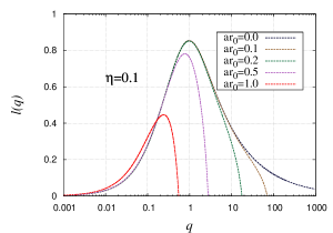
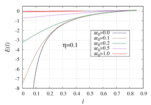
Figure 1: (a) shows the plot of the quark-antiquark separation $\ell(q)$ as a function of the const. of motion $q$ for different values of the noncommutativity parameter $ar_{0}$, when the rapidity is kept fixed at $\eta=0.1$. (b) shows the plot of the properly normalized quark-antiquark potential $E(\ell)$ as a function of $\ell$ for the same set of values of the noncommutativity parameter with the same value of $\eta=0.1$.

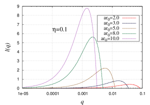
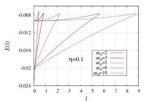
Figure 2: (a) shows the plot of the quark-antiquark separation $\ell(q)$ as a function of the const. of motion $q$ for different values (but larger than those given in Figure 1) of the noncommutativity parameter $ar_{0}$ with the same $\eta=0.1$ as in Figure 1. (b) shows the plot of the properly normalized quark-antiquark potential $E(\ell)$ as a function of $\ell$ for the same set of values of the noncommutativity parameter with the same $\eta=0.1$.

Note that each figure contains two parts (a) and (b). While in (a) we plot $\ell(q)$ vs $q$, in (b) we plot the quark-antiquark potential $E(\ell)$ vs $\ell$. In plot (b) we make use of plot (a) to obtain $q$ for each value of $\ell(q)$. Generically in all these figures the $\ell(q)$ in part (a) starts at zero for $q=0$ (in fact for small $q$, $\ell(q)\to 0$ as $q$ which can be seen from (19)) and as $q$ increases it ends at zero either at a finite value of $q$, denoted as $q_{\rm max}$, (when noncommutativity is present or $ar_{0}\neq 0$) or at $q\to\infty$ (when there is no noncommutativity or $ar_{0}=0$) (for large $q$, $\ell(q)\to 0$ as $q^{-1/2}$ which can be seen again from (19)). In between, $\ell(q)$ has a single maximum at some finite $q<q_{\rm max}$ indicating that there exists a screening length (proportional to $\ell_{\rm max}$) beyond which there is no solution to (19). So, given a curve, there is an $\ell_{\rm max}$ beyond which there is no dipole solution, that is, the dipole dissociates and below $\ell_{\rm max}$ there are two dipoles at a fixed $\ell$ for two different values of $q$. Accordingly, $E(\ell)$ or $Q$-${\bar{Q}}$ potential in part (b) generically in all the figures have two branches corresponding to the dipoles with two different values of $q$. The smaller value of $q$ corresponds to the upper branch and the dipole has higher energy, whereas, the larger value of $q$ corresponds to the lower branch and the dipole has lower energy. So, the dipole with lower $q$ will be metastable and will go to the state with higher $q$ as it is energetically more favorable.

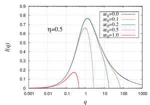
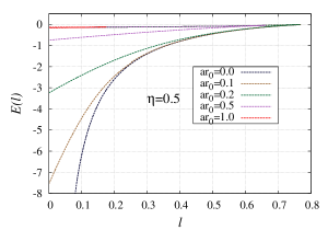
Figure 3: (a) shows the plot of the quark-antiquark separation $\ell(q)$ as a function of the const. of motion $q$ for different values of the noncommutativity parameter $ar_{0}$, but now the rapidity is kept fixed at $\eta=0.5$. (b) shows the plot of the properly normalized quark-antiquark potential $E(\ell)$ as a function of $\ell$ for the same set of values of the noncommutativity parameter with the same value of $\eta=0.5$

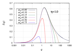
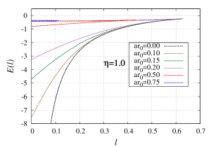
Figure 4: (a) shows the plot of the quark-antiquark separation $\ell(q)$ as a function of the const. of motion $q$ for different values of the noncommutativity parameter $ar_{0}$, but now the rapidity is fixed at $\eta=1.0$. (b) shows the plot of the properly normalized quark-antiquark potential $E(\ell)$ as a function of $\ell$ for the same set of values of the noncommutative parameter with the same $\eta=1.0$.

Also from part (b) we note that there exists a critical value of the rapidity $\eta_{c}$ (whose value changes with the value of the noncommutativity parameter), beyond which the entire upper branch of the $E(\ell)$ curve is negative. However, below this value, i.e., $\eta<\eta_{c}$, the $E(\ell)$ curve crosses zero at $\ell=\ell_{c}$, continues to rise till $\ell=\ell_{\rm max}$ and then turns back crossing zero again at $\ell=\ell_{c}^{\prime}>\ell_{c}$. There are various portions of the $E(\ell)$ vs $\ell$ curve, namely, $\ell<\ell_{c}$, $\ell=\ell_{c}$, $\ell_{c}<\ell<\ell_{c}^{\prime}$, $\ell=\ell_{c}^{\prime}$, $\ell_{c}^{\prime}<\ell<\ell_{\rm max}$ and $\ell>\ell_{\rm max}$ which need separate discussions as far as the quark-antiquark potential is concerned. However, the discussion is pretty much the same as in the commutative case given in [16, 40] and will not be repeated here. We will point out the differences due to noncommutativity as we go along.

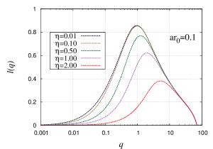
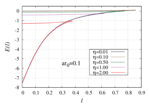
Figure 5: (a) shows the plot of quark-antiquark separation $\ell(q)$ as a function of the const. of motion $q$ for different values of the rapidity $\eta$ with the noncommutativity parameter kept fixed at $ar_{0}=0.1$. (b) shows the plot of the properly normalized quark-antiquark potential $E(\ell)$ as a function of $\ell$ for the same set of values of the rapidity with the same $ar_{0}=0.1$.

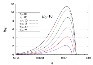
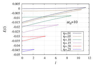
Figure 6: (a) shows the plot of the quark-antiquark separation $\ell(q)$ as a function of the const. of motion $q$ for different values of the rapidity $\eta$ but now the noncommutativity parameter is kept fixed at a much larger value $ar_{0}=10.0$. (b) shows the plot of the properly normalized quark-antiquark potential $E(\ell)$ as a function of $\ell$ for the same set of values of the rapidity with the same $ar_{0}=10.0$.

In Figures 1 and 2, the rapidity is fixed at $\eta=0.1$. However, in Figure 1 the noncommutativity parameter $ar_{0}$ takes small values starting from $0.0$ (where there is no noncommutativity) to $1.0$, whereas, in Figure 2 the noncommutativity parameter takes fairly large values starting from $2.0$ to $10.0$. The main difference between the commutative results and the noncommutative results is that in the former case the constant of motion $q$ can take arbitrarily large values, but in the latter case $q$ can not exceed certain finite value ($q_{\rm max}$) because beyond this value the quark-antiquark separation $\ell(q)$ becomes negative which is unphysical. The reason behind this cut-off is the regularization of the integral made in (19). Note that the last term in (19) is subtracted in order to make $\ell(q)$ finite as $\Lambda\to\infty$. However, as $q$ increases, $y_{c}$ increases which makes the last term dominate over the integral and therefore $\ell(q)$ becomes negative. Thus this effect is due to the noncommutativity of the underlying boundary theory. We see from Figure 1(a) that as the noncommutativity parameter $ar_{0}$ increases, $\ell(q)$ curve deviates more and more from the commutative curve, the $\ell_{\rm max}$ falls and the peak shifts towards the left (i.e., the maximum occurs at a smaller value of $q$). In particular, the deviation from the commutative case becomes more pronounced after $\ell_{\rm max}$ is reached. However this feature continues upto certain value of $ar_{0}\sim 2.0$ and as it is increased further (see Figure 2(a)) the $\ell(q)$ curve now deviates more from the commutative case throughout the allowed range of $q$, but the maximum value, $\ell_{\rm max}$, again starts rising and the peak as before shifts further towards left, i.e., towards smaller values of $q$. Note that the scales in Figures 1 and 2 are quite different and are chosen so such that we can see the plots for various higher values of $ar_{0}$. Figure 1(b) and 2(b) shows the plot of the velocity dependent $Q$-$\bar{Q}$ potential $E(\ell)$ vs the quark-antiquark separation length $\ell$ for $\eta=0.1$ with various values of the noncommutativity parameter $ar_{0}$. As we mentioned before each curve in this case has two branches corresponding to the two dipole solutions obtained in Figures (a). The slight deviation of $\ell(q)$ from the commutative case for small values of $q$, i.e., below the value of $q$ corresponding to $\ell(q)=\ell_{\rm max}$, (see Figure 1(a)) is reflected in that fact that in Figure 1(b) the upper branches almost merge with the commutative counterpart whereas the greater deviation in $\ell(q)$ after $\ell_{\rm max}$ is reached leads to a rise in the lower branch of the $E(\ell)$ curve from the commutative case in Figure 1(b). However, as the noncommutativity parameter is increased the overall deviation (particularly in the lower branch) of the $E(\ell)$ curve is more pronounced from its commutative value. In contrast, in Figure 2(b) as the noncommutativity parameter is further increased, $E(\ell)$, in general, dips slightly for both the branches.

The feature that the screening length ($\sim\ell_{\rm max}$) initially drops and then rises and correspondingly the lower branch of the potential $E(\ell)$ rises and then drops as we go on increasing the noncommutativity parameter $ar_{0}$ (with the transition occurring at around $ar_{0}=2.0$), occurs only for the smaller value of the rapidity, $\eta=0.1$. As the rapidity becomes higher its effect starts to dominate and the transition (from falling $\ell_{\rm max}$ to rising $\ell_{\rm max}$ as the noncommutativity parameter is increased) is suppressed so that now the screening length continuously drops and the lower branch of the $Q$-$\bar{Q}$ potential continuously rises. We have seen this to happen for $\eta=0.5$ and $\eta=1.0$. That is why we have given those plots only for the smaller values of $ar_{0}$ in Figures 3 and 4. Although the details of these plots are different, the general features remain very similar to those of $\eta=0.1$ as we have discussed and so, we do not elaborate their discussion further to avoid repetitions.

We have pointed out that with different rapidities the general features of the plots 1, 3 and 4 (i.e., for small noncommutativity) are quite similar although the details are different. We see from plots (a) that in all three cases, the maximum of the $\ell(q)$ curve ($\ell_{\rm max}$) or the screening length drops as the noncommutativity is increased. This implies that with the increase of noncommutativity, less and less number of dipoles will be formed in the QGP and there will be more $J/\Psi$ suppression [41]. On the other hand, from plots (b) we see that with the increase of noncommutativity the $Q$-$\bar{Q}$ potential rises (see the lower curves which correspond to the stable states) in value which means that the quark and antiquark will be more and more loosely bound and eventually there will be no bound state formation. This may be expected since there is a fuzziness in the direction of the dipole due to noncommutativity. However, in plot 2(a), when the noncommutativity is large (and the rapidity remains small) we see that around $ar_{0}=2.0$, the maximum of the $\ell(q)$ curve ($\ell_{\rm max}$) starts rising again and so more dipoles can form, but from plot (b) we see (from the lower curve) that in this case the quarks and antiquarks will be very very loosely bound. This does not happen when the rapidity is large (we have not shown the plots for this case with large noncommutativity). Here the screening length ($\sim\ell_{\rm max}$) continually drops as we have checked. This seems to indicate that the effect of noncommutativity (for large noncommutativity) gets suppressed when the rapidity or the velocity of the dipole is high. But for small noncommutativity the effect is quite prominent even when the velocity of the dipole is high (as shown in plots 3, 4).

In contrast to Figures 1 – 4, where we plot $\ell(q)$ vs $q$ and $E(\ell)$ vs $\ell$ for fixed value of the rapidity $\eta$ but with varying values of noncommutativity parameter $ar_{0}$, in Figures 5, 6, we plot the same functions for fixed value of noncommutativity parameter $ar_{0}$, but varying values of rapidity $\eta$. In Figure 5, $ar_{0}$ is fixed to a small value $0.1$ whereas in Figure 6, it is fixed to a large value $10.0$. In Figure 5(a) we find that as the rapidity increases the screening length decreases (which means there will be less dipole formation i.e., more $J/\Psi$ suppression) and the peaks shift towards right, i.e., to the larger value of $q$. This is expected as in the commutative case also there is a decrease in screening length with the increase in rapidity. Further note that for larger value of $q$, $\ell(q)$ becomes independent of $q$. This is also shown in $E(\ell)$ vs $\ell$ plot in Figure 5(b), i.e. the lower branches of the curves merge. Contrast this to the case when $ar_{0}$ is changed (but still kept small) keeping $\eta$ fixed, when the lower part of the $\ell(q)$ curve (i.e., small $q$) does not exhibit significant deviation, the peak shifts towards left and the upper branch of the $E(\ell)$ curves merge. So we can think of $\eta$ and $ar_{0}$ as sort of having opposite effects. These features are also evident for large values of $ar_{0}$ given in Figure 6. In figure 6(a) as the rapidity $\eta$ increases the screening length decreases and the peaks shift towards right, but since now the scale of $q$-axis is very much enlarged this is not much visible (this is also due to the fact that $\eta$ now changes by a very small amount). The independence of $\ell(q)$ with $q$ for larger values of $q$ is not evident in this case due to the differences in scale in $q$-axis for Figure 5(a) and Figure 6(a), however, it is clear that it has this tendency. Unlike in Figure 5(b) the lower branches of the $E(\ell)$ curves do not merge for different values of $\eta$ as is evident from Figure 6(b). However, the spread is again due to the enlarged (compared to Figure 5(b)) scale of the $E(\ell)$ axis which is chosen to show the two branches of the $E(\ell)$ curve distinctly.

2.2 Screening length in a special case

The expression for the regularized quark-antiquark separation length $\ell(q)$ as a function of the constant of motion $q$ is given in (19). However, as we have mentioned, it is not possible to perform the integration occurring there in a closed form in general and give an exact analytic expression for $\ell(q)$. That is why we have numerically solved (19) and plotted $\ell(q)$ in the previous subsection. This has nothing to do with the noncommutativity of the underlying gauge theory and this happens also for the case of commutative theory. For the case of commutative theory it is possible to give an exact analytic expression of $\ell(q)$ only in the large velocity or large rapidity limit. Noncommutativity, on the other hand, makes the analysis a little bit more involved and in this case it is possible to obtain the analytic expression only when the rapidity is large and the noncommutativity is small with the product remaining small. For large $\eta$ or large $y_{c}$, the expression for $\ell(q)$ in (19) can be expanded as follows,

$$\ell(q) = \left[\frac{2q}{\sqrt{1-a^{4}r_{0}^{4}q^{2}}}\int_{y_{c}}^{\Lambda}\frac{1+a^{4}r_{0}^{4}y^{4}}{y^{2}\sqrt{y^{4}-y_{c}^{4}}}dy+\frac{q}{\sqrt{1-a^{4}r_{0}^{4}q^{2}}}\int_{y_{c}}^{\Lambda}\frac{1+a^{4}r_{0}^{4}y^{4}}{y^{6}\sqrt{y^{4}-y_{c}^{4}}}dy\right.$$ (24)

$$\qquad\qquad\left.\left.+\frac{3q}{4\sqrt{1-a^{4}r_{0}^{4}q^{2}}}\int_{y_{c}}^{\Lambda}\frac{1+a^{4}r_{0}^{4}y^{4}}{y^{10}\sqrt{y^{4}-y_{c}^{4}}}dy+\cdots-\frac{2qa^{4}r_{0}^{4}}{\sqrt{1-a^{4}r_{0}^{4}q^{2}}}\Lambda\right]\right|_{\Lambda\to\infty}$$

When $\Lambda\to\infty$, the above integrals can be evaluated and $\ell(q)$ can be written as a series expansion in inverse powers of $y_{c}$ as,

$$\ell(q)=\frac{q\sqrt{\pi}y_{c}}{\sqrt{1-a^{4}r_{0}^{4}q^{2}}}\left[-2a^{4}r_{0}^{4}\frac{\Gamma\left(\frac{3}{4}\right)}{\Gamma\left(\frac{1}{4}\right)}+(2+a^{4}r_{0}^{4})\frac{\Gamma\left(\frac{3}{4}\right)}{\Gamma\left(\frac{1}{4}\right)}\frac{1}{y_{c}^{4}}+\left(1+\frac{3}{4}a^{4}r_{0}^{4}\right)\frac{\Gamma\left(\frac{7}{4}\right)}{4\Gamma\left(\frac{9}{4}\right)}\frac{1}{y_{c}^{8}}+\cdots\right]$$ (25)

By construction the divergent last term in eq.(24) gets cancelled with the divergent term in the first integral when $\Lambda\to\infty$. The other integrals are convergent and makes the expression for $\ell(q)$ finite. By taking the first three terms in the series we can obtain the value of $q$ and $y_{c}$ which maximizes $\ell(q)$ as,

$$q^{2} = 2\cosh^{2}\eta(1-15a^{4}r_{0}^{4}\cosh^{2}\eta)$$

$$y_{c}^{4} = \frac{\cosh^{2}\eta+q^{2}}{(1-a^{4}r_{0}^{4}q^{2})}\,\,=\,\,3\cosh^{2}\eta(1-8a^{4}r_{0}^{4}\cosh^{2}\eta)$$ (26)

In obtaining the above expressions we have assumed $a^{4}r_{0}^{4}\ll 1$ and $a^{4}r_{0}^{4}\cosh^{2}\eta\ll 1$. Using (2.2) we obtain the maximum value of $\ell$ upto next to leading order as,

$$\ell_{\rm max} = \frac{2\sqrt{2\pi}\Gamma\left(\frac{3}{4}\right)}{3^{3/4}\Gamma\left(\frac{1}{4}\right)\cosh^{\frac{1}{2}}\eta}\left[1-\frac{7}{2}a^{4}r_{0}^{4}\cosh^{2}\eta+\cdots\right]$$ (27)

$$= \frac{0.74333}{\cosh^{\frac{1}{2}}\eta}\left[1-\frac{7}{2}a^{4}r_{0}^{4}\cosh^{2}\eta+\cdots\right]$$

By using (2) we can rewrite $\ell_{\rm max}$ in (27) in terms of the gauge theory parameters as,

$$\ell_{\rm max}=0.74333(1-v^{2})^{\frac{1}{4}}\left[1-\frac{7}{2}\frac{\pi^{4}\hat{\lambda}T^{4}\theta^{2}}{1-v^{2}}+\cdots\right]$$ (28)

where we have used $\cosh\eta=\gamma=1/\sqrt{1-v^{2}}$, with $v$ being the velocity of the dipole. In (28) the term outside the square bracket is the commutative result (when we put $\theta=0$) and represents the usual $J/\Psi$ suppression of the high velocity quark antiquark produced in the QGP in the heavy ion collision observed in RHIC [11, 41]. However, we note that the noncommutativity reduces this result due to the second term in the square bracket in (28). The quantity $L_{\rm max}=\ell_{\rm max}/(\pi T)$ can be thought of as the screening length of the dipole since this is the maximum value of $L$ beyond which we have two dissociated quark and antiquark or two disjoint world-sheet for which $E(\ell)=0$. As the screening length gets smaller less and less dipoles will be created and there will be more suppression of quark-antiquark bound states like $J/\Psi$. Noncommutativity makes the interaction between the quark and antiquark weaker due to nonlocality and that is the reason it makes the screening length shorter. Note that the velocity of the dipole has an opposite effect in the correction term due to noncommutativity, i.e., higher the velocity, lower would be the correction term due to noncommutativity. Also the correction term is more pronounced at higher temperature. We would also like to remark that noncommutativity gives a range for the temperature. We mentioned that the above result (28) is valid when $a^{4}r_{0}^{4}\cosh^{2}\eta\ll 1$ which in turn gives a range for the temperature as,

$$T\ll\left(\frac{1}{\pi^{4}\hat{\lambda}(1-v^{2})\theta^{2}}\right)^{\frac{1}{4}}$$ (29)

When the temperature is above this value the expansion in (27) will break down and the screening length will no longer be given by (28). In that case the screening length has to be computed in the opposite limit where $a^{4}r_{0}^{4}\cosh^{2}\eta\gg 1$. However, in this limit we haven’t been able to write a closed form analytic expression for the screening length.

3 Jet quenching parameter

In section 2, we have discussed the case (a) where the rapidity $\eta$ remains finite and $\sqrt{\cosh\eta}<\Lambda$. So, the velocity of the background is in the range $0<v<1$ and the Wilson loop is time-like. Now we will discuss the case (b) where $\sqrt{\cosh\eta}>\Lambda$. In order to calculate the jet quenching parameter we take $\eta\to\infty$ or $v\to 1$, so that the Wilson loop is light-like and then take $\Lambda\to\infty$. The jet quenching parameter in the NCYM theory has been calculated before [33] in a different approach, namely, we calculated it directly in the light-cone coordinates. Here we compute it, primarily for completeness, from the general velocity dependent string world sheet action and then taking the limit $v\to 1$. As before we compute the expectation value of the Wilson loop by extremizing the action. The jet quenching parameter, a measure of radiative parton energy loss in a quark-gluon plasma medium, is related to a particular light-like Wilson loop and thus we obtain its value using the holographic gauge/gravity duality. Since this has already been calculated in [33], using a different approach, we will be brief here. Note that as $\cosh^{2}\eta$ is now greater than $\Lambda^{4}$, where $\Lambda$ is the upper limit of $y$, the factor $(y^{4}-\cosh^{2}\eta)$ appearing in the action (13), (14) is negative and the action becomes imaginary. So, we rewrite the action (13) as,

$$S=\frac{i{\cal T}r_{0}}{\pi\alpha^{\prime}}\int_{0}^{\ell/2}d\sigma{\cal L}=i{\cal T}T\sqrt{\hat{\lambda}}\int_{0}^{\ell/2}d\sigma{\cal L}$$ (30)

where

$${\cal L}=\sqrt{\left(\cosh^{2}\eta-y^{4}\right)\left(\frac{1}{1+a^{4}r_{0}^{4}y^{4}}+\frac{y^{\prime 2}}{y^{4}-1}\right)}$$ (31)

As before since the Lagrangian density does not explicitly depend on $\sigma$, the corresponding Hamiltonian is conserved. Therefore, we have

$${\cal H}={\cal L}-y^{\prime}\frac{\partial{\cal L}}{\partial y^{\prime}}={\rm const.}\quad\Rightarrow\frac{\cosh^{2}\eta-y^{4}}{(1+a^{4}r_{0}^{4}y^{4})\sqrt{(\cosh^{2}\eta-y^{4})\left(\frac{1}{1+a^{4}r_{0}^{4}y^{4}}+\frac{y^{\prime 2}}{y^{4}-1}\right)}}=q_{0}$$ (32)

where we have denoted the constant as $q_{0}$. (32) can be solved for $y^{\prime}$ as

$$y^{\prime}=\frac{\sqrt{1+a^{4}r_{0}^{4}q_{0}^{2}}\sqrt{(y^{4}-1)(y_{m}^{4}-y^{4})}}{q_{0}(1+a^{4}r_{0}^{4}y^{4})}$$ (33)

where

$$y_{m}^{4}=\frac{\cosh^{2}\eta-q_{0}^{2}}{1+a^{4}r_{0}^{4}q_{0}^{2}}$$ (34)

On integration, (33) gives us,

$$\ell=2\int_{0}^{\ell/2}d\sigma=\frac{2q_{0}}{\sqrt{1+a^{4}r_{0}^{4}q_{0}^{2}}}\int_{1}^{\Lambda}\frac{1+a^{4}r_{0}^{4}y^{4}}{\sqrt{(y^{4}-1)(y_{m}^{4}-y^{4})}}dy$$ (35)

Substituting the value of $y^{\prime}$ from (33) into the action (31), we simplify its form as,

$$S(\ell)=\frac{i{\cal T}T\sqrt{\hat{\lambda}}}{\sqrt{1+a^{4}r_{0}^{4}q_{0}^{2}}}\int_{1}^{\Lambda}\frac{\cosh^{2}\eta-y^{4}}{\sqrt{(y^{4}-1)(y_{m}^{4}-y^{4})}}dy$$ (36)

Now in the above since $\ell$ is related to the dipole length as $L=\ell/(\pi T)$, it is very small compared to the other length scale in the theory and so, from (35) it is clear that $q_{0}$ is also a small parameter. In this approximation $q_{0}$ can be obtained from (35) as

$$q_{0}=\frac{\ell\cosh\eta}{2}\left[\int_{1}^{\Lambda}\frac{1+a^{4}r_{0}^{4}y^{4}}{\sqrt{y^{4}-1}}dy\right]^{-1}$$ (37)

In this limit $S(\ell)$ in (36) can be expanded as,

$$S(\ell)=S^{(0)}+q_{0}^{2}S^{(1)}+{\cal O}(q_{0}^{4})$$ (38)

where

$$S^{(0)} = i{\cal T}T\sqrt{\hat{\lambda}}\int_{1}^{\Lambda}\frac{\sqrt{\cosh^{2}\eta-y^{4}}}{\sqrt{y^{4}-1}}dy$$

$$q_{0}^{2}S^{(1)} = \frac{i{\cal T}T\sqrt{\hat{\lambda}}}{2}q_{0}^{2}\int_{1}^{\Lambda}\frac{1+a^{4}r_{0}^{4}y^{4}}{\sqrt{\cosh^{2}\eta-y^{4}}{\sqrt{y^{4}-1}}}dy$$ (39)

It can be shown [15, 16] that as $q_{0}\to 0$, $S^{(0)}$ above is equal to $S_{0}$, the self-energy of the dissociated quark and antiquark or area of the two disjoint world-sheet. So, subtracting the self-energy we obtain the action as

$$S-S_{0}=q_{0}^{2}S^{(1)}=\frac{i{\cal T}T\sqrt{\hat{\lambda}}}{4}\ell^{2}\cosh\eta\left[\int_{1}^{\Lambda}\frac{1+a^{4}r_{0}^{4}y^{4}}{\sqrt{y^{4}-1}}dy\right]^{-1}$$ (40)

where we have used (37) and have taken $\eta\to\infty$. Now ${\cal T}\cosh\eta$ in (40) can be identified as $L^{-}/\sqrt{2}$, where $L^{-}$ is the length of the Wilson loop in the light-like direction. Let us use the standard relation (for example see, [10])

$$\langle W({\cal C})\rangle=e^{2i(S({\cal C})-S_{0})}\approx e^{-\frac{1}{4\sqrt{2}}\hat{q}_{\rm NCYM}L^{-}L^{2}}$$ (41)

where the factor 2 in the exponent in the second expression is due to the fact that we are dealing with adjoint Wilson loop. Here $L\ll 1$ and $\hat{q}_{\rm NCYM}$ is the jet quenching parameter of the NCYM theory. Now we can extract its value from (40) as,

$$\hat{q}_{\rm NCYM}=\pi^{2}{\sqrt{\hat{\lambda}}}T^{3}\left[\int_{1}^{\Lambda}\frac{1+a^{4}r_{0}^{4}y^{4}}{\sqrt{y^{4}-1}}dy\right]^{-1}$$ (42)

We would like to point out that the above expression of the jet quenching parameter is actually a formal expression since by taking $\Lambda\to\infty$, the integral in the square bracket in the jet quenching expression diverges. The reason for this divergence, as we mentioned, is that for the noncommutative case the gauge theory does not live at $\Lambda=\infty$, but at some finite $\Lambda$ [28, 36] (see also [37, 38, 39]). So, the above integral needs to be regularized. We have given the details of the regularization in [33] and here we just give the results, namely, the regularized integral has the value,

$$\int_{1}^{\infty}\frac{1+a^{4}r_{0}^{4}y^{4}}{\sqrt{y^{4}-1}}dy=\left(1+\frac{a^{4}r_{0}^{4}}{3}\right)a_{3},\qquad{\rm with},\quad a_{3}=\frac{\sqrt{\pi}\Gamma\left(\frac{5}{4}\right)}{\Gamma\left(\frac{3}{4}\right)}$$ (43)

Substituting (43) in (42) and expressing $a^{4}r_{0}^{4}$ in terms of the gauge theory parameters from (2) we obtain,

$$\hat{q}_{\rm NCYM}=\frac{\pi^{\frac{3}{2}}\Gamma\left(\frac{3}{4}\right)}{\Gamma\left(\frac{5}{4}\right)}\sqrt{\hat{\lambda}}T^{3}\left(1+\frac{\pi^{4}T^{4}\hat{\lambda}\theta^{2}}{3}\right)^{-1}$$ (44)

So, for small noncommutativity, $\theta\ll 1$, the jet quenching parameter is given as,

$$\hat{q}_{\rm NCYM}=\frac{\pi^{\frac{3}{2}}\Gamma\left(\frac{3}{4}\right)}{\Gamma\left(\frac{5}{4}\right)}\sqrt{\hat{\lambda}}T^{3}\left(1-\frac{\pi^{4}T^{4}\hat{\lambda}\theta^{2}}{3}+{\cal O}(\theta^{4})\right)$$ (45)

Whereas, for large noncommutativity, $\theta\gg 1$, the jet quenching parameter takes the form,

$$\hat{q}_{\rm NCYM}=\frac{3\Gamma\left(\frac{3}{4}\right)}{\pi^{\frac{5}{2}}\Gamma\left(\frac{5}{4}\right)}\frac{1}{\sqrt{\hat{\lambda}}T\theta^{2}}\left(1-\frac{3}{\pi^{4}T^{4}\hat{\lambda}\theta^{2}}+{\cal O}(\frac{1}{\theta^{4}})\right)$$ (46)

We note from (45) that for small noncommutativity, when $\theta\to 0$, we recover the value of the jet quenching parameter of the ordinary Yang-Mills plasma obtained in [15] as expected. In this case the NCYM ’t Hooft coupling $\hat{\lambda}$ reduces to ordinary ’t Hooft coupling. But in the presence of noncommutativity, the value of the jet quenching gets reduced from its commutative value and the reduction gets enhanced with temperature as $T^{7}$. The reduction in the jet quenching for the noncommutative case can be intuitively understood as follows. The noncommutativity introduces a non-locality in space due to space uncertainty and there is no point-like ineraction among the partons and therefore, the parton energy loss would be less. Also since for small noncommutativity we have $a^{4}r_{0}^{4}\ll 1$, this gives a range for the temperature due to noncommutativity as,

$$T\ll\left(\frac{1}{\pi^{4}\hat{\lambda}\theta^{2}}\right)^{\frac{1}{4}}$$ (47)

when the temperature is above this value, the jet quenching expression will no longer be given by (45). In that case we have to use the expression (46) which is valid when the temperature is given by the limit

$$T\gg\left(\frac{1}{\pi^{4}\hat{\lambda}\theta^{2}}\right)^{\frac{1}{4}}$$ (48)

In this case the jet quenching varies inversely with temperature.

In [33] the jet quenching for the NCYM theory has been calculated by evaluating the expectation value of the Wilson loop directly in the light-cone frame. But here we calculate the same for finite value of the rapidity $\eta$ and then take the limit $\eta\to\infty$ or the velocity of the background $v\to 1$. Obviously, both methods give the same results.

4 Conclusion

To summarize, in this paper we have computed the expectation value of both the time-like and the light-like Wilson loop of the NCYM theory in (3+1) dimensions using the gauge/gravity duality and the Maldacena prescription. The gravity dual background for the NCYM theory is given by a particular decoupling limit of (D1, D3) brane bound state system of type IIB string theory. The noncommutative directions were taken as $x^{2}$ and $x^{3}$, two of the world-volume directions of the D3-branes. We introduced a fundamental string in this background as probe whose end points or the dipole consisting of a quark and an antiquark lie along one of the noncommutative directions, namely, $x^{2}$-direction. The background or the QGP medium is assumed to move along $x^{1}$-direction with a finite velocity $0<v<1$. This particular configuration is taken for simplicity. The expectation value of the Wilson loop is calculated by extremizing the world-sheet area of the F-string in the background whose boundary is the loop in question.

Initially we took the velocity to be less than 1, the case in which the action is real and the Wilson loop is time-like. In this case we computed the quark-antiquark separation length $\ell$ as a function of constant of motion $q$ and using this we also computed the quark-antiquark potential $E$ as a function of $\ell$. We found that unlike in commutative case, $\ell(q)$ diverges as we take the boundary theory to be living at $\Lambda=\infty$ and so we needed to regularize an integral to make the result finite. After this regularization we found that the constant of motion $q$ can not take arbitrarily large values as in the commutative case, but it must have a cut-off. However, we could not get a closed form analytic expression for $\ell(q)$ in general and therefore, obtained it numerically and plotted the function $\ell(q)$ vs $q$ with fixed value of the noncommutativity parameter and different values of rapidity and also with fixed value of rapidity and different values of noncommutativity parameter. We discussed the various cases and pointed out the differences with the commutative results. Similarly, the quark-antiquark potential $E(\ell)$ was also found to be divergent even after subtracting the self-energies of the quark and the antiquark unlike in the commutative case and a regularization was needed. Again in this case we could not get an analytic expression for $E(\ell)$ and we have plotted the function $E(\ell)$ vs $\ell$ with fixed value of noncommutativity parameter and varying rapidity as well as fixed value of rapidity and varying noncomutativity parameter. Here also we discussed the results and compared them with the commutative results. Then we gave an analytic expression for the screening length in a special limit, namely, when the rapidity is large and the noncommutativity parameter is small with the product remaining small and discussed our results.

Finally, we discussed the case when the rapidity goes to infinity or the velocity of the medium approaches 1. In this case the action becomes imaginary and the Wilson loop becomes light-like. Using this Wilson loop we obtained the expression of the jet quenching parameter in the NCYM theory which was obtained before [33] using different approach. We obtained the expressions for the jet quenching parameter for small and large noncommutativity. For small noncommutativity the jet quenching got reduced from its commutative value by an amount proportional to $\hat{\lambda}^{3/2}T^{7}\theta^{2}$, whereas for large noncommutativity the leading order term was found to be proportional to $1/(\sqrt{\hat{\lambda}}T\theta^{2})$.

References

- [1] J. M. Maldacena, “The Large N limit of superconformal field theories and supergravity,” Adv. Theor. Math. Phys. 2, 231-252 (1998). [hep-th/9711200].
- [2] E. Witten, “Anti-de Sitter space and holography,” Adv. Theor. Math. Phys. 2, 253-291 (1998). [hep-th/9802150].
- [3] S. S. Gubser, I. R. Klebanov, A. M. Polyakov, “Gauge theory correlators from noncritical string theory,” Phys. Lett. B428, 105-114 (1998). [hep-th/9802109].
- [4] O. Aharony, S. S. Gubser, J. M. Maldacena, H. Ooguri, Y. Oz, “Large N field theories, string theory and gravity,” Phys. Rept. 323, 183-386 (2000). [hep-th/9905111].
- [5] J. M. Maldacena, “Wilson loops in large N field theories,” Phys. Rev. Lett. 80, 4859-4862 (1998). [hep-th/9803002].
- [6] S. -J. Rey, J. -T. Yee, “Macroscopic strings as heavy quarks in large N gauge theory and anti-de Sitter supergravity,” Eur. Phys. J. C22, 379-394 (2001). [hep-th/9803001].
- [7] S. -J. Rey, S. Theisen, J. -T. Yee, “Wilson-Polyakov loop at finite temperature in large N gauge theory and anti-de Sitter supergravity,” Nucl. Phys. B527, 171-186 (1998). [hep-th/9803135].
- [8] A. Brandhuber, N. Itzhaki, J. Sonnenschein, S. Yankielowicz, “Wilson loops in the large N limit at finite temperature,” Phys. Lett. B434, 36-40 (1998). [hep-th/9803137].
- [9] K. G. Wilson, “Confinement of Quarks,” Phys. Rev. D10, 2445-2459 (1974).
- [10] A. Kovner, U. A. Wiedemann, “Gluon radiation and parton energy loss,” In *Hwa, R.C. (ed.) et al.: Quark gluon plasma* 192-248. [hep-ph/0304151].
- [11] H. Liu, K. Rajagopal, U. A. Wiedemann, “An AdS/CFT Calculation of Screening in a Hot Wind,” Phys. Rev. Lett. 98, 182301 (2007). [hep-ph/0607062].
- [12] E. Caceres, M. Natsuume, T. Okamura, “Screening length in plasma winds,” JHEP 0610, 011 (2006). [hep-th/0607233].
- [13] M. Chernicoff, J. A. Garcia, A. Guijosa, “The Energy of a Moving Quark-Antiquark Pair in an N=4 SYM Plasma,” JHEP 0609, 068 (2006). [hep-th/0607089].
- [14] S. D. Avramis, K. Sfetsos, D. Zoakos, “On the velocity and chemical-potential dependence of the heavy-quark interaction in N=4 SYM plasmas,” Phys. Rev. D75, 025009 (2007). [hep-th/0609079].
- [15] H. Liu, K. Rajagopal, U. A. Wiedemann, “Calculating the jet quenching parameter from AdS/CFT,” Phys. Rev. Lett. 97, 182301 (2006). [hep-ph/0605178].
- [16] H. Liu, K. Rajagopal, U. A. Wiedemann, “Wilson loops in heavy ion collisions and their calculation in AdS/CFT,” JHEP 0703, 066 (2007). [hep-ph/0612168].
- [17] J. Casalderrey-Solana, H. Liu, D. Mateos, K. Rajagopal, U. A. Wiedemann, “Gauge/String Duality, Hot QCD and Heavy Ion Collisions,” [arXiv:1101.0618 [hep-th]].
- [18] A. Buchel, “On jet quenching parameters in strongly coupled non-conformal gauge theories,” Phys. Rev. D74, 046006 (2006). [hep-th/0605178]; E. Caceres, A. Guijosa, “On Drag Forces and Jet Quenching in Strongly Coupled Plasmas,” JHEP 0612, 068 (2006). [hep-th/0606134]; F. -L. Lin, T. Matsuo, “Jet Quenching Parameter in Medium with Chemical Potential from AdS/CFT,” Phys. Lett. B641, 45-49 (2006). [hep-th/0606136]; S. D. Avramis, K. Sfetsos, “Supergravity and the jet quenching parameter in the presence of R-charge densities,” JHEP 0701, 065 (2007). [hep-th/0606190]; N. Armesto, J. D. Edelstein, J. Mas, “Jet quenching at finite ‘t Hooft coupling and chemical potential from AdS/CFT,” JHEP 0609, 039 (2006). [hep-ph/0606245]; E. Nakano, S. Teraguchi, W. -Y. Wen, “Drag force, jet quenching, and AdS/QCD,” Phys. Rev. D75, 085016 (2007). [hep-ph/0608274]; G. Bertoldi, F. Bigazzi, A. L. Cotrone, J. D. Edelstein, “Holography and unquenched quark-gluon plasmas,” Phys. Rev. D76, 065007 (2007). [hep-th/0702225]; F. Bigazzi, A. L. Cotrone, J. Mas, A. Paredes, A. V. Ramallo, J. Tarrio, “D3-D7 Quark-Gluon Plasmas,” JHEP 0911, 117 (2009). [arXiv:0909.2865 [hep-th]].
- [19] C. P. Herzog, A. Karch, P. Kovtun, C. Kozcaz, L. G. Yaffe, “Energy loss of a heavy quark moving through N=4 supersymmetric Yang-Mills plasma,” JHEP 0607, 013 (2006). [hep-th/0605158]; S. S. Gubser, “Drag force in AdS/CFT,” Phys. Rev. D74, 126005 (2006). [hep-th/0605182]; E. Caceres, A. Guijosa, “Drag force in charged N=4 SYM plasma,” JHEP 0611, 077 (2006). [hep-th/0605235]; J. Casalderrey-Solana, D. Teaney, “Heavy quark diffusion in strongly coupled N=4 Yang-Mills,” Phys. Rev. D74, 085012 (2006). [hep-ph/0605199]; T. Matsuo, D. Tomino, W. -Y. Wen, “Drag force in SYM plasma with B field from AdS/CFT,” JHEP 0610, 055 (2006). [hep-th/0607178]; S. Roy, “Holography and drag force in thermal plasma of non-commutative Yang-Mills theories in diverse dimensions,” Phys. Lett. B682, 93-97 (2009). [arXiv:0907.0333 [hep-th]]; K. L. Panigrahi, S. Roy, “Drag force in a hot non-relativistic, non-commutative Yang-Mills plasma,” JHEP 1004, 003 (2010). [arXiv:1001.2904 [hep-th]].
- [20] W. Heisenberg and W. Pauli, “On Quantum Field Theory. (in German),” Z. Phys. 56, 1 (1929); W. Heisenberg and W. Pauli, “On Quantum Field Theory. 2. (in German),” Z. Phys. 59, 168 (1930).
- [21] H. S. Snyder, “Quantized space-time,” Phys. Rev. 71, 38 (1947); “The Electromagnetic Field in Quantized Space-Time,” Phys. Rev. 72, 68 (1947).
- [22] A. Connes, in *Cargese 1987, Proceedings, Nonperturbative Quantum Field Theory* 33-69; “Noncommutative Geometry,” Academic Press, San Diego, CA (1994).
- [23] A. H. Chamseddine and A. Connes, “Universal formula for noncommutative geometry actions: Unification of gravity and the standard model,” Phys. Rev. Lett. 77, 4868 (1996).
- [24] S. M. Carroll, J. A. Harvey, V. A. Kostelecky, C. D. Lane and T. Okamoto, “Noncommutative field theory and Lorentz violation,” Phys. Rev. Lett. 87, 141601 (2001) [hep-th/0105082].
- [25] D. E. Kharzeev, L. D. McLerran and H. J. Warringa, “The Effects of topological charge change in heavy ion collisions: ’Event by event P and CP violation’,” Nucl. Phys. A 803, 227 (2008) [arXiv:0711.0950 [hep-ph]].
- [26] V. Skokov, A. Y. .Illarionov and V. Toneev, “Estimate of the magnetic field strength in heavy-ion collisions,” Int. J. Mod. Phys. A 24, 5925 (2009) [arXiv:0907.1396 [nucl-th]].
- [27] N. Seiberg and E. Witten, “String theory and noncommutative geometry,” JHEP 9909, 032 (1999) [hep-th/9908142].
- [28] J. M. Maldacena and J. G. Russo, “Large N limit of noncommutative gauge theories,” JHEP 9909, 025 (1999) [hep-th/9908134].
- [29] A. Hashimoto and N. Itzhaki, “Noncommutative Yang-Mills and the AdS / CFT correspondence,” Phys. Lett. B 465, 142 (1999) [hep-th/9907166].
- [30] A. Connes, M. R. Douglas and A. S. Schwarz, “Noncommutative geometry and matrix theory: Compactification on tori,” JHEP 9802, 003 (1998) [hep-th/9711162].
- [31] J. C. Breckenridge, G. Michaud and R. C. Myers, “More D-brane bound states,” Phys. Rev. D 55, 6438 (1997) [hep-th/9611174]; J. G. Russo and A. A. Tseytlin, “Waves, boosted branes and BPS states in m theory,” Nucl. Phys. B 490, 121 (1997) [hep-th/9611047]; M. S. Costa and G. Papadopoulos, Nucl. Phys. B 510, 217 (1998) [hep-th/9612204].
- [32] R. -G. Cai and N. Ohta, “Noncommutative and ordinary superYang-Mills on (D(p - 2), D p) bound states,” JHEP 0003, 009 (2000) [hep-th/0001213].
- [33] S. Chakraborty and S. Roy, “Calculating the jet quenching parameter in the plasma of NCYM theory from gauge/gravity duality,” Phys. Rev. D 85, 046006 (2012) [arXiv:1105.3384 [hep-th]].
- [34] J. X. Lu and S. Roy, “((F, D1), D3) bound state and its T dual daughters,” JHEP 0001, 034 (2000) [hep-th/9905014]; J. X. Lu and S. Roy, “(p + 1)-dimensional noncommutative Yang-Mills and D(p - 2)-branes,” Nucl. Phys. B 579, 229 (2000) [hep-th/9912165].
- [35] F. Ardalan, H. Arfaei and M. M. Sheikh-Jabbari, “Dirac quantization of open strings and noncommutativity in branes,” Nucl. Phys. B 576, 578 (2000) [hep-th/9906161]; C. -S. Chu and P. -M. Ho, “Constrained quantization of open string in background B field and noncommutative D-brane,” Nucl. Phys. B 568, 447 (2000) [hep-th/9906192].
- [36] A. Dhar and Y. Kitazawa, “Wilson loops in strongly coupled noncommutative gauge theories,” Phys. Rev. D 63, 125005 (2001) [hep-th/0010256].
- [37] M. Alishahiha, Y. Oz and M. M. Sheikh-Jabbari, “Supergravity and large N noncommutative field theories,” JHEP 9911, 007 (1999) [hep-th/9909215].
- [38] D. Bigatti and L. Susskind, “Magnetic fields, branes and noncommutative geometry,” Phys. Rev. D 62, 066004 (2000) [hep-th/9908056].
- [39] S. S. Haque and A. Hashimoto, “Mass-spin relation for quark anti-quark bound states in non-commutative Yang-Mills theory,” Nucl. Phys. B 829, 555 (2010) [arXiv:0903.4841 [hep-th]].
- [40] S. Chakraborty and S. Roy, “Wilson loops in (p+1)-dimensional Yang-Mills theories using gravity/gauge theory correspondence,” Nucl. Phys. B 850, 463 (2011) [arXiv:1103.1248 [hep-th]].
- [41] S. Digal, P. Petreczky and H. Satz, “String breaking and quarkonium dissociation at finite temperatures,” Phys. Lett. B 514, 57 (2001) [hep-ph/0105234]; F. Karsch, D. Kharzeev and H. Satz, “Sequential charmonium dissociation,” Phys. Lett. B 637, 75 (2006) [hep-ph/0512239]; H. Satz, “Quarkonium Binding and Dissociation: The Spectral Analysis of the QGP,” Nucl. Phys. A 783, 249 (2007) [hep-ph/0609197].