Exact solutions of the generalized $K(m,m)$ equations

Nikolay A. Kudryashov    Svetlana G. Prilipko
(Department of Applied Mathematics, National Research Nuclear University MEPHI, 31 Kashirskoe Shosse, 115409 Moscow, Russian Federation)
Abstract

Family of equations, which is the generalization of the $K(m,m)$ equation, is considered. Periodic wave solutions for the family of nonlinear equations are constructed.

1 Introduction

Seeking to understand the role of nonlinear dispersion in the formation of patterns in liquid drops in 1993 Rosenau and Hyman [1] introduced a family of fully nonlinear $K(m,n)$ equations and also presented solutions of the $K(2,2)$ equation to illustrate the remarkable behavior of these equations. The $K(m,n)$ equations have the property that for certain $m$ and $n$ their solitary wave solutions have compact support. That is, they vanish identically outside a finite core region. These properties have a wide application in the fields of Physics and Mathematics, such as Nonlinear Optics, Geophysics, Fluid Dynamics and others. Later, this equation was studied by various scientists worldwide [2, 3, 4, 5, 6, 7, 8, 9, 10, 11, 12, 13, 14].

In this paper we construct periodic wave solutions for the following family of nonlinear partial differential equations

βˆ‚uβˆ‚t+βˆ‘k=0NΞ±kβ€‹βˆ‚2​k+1umβˆ‚x2​k+1=0,Nβ‰₯1,mβ‰ 1,Ξ±kβ‰ 0.formulae-sequence𝑒𝑑superscriptsubscriptπ‘˜0𝑁subscriptπ›Όπ‘˜superscript2π‘˜1superscriptπ‘’π‘šsuperscriptπ‘₯2π‘˜10formulae-sequence𝑁1formulae-sequenceπ‘š1subscriptπ›Όπ‘˜0\frac{\partial{u}}{\partial{t}}+\sum_{k=0}^{N}\alpha_{k}\frac{\partial^{2k+1}{u^{m}}}{\partial{x^{2k+1}}}=0,\qquad N\geq 1,\qquad m\neq 1,\qquad\alpha_{k}\neq 0. (1)

The equation (1) is of order $2N+1$ and depends on $N+2$ parameters denoted by $\alpha_{0},...,\alpha_{N},m$. This family contains a number of well-known generalizations of partial differential equations which were considered before [15, 16, 17, 18, 19, 20, 21, 22, 23, 24, 25, 26, 27, 28, 29].

This paper is organized as follows. In Section 2 we describe a method which enables one to construct periodic wave solutions for the concerned family of nonlinear partial differential equations. In Sections 3-6 we give several specific examples for some meanings of N.

2 Method applied

Applying traveling-wave variable

$$u(x,t)=y(z),\qquad z=x-C_{0}t$$ (2)

to Eq.(1) and integrating the results yield the following Nth-order equation

βˆ‘k=0NΞ±k​d2​k​ymd​z2​kβˆ’C0​y=0,Nβ‰₯1,mβ‰ 1,Ξ±kβ‰ 0.formulae-sequencesuperscriptsubscriptπ‘˜0𝑁subscriptπ›Όπ‘˜superscript𝑑2π‘˜superscriptπ‘¦π‘šπ‘‘superscript𝑧2π‘˜subscript𝐢0𝑦0formulae-sequence𝑁1formulae-sequenceπ‘š1subscriptπ›Όπ‘˜0\sum_{k=0}^{N}\alpha_{k}\frac{d^{2k}{y^{m}}}{d{z^{2k}}}-C_{0}\,y=0,\qquad N\geq 1,\qquad m\neq 1,\qquad\alpha_{k}\neq 0. (3)

The constant of integration is set to be zero. Substituting $y(z)=F(z)^{p}$ into

$$\alpha_{n}\,\frac{d^{2N}y^{m}}{dz^{2N}}-C_{0}\,y=0$$

we have $p=\frac{2\,N}{m-1}$. Note that Eq.(3) is an autonomous equation, and we can substitute $z$ to $(z-z_{0})$. We will take this fact into account in final solution, but we omit this substitution in our calculations. We search solutions of Eq.(3) in the form

$$y(z)=(A_{N})^{\frac{1}{m-1}}\cos^{\frac{2N}{m-1}}{(B_{N}(z-z_{0}))}.$$ (4)

There is a remarkable property of a function c​o​s​(BN​z)π‘π‘œπ‘ subscript𝐡𝑁𝑧cos(B_{N}\,z). First of all we have to show expansion terms of Eq.(3).

In the case $k=1$ we have the following expression

$$\begin{gathered}\frac{d^{2}}{dz^{2}}\cos^{{\frac{2m}{m-1}}}\left(B_{1}\,z\right)=-\frac{(2m{B_{1}})^{2}}{\left(m-1\right)^{2}}\cos^{{\frac{2m}{m-1}}}\left(B_{1}z\right)+\\ \frac{2\,m\left(m+1\right){B_{1}}^{2}}{\left(m-1\right)^{2}}\cos^{\frac{2}{m-1}}\left(B_{1}z\right).\end{gathered}$$ (5)

In the case $k=2$ we obtain

$$\begin{gathered}\frac{d^{4}}{dz^{4}}\cos^{{\frac{4m}{m-1}}}\left(B_{2}\,z\right)=\frac{(4mB_{2})^{4}}{(m-1)^{4}}\cos^{\frac{4m}{m-1}}\left(B_{2}\,z\right)-\\ \frac{16mB_{2}^{4}(15m^{3}+11m^{2}+5m+1)}{(m-1)^{4}}\cos^{\frac{2(m+1)}{m-1}}\left(B_{2}\,z\right)+\\ \frac{8mB_{2}^{4}(3m+1)(m+3)(m+1)}{(m-1)^{4}}\cos^{\frac{4}{m-1}}\left(B_{2}\,z\right).\end{gathered}$$ (6)

In the case $k=3$ we get

$$\begin{gathered}\frac{d^{6}}{dz^{6}}\cos^{{\frac{4m}{m-1}}}\left(B_{3}\,z\right)=-\frac{{(6mB_{3})}^{6}}{(m-1)^{6}}\cos^{{\frac{6m}{m-1}}}\left(B_{3}\,z\right)+\\ \frac{96\,m{B_{3}}^{6}\left(5\,m+1\right)\left(7\,{m}^{2}+m+1\right)\left(19\,{m}^{2}+7\,m+1\right)}{(m-1)^{6}}\cos^{{\frac{2(2\,m+1)}{m-1}}}\left(B_{3}\,z\right)-\\ -\frac{144\,m{B_{3}}^{6}\left(2\,m+1\right)\left(5\,m+1\right)\left(m+1\right)\left(14\,{m}^{2}+8\,m+5\right)}{(m-1)^{6}}\cos^{{\frac{2(m+2)}{m-1}}}\left(B_{3}\,z\right)+\\ +\frac{72\,m{B_{3}}^{6}\left(5\,m+1\right)\left(2\,m+1\right)\left(m+5\right)\left(m+2\right)\left(m+1\right)}{(m-1)^{6}}\cos^{\frac{6}{m-1}}\left(B_{3}\,z\right).\end{gathered}$$ (7)

In the general case $k=N$ derivative takes the form

$$\begin{gathered}\frac{d^{2N}}{dz^{2N}}\cos^{{\frac{2Nm}{m-1}}}\left(B_{N}\,z\right)=(-1)^{N}\frac{(2NmB_{N})^{2N}}{(m-1)^{2N}}\cos^{\frac{2Nm}{m-1}}\left(B_{N}\,z\right)+\\ +(-1)^{N+1}\frac{B_{N}^{2N}M^{2N}_{1}}{(m-1)^{2N}}\cos^{\frac{2(Nm-m+1)}{m-1}}\left(B_{N}\,z\right)+(-1)^{N}\frac{B_{N}^{2N}M^{2N}_{2}}{(m-1)^{2N}}\cos^{\frac{2(Nm-2m+2)}{m-1}}\left(B_{N}\,z\right)+\\ (-1)^{N+1}\frac{B_{N}^{2N}M^{2N}_{3}}{(m-1)^{2N}}\cos^{\frac{2(Nm-3m+3)}{m-1}}\left(B_{N}\,z\right)+...\\ -\frac{B_{N}^{2N}M^{2N}_{N-1}}{(m-1)^{2N}}\cos^{\frac{2(Nm-(N-1)m+N-1)}{m-1}}\left(B_{N}\,z\right)+\frac{B_{N}^{2N}M^{2N}_{N}}{(m-1)^{2N}}\cos^{\frac{2N}{m-1}}\left(B_{N}\,z\right),\end{gathered}$$ (8)

where $M^{2N}_{1},...,M^{2N}_{N}$ are polynomials of $2N$ power.

Substituting Eq.(8) into Eq.(3) we obtain the expression

$$\begin{gathered}A_{N}\left(\alpha_{0}-\frac{(2NmB_{N})^{2}}{(m-1)^{2}}\alpha_{1}+\frac{(2NmB_{N})^{4}}{(m-1)^{4}}\alpha_{2}-...+(-1)^{N}\frac{(2NmB_{N})^{2N}}{(m-1)^{2N}}\alpha_{N}\right)\cos^{{\frac{2Nm}{m-1}}}\left(B_{N}\,z\right)+\\ +A_{N}\left(\frac{B_{N}^{2}M_{1}^{2}}{(m-1)^{2}}\alpha_{1}-\frac{B_{N}^{4}M_{1}^{4}}{(m-1)^{4}}\alpha_{2}+...+(-1)^{N+1}\frac{B_{N}^{2N}M_{1}^{2N}}{(m-1)^{2N}}\alpha_{N}\right)\cos^{{\frac{2(Nm-m+1)}{m-1}}}\left(B_{N}\,z\right)+\\ +A_{N}\left(\frac{B_{N}^{4}M_{2}^{2}}{(m-1)^{4}}\alpha_{2}-\frac{B_{N}^{6}M_{2}^{6}}{(m-1)^{6}}\alpha_{3}+...+(-1)^{N}\frac{B_{N}^{2N}M_{2}^{2N}}{(m-1)^{2N}}\alpha_{N}\right)\cos^{{\frac{2(Nm-2m+2)}{m-1}}}\left(B_{N}\,z\right)+...+\\ +A_{N}\left(\frac{B_{N}^{2(N-1)}M_{N-1}^{2(N-1)}}{(m-1)^{2(N-1)}}\alpha_{N-1}-\frac{B_{N}^{2N}M_{N-1}^{2N}}{(m-1)^{2N}}\alpha_{N}\right)\cos^{{\frac{2(Nm-(N-1)m+N-1)}{m-1}}}\left(B_{N}\,z\right)+\\ +\left(\frac{B_{N}^{2N}M_{N}^{2N}}{(m-1)^{2N}}\alpha_{N}A_{N}-C_{0}\right)\cos^{{\frac{2N}{m-1}}}\left(B_{N}\,z\right)=0.\end{gathered}$$ (9)

Equating coefficients at powers of $\cos\left(B_{N}\,z\right)$ to zero yields an algebraic system. Solving this system we obtain the values of parameters $A_{N},B_{N}$ and correlations on the coefficients $\alpha_{0},...,\alpha_{N}$.

3 Periodic wave solutions of the K(m,m) equation

The first member of the family (1) in the case $N=1$ takes the form

ut+Ξ±0​(um)x+Ξ±1​(um)3,x=0,(um)3,x=d3​umd​x3,mβ‰ 1,Ξ±0,Ξ±1β‰ 0.\begin{gathered}u_{t}+\alpha_{0}(u^{m})_{x}+\alpha_{1}(u^{m})_{3,x}=0,\quad(u^{m})_{3,x}=\frac{d^{3}u^{m}}{dx^{3}},\\ m\neq 1,\quad\alpha_{0},\alpha_{1}\neq 0.\end{gathered} (10)

Taking the traveling wave ansatz (2) into account, we have the equation with respect to $y(z)$

$$\alpha_{1}(y^{m})_{2,z}+\alpha_{0}y^{m}-C_{0}\,y=0,\quad(y^{m})_{2,z}=\frac{d^{2}y^{m}}{dz^{2}}.$$ (11)

Following the procedure suggested in the previous section we obtain the equation

$$\begin{gathered}\left(\alpha_{0}-{\frac{{(2mB_{1})}^{2}}{\left(m-1\right)^{2}}}\alpha_{1}\right){\it A_{1}}\,\cos^{{\frac{2m}{m-1}}}\left(B_{1}\,z\right)+\\ +\left(\frac{2\,m\left(m+1\right)}{(m-1)^{2}}{B_{1}}^{2}\,{\it A_{1}}\,\alpha_{1}-C_{0}\right)\cos^{\frac{2}{m-1}}\left(B_{1}\,z\right)=0.\end{gathered}$$ (12)

Equating coefficients at powers of $\cos\left(B_{1}\,z\right)$ to zero we get values of parameters $A_{1},B_{1}$

A1=2​C0​mΞ±0​(m+1),mβ‰ βˆ’1,formulae-sequencesubscript𝐴12subscript𝐢0π‘šsubscript𝛼0π‘š1π‘š1A_{1}=\frac{2C_{0}m}{\alpha_{0}(m+1)},\qquad m\neq-1, (13)
B1=Ξ±0Ξ±1​(mβˆ’1)2​m,mβ‰ 0.formulae-sequencesubscript𝐡1subscript𝛼0subscript𝛼1π‘š12π‘šπ‘š0B_{1}=\sqrt{\frac{\alpha_{0}}{\alpha_{1}}}\frac{(m-1)}{2m},\qquad m\neq 0. (14)

Solutions of Eq.(12) are the following

$$y(z)=\left(\frac{2C_{0}m}{\alpha_{0}(m+1)}\right)^{\frac{1}{m-1}}\cos^{\frac{2}{m-1}}\left(\sqrt{\frac{\alpha_{0}}{\alpha_{1}}}\frac{(m-1)}{2m}\left(z-{\it z_{0}}\right)\right).$$ (15)

In the case $\alpha_{0}=1,\alpha_{1}=1$ formula (15) is a solution of a well-known $K(m,n)$ equation with $n=m$ [1].

4 Periodic wave solutions of Eq.(3) in the case N=2

In this section we will construct exact solutions of the family (1) at $N=2$. In this case Eq. (3) takes the form

ut+Ξ±0​(um)x+Ξ±1​(um)3,x+Ξ±2​(um)5,x=0,(um)5,x=d5​umd​x5,mβ‰ 1,Ξ±0,Ξ±1,Ξ±2β‰ 0.\begin{gathered}u_{t}+\alpha_{0}(u^{m})_{x}+\alpha_{1}(u^{m})_{3,x}+\alpha_{2}(u^{m})_{5,x}=0,\quad(u^{m})_{5,x}=\frac{d^{5}u^{m}}{dx^{5}},\\ m\neq 1,\quad\alpha_{0},\alpha_{1},\alpha_{2}\neq 0.\end{gathered} (16)

Making the substitution (2) into (16) and integrating the result we obtain

$$\alpha_{2}(y^{m})_{4,z}+\alpha_{1}(y^{m})_{2,z}-C_{0}y+\alpha_{0}y^{m}=0,\quad(y^{m})_{4,z}=\frac{d^{4}y^{m}}{dz^{4}}.$$ (17)

Substitution of solution (4) into (17) allows us to get the following equation

$$\begin{gathered}A_{2}\left(\alpha_{0}-\frac{(4mB_{2})^{2}}{(m-1)^{2}}\alpha_{1}+\frac{(4mB_{2})^{4}}{(m-1)^{4}}\alpha_{2}\right)\cos^{{\frac{4m}{m-1}}}\left(B_{2}\,z\right)+\\ +A_{2}\left(\frac{4m(3m+1)}{(m-1)^{2}}B_{2}^{2}\alpha_{1}-\frac{16m(15m^{3}+11m^{2}+5m+1)}{(m-1)^{4}}B_{2}^{4}\alpha_{2}\right)\cos^{{\frac{2(m+1)}{m-1}}}\left(B_{2}\,z\right)+\\ +\left(\frac{8m(3m^{3}+13m^{2}+13m+3)}{(m-1)^{4}}B_{2}^{4}A_{2}\alpha_{2}-C_{0}\right)\cos^{{\frac{4}{m-1}}}\left(B_{2}\,z\right)=0.\end{gathered}$$ (18)

Solving this equation we obtain

A2=23​C0​m​(m+1)Ξ±0​(3​m+1)​(m+3),mβ‰ βˆ’13,3,formulae-sequencesubscript𝐴2superscript23subscript𝐢0π‘šπ‘š1subscript𝛼03π‘š1π‘š3π‘š133A_{2}=\frac{2^{3}C_{0}m(m+1)}{\alpha_{0}(3m+1)(m+3)},\qquad m\neq-\frac{1}{3},3, (19)
B2=Ξ±0Ξ±1​(mβˆ’1)​5​m2+2​m+14​m​(m+1),mβ‰ 0,βˆ’1,formulae-sequencesubscript𝐡2subscript𝛼0subscript𝛼1π‘š15superscriptπ‘š22π‘š14π‘šπ‘š1π‘š01B_{2}=\sqrt{\frac{\alpha_{0}}{\alpha_{1}}}\frac{(m-1)\sqrt{5m^{2}+2m+1}}{4m(m+1)},\qquad m\neq 0,-1, (20)
$$\alpha_{2}=\frac{4(m+1)^{2}\alpha_{1}^{2}}{m(5m^{2}+2m+1)^{2}\alpha_{0}}.$$ (21)

Formula (4) in the case $N=2$ is the following

$$y(z)=\left(\frac{2^{3}C_{0}m(m+1)}{\alpha_{0}(3m+1)(m+3)}\right)^{\frac{1}{m-1}}\cos^{\frac{4}{m-1}}\left(\sqrt{\frac{\alpha_{0}}{\alpha_{1}}}\frac{(m-1)\sqrt{5m^{2}+2m+1}}{4m(m+1)}\left(z-{\it z_{0}}\right)\right).$$ (22)

5 Periodic wave solutions of Eq.(3) in the case N=3

Formula (1) in the case $N=3$ is

ut+Ξ±0​(um)x+Ξ±1​(um)3,x+Ξ±2​(um)5,x+Ξ±3​(um)7,x=0,(um)7,x=d7​umd​x7,mβ‰ 1,Ξ±0,Ξ±1,Ξ±2,Ξ±3β‰ 0.\begin{gathered}u_{t}+\alpha_{0}(u^{m})_{x}+\alpha_{1}(u^{m})_{3,x}+\alpha_{2}(u^{m})_{5,x}+\alpha_{3}(u^{m})_{7,x}=0,\\ \\ (u^{m})_{7,x}=\frac{d^{7}u^{m}}{dx^{7}},\quad m\neq 1,\quad\alpha_{0},\alpha_{1},\alpha_{2},\alpha_{3}\neq 0.\end{gathered} (23)

Using traveling wave reduction (2), the following ordinary differential equation takes the form

$$\alpha_{3}(y^{m})_{6,z}+\alpha_{2}(y^{m})_{4,z}+\alpha_{1}(y^{m})_{2,z}+\alpha_{0}y^{m}-C_{0}y=0,\quad(y^{m})_{6,z}=\frac{d^{6}y^{m}}{dz^{6}}.$$ (24)

In the case $N=3$ from Eq.(9) we obtain values of the parameters $A_{3},B_{3}$

A3=23​C0​(m+2)​(2​m+1)​mΞ±0​(5​m+1)​(m+5)​(m+1),mβ‰ βˆ’15,βˆ’1,βˆ’5,formulae-sequencesubscript𝐴3superscript23subscript𝐢0π‘š22π‘š1π‘šsubscript𝛼05π‘š1π‘š5π‘š1π‘š1515A_{3}=\frac{2^{3}C_{0}(m+2)(2m+1)m}{\alpha_{0}(5m+1)(m+5)(m+1)},\quad m\neq-\frac{1}{5},-1,-5, (25)
B3=Ξ±0Ξ±1​(mβˆ’1)​49​m4+92​m3+78​m2+20​m+46​(2​m+1)​(m+2)​m,mβ‰ 0,βˆ’12,βˆ’2.formulae-sequencesubscript𝐡3subscript𝛼0subscript𝛼1π‘š149superscriptπ‘š492superscriptπ‘š378superscriptπ‘š220π‘š462π‘š1π‘š2π‘šπ‘š0122B_{3}=\sqrt{\frac{\alpha_{0}}{\alpha_{1}}}\frac{(m-1)\sqrt{49m^{4}+92m^{3}+78m^{2}+20m+4}}{6(2m+1)(m+2)m},\qquad m\neq 0,-\frac{1}{2},-2. (26)

Relations between the coefficients $\alpha_{0}$, $\alpha_{1}$, $\alpha_{2}$ and $\alpha_{3}$ are the following

$$\alpha_{2}=\frac{9(2m+1)^{2}(m+2)^{2}m^{2}(14m^{2}+8m+5)\alpha_{1}^{2}}{(49m^{4}+92m^{3}+78m^{2}+20m+4)^{2}\alpha_{0}},$$ (27)
$$\alpha_{3}=\frac{81m^{4}(2m+1)^{4}(m+2)^{4}\alpha_{1}^{3}}{(49m^{4}+92m^{3}+78m^{2}+20m+4)^{3}\alpha_{0}^{2}}.$$ (28)

Solutions of Eq.(24) take the form

$$y(z)=(A_{3})^{\frac{1}{m-1}}\cos^{\frac{6}{m-1}}{(B_{3}(z-z_{0}))},$$ (29)

where values of parameters $A_{3}$, $B_{3}$ are given by formulae (25) and (26).

In the case $m=3$, $C_{0}=1$, $z_{0}=0$, $\alpha_{0}=1$ and $\alpha_{1}=1$ solution of Eq. (29) is presented in Fig. $1$.

Refer to caption
Figure 1: Solution of Eq. (29) in the case $N=3$, $m=3$, $C_{0}=1$, $z_{0}=0$, $\alpha_{0}=1$, $\alpha_{1}=1$.

Note that in the case $N=C(2l+1)$, where C is an arbitrary constant and $l=1,2,..$, solutions (4) are alike solution given in Fig. $1$.

6 Periodic wave solutions of Eq.(3) in the case N=4

Let us look for exact solutions of the family (1) in the case N=4

ut+Ξ±0​(um)x+Ξ±1​(um)3,x+Ξ±2​(um)5,x+Ξ±3​(um)7,x+Ξ±4​(um)9,x=0,(um)9,x=d9​umd​x9,mβ‰ 1,Ξ±0,Ξ±1,Ξ±2,Ξ±3,Ξ±4β‰ 0.\begin{gathered}u_{t}+\alpha_{0}(u^{m})_{x}+\alpha_{1}(u^{m})_{3,x}+\alpha_{2}(u^{m})_{5,x}+\alpha_{3}(u^{m})_{7,x}+\alpha_{4}(u^{m})_{9,x}=0,\\ (u^{m})_{9,x}=\frac{d^{9}u^{m}}{dx^{9}},\quad m\neq 1,\quad\alpha_{0},\alpha_{1},\alpha_{2},\alpha_{3},\alpha_{4}\neq 0.\end{gathered} (30)

This equation possesses the traveling wave reduction (2) with $y(z)$ satisfying the equation

$$\begin{gathered}\alpha_{4}(y^{m})_{8,z}+\alpha_{3}(y^{m})_{6,z}+\alpha_{2}(y^{m})_{4,z}+\alpha_{1}(y^{m})_{2,z}+\alpha_{0}y^{m}-C_{0}y=0,\\ (y^{m})_{8,z}=\frac{d^{8}y^{m}}{dz^{8}}.\end{gathered}$$ (31)

Following the procedure suggested in section 2 we obtain values of the parameters $A_{4},B_{4}$

A4=27​C0​m​(m+3)​(3​m+1)​(m+1)Ξ±0​(3​m+5)​(7​m+1)​(m+7)​(5​m+3),mβ‰ βˆ’17,βˆ’53,βˆ’35,βˆ’7,formulae-sequencesubscript𝐴4superscript27subscript𝐢0π‘šπ‘š33π‘š1π‘š1subscript𝛼03π‘š57π‘š1π‘š75π‘š3π‘š1753357A_{4}=\frac{2^{7}C_{0}m(m+3)(3m+1)(m+1)}{\alpha_{0}(3m+5)(7m+1)(m+7)(5m+3)},\qquad m\neq-\frac{1}{7},-\frac{5}{3},-\frac{3}{5},-7, (32)
B4=Ξ±0Ξ±1​(mβˆ’1)​205​m6+830​m5+1423​m4+1108​m3+443​m2+78​m+98​(3​m+1)​(m+3)​(m+1)​m,mβ‰ 0,βˆ’13,βˆ’1,βˆ’7,formulae-sequencesubscript𝐡4subscript𝛼0subscript𝛼1π‘š1205superscriptπ‘š6830superscriptπ‘š51423superscriptπ‘š41108superscriptπ‘š3443superscriptπ‘š278π‘š983π‘š1π‘š3π‘š1π‘šπ‘š01317\begin{gathered}B_{4}=\sqrt{\frac{\alpha_{0}}{\alpha_{1}}}\frac{(m-1)\sqrt{205m^{6}+830m^{5}+1423m^{4}+1108m^{3}+443m^{2}+78m+9}}{8(3m+1)(m+3)(m+1)m},\\ \qquad m\neq 0,-\frac{1}{3},-1,-7,\end{gathered} (33)

and correlations on the coefficients

$$\alpha_{2}=\frac{4(m+3)^{2}(3m+1)^{2}(m+1)^{2}m^{2}(273m^{4}+508m^{3}+518m^{2}+188m+49)\alpha_{1}^{2}}{(205m^{6}+830m^{5}+1423m^{4}+1108m^{3}+443m^{2}+78m+9)^{2}\alpha_{0}},$$ (34)
$$\alpha_{3}=\frac{128(15m^{2}+10m+7)(m+3)^{4}(3m+1)^{4}(m+1)^{4}m^{4}\alpha_{1}^{3}}{(205m^{6}+830m^{5}+1423m^{4}+1108m^{3}+443m^{2}+78m+9)^{3}\alpha_{0}^{2}},$$ (35)
$$\alpha_{4}=\frac{1024(m+3)^{6}(3m+1)^{6}(m+1)^{6}m^{6}\alpha_{1}^{4}}{(205m^{6}+830m^{5}+1423m^{4}+1108m^{3}+443m^{2}+78m+9)^{4}\alpha_{0}^{3}}.$$ (36)

Eq.(4) takes the form

$$y(z)=(A_{4})^{\frac{1}{m-1}}\cos^{\frac{8}{m-1}}{(B_{4}(z-z_{0}))},$$ (37)

where $A_{4}$ and $B_{4}$ are determined by formulae (32) and (33).

In the case $m=2$ solution (37) is given in Fig.$2$.

Refer to caption
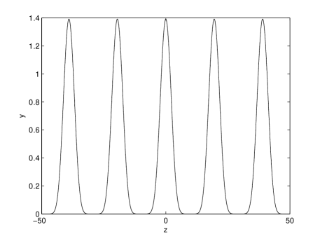
Figure 2: Solution of Eq. (37) in the case $N=4$, $m=2$, $C_{0}=1$, $z_{0}=0$, $\alpha_{0}=1$, $\alpha_{1}=1$.

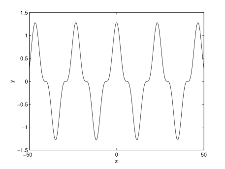
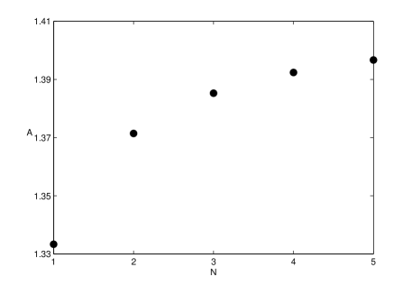
Note, that the amplitude and period of the traveling wave solution are growing with the increasing of $N$. The dependence of amplitude on $N$ is illustrated in Fig. $3$ in the case $m=2$.

Refer to caption
Figure 3: The dependence of amplitude of the traveling wave solution on $N$.

In the general case solution of the family of equations (1) takes the form (4), where parameters $A_{N},B_{N}$ can be written as

$$A_{N}=\frac{2^{N}C_{0}\underset{j=0}{\overset{N-1}{\prod}}((N-j)m+j)}{\alpha_{0}\underset{j=0}{\overset{N-1}{\prod}}((2(N-j)-1)m+2j+1)},$$ (38)
$$B_{N}=\sqrt{\frac{\alpha_{0}}{\alpha_{1}}}\frac{(m-1)P^{N-1}_{N}}{\underset{j=0}{\overset{N-1}{\prod}}((N-j)m+j)},$$ (39)

for mβ‰ βˆ’2​j+12​(Nβˆ’j)βˆ’1π‘š2𝑗12𝑁𝑗1m\neq-\frac{2j+1}{2(N-j)-1}, $-\frac{j}{N-j}$ $(j=0,1,...,N-1)$. $P^{N-1}_{N}$ are polynomials of $N-1$ power. Relations for values of the coefficients $\alpha_{k}$ $(k=0,1,..,N)$ are found from (9).

7 Conclusion

Let us formulate shortly the results of this paper. We have studied the generalized $K(m,m)$ equations. Taking into consideration the traveling wave ansatz we have found the periodic wave solutions for a family of nonlinear partial differential equation (1). This family generalizes a well-known K(m,n) equation in the case $n=m$. Formula for the amplitude of the traveling wave in the general case is given. Exact solutions for the cases $N=1,2,3,4$ of the family (1) are presented.

Acknowledgment

This work was supported by the Federal target programm ”Research and scientific-pedagogical personnel of innovation in Russia” of 2009-2011.

References

  • [1] Rosenau P. and Hyman J., Compactons : Solitons with Finite Wavelength, Phys. Rev. Lett. 1993;5:70.
  • [2] Rosenau P., Nonlinear Dispertion and Compact Structures, Phys. Rev. Lett. 1994;13:73.
  • [3] Rosenau P., On a class of nonlinear dispersive-dissipative interaction, Physica D 1998;123(1-4).
  • [4] Rosenau P., Compact and noncompact dispersive structure. Phys Lett A 2000;275(3):193-203.
  • [5] Tian L.X., Yin J.L., Stability of multi-compacton solutions and Backlund transformation in K(m,n,1). Chaos, Solitons and Fractals 2005;23(1):159-69.
  • [6] Zhu Y., Gao X.S., Exact special solitary solutions with compact support for the nonlinear dispersive K(m, n) equations, Chaos Solitons Fractals 2006;27(2):487-493.
  • [7] Zhu Y.G., Lu Z.S., New exact solitary-wave special solutions for the nonlinear dispersive K(m,n) equations. Chaos, Solitons and Fractals 2006;27(3):836-42.
  • [8] Odibat Z. M., Solitary solutions for the nonlinear dispersive K(m,n) equations with fractional time derivatives, Phys. Lett. A 2007;370:295-301.
  • [9] Xu L., Variational approach to solitons of nonlinear dispersive K(m,n) equations, Chaos, Solitons and Fractals 2008;37:137-143.
  • [10] Biswas A., 1-soliton solution of the K(m,n) equation with generalized evolution, Phys. Lett. A 2008;372(25):4601-4602.
  • [11] Wang D.-S., Lou S. Y., Prolongation structures and exact solutions of K(m,n) equations, J. Math. Phys. 2009;50:123513.
  • [12] M.S. Bruzon, M.L. Gandarias, Traveling wave solutions of the K(m,n) equations with generalized evolution, AIP Conference Proceedings 2009;1168:244-247.
  • [13] Bruzon M.S., Gandarias M.L., Classical potential symmetries of the K(m,n) equation with generalized evolution term, Computers and Mathematics with Applications 2010;59(8):2536-2540.
  • [14] Biswas A., 1-soliton solution of the K(m,n) equation with generalized evolution and time-dependent damping and dispersion, Computers and Mathematics with Applications 2010;59:2536-2540.
  • [15] Kudryashov N.A., Exact soliton solutions of the generalized evolution equation of wave dynamics, J. Appl. Math. Mech. 1988;52(3):360-365.
  • [16] Kudryashov N.A., On types nonlinear nonintegrable differential equations with exact solutions, Phys. Lett. A 1991;155:269-275.
  • [17] Kudryashov N.A., Partial differential equations with solutions having movable forst - order singularities, Physics Letters A 1992;169:237-242.
  • [18] Fu S., Liu S., Liu S., New exact solutions to the KdV Burgers Kuramoto equation, Chaos Solitons Fract. 2005;23:609-616.
  • [19] Kudryashov N.A., Exact solitary waves of the Fisher equation, Phys. Lett. A 2005;342:99-106.
  • [20] Kudryashov N.A., Simplest equation method to look for exact solutions of nonlinear differential equations, Chaos Solitons Fract. 2005;24:1217-1231.
  • [21] Kudryashov N.A., Demina M.V., Polygons of differential equation for finding exact solutions, Chaos Solitons Fract. 2007;33:1480-1496.
  • [22] Kudryashov N.A., Loguinova N.B., Extended simplest equation method for nonlinear differential equations, Appl. Math. Comput. 2008;205(1):396-402.
  • [23] M. Qin, G. Fan, An effective method for finding special solutions of nonlinear differential equations with variable coefficients, Phys. Lett. A 2008;372:3240-3242.
  • [24] Kudryashov N.A., Solitary and periodic solutions of the generalized Kuramoto Sivashinsky equation, Regul. Chaotic Dynam. 2008;13(3):234-238.
  • [25] Lu D., Hong B., Tian L., New solitary wave and periodic wave solutions for general types of KdV and KdV Burgers equations, Commun. Nonlinear Sci. Numer. Simul. 2009;14:77-84.
  • [26] Kudryashov N.A., Loguinova N.B., Be careful with Exp-function method, Commun. Nonlinear Sci. Numer. Simul. 2009;14:1881-1890.
  • [27] Kudryashov N.A., Seven common errors in finding exact solutions of nonlinear differential equations, Commun. Nonlinear Sci. Numer. Simul. 2009;14:3507-3529.
  • [28] Kudryashov N.A., Demina M.V., Traveling wave solutions of the generalized nonlinear evolution equations, Appl. Math. Comput. 2009;210:551-557.
  • [29] Kudryashov N.A., Meromorphic solutions of nonlinear ordinary differential equations, Commun. Nonlinear Sci. Numer. Simul. 2010;15:2778-2790.