Phenomenological aspects of Supersymmetry: SUSY models and electroweak symmetry breaking

These lectures are a very brief introduction to low energy supersymmetry (SUSY). The approach to the construction of SUSY Lagrangians based on the superfield formalism is considered. The minimal supersymmetric standard model (MSSM) is specified. The breakdown of gauge symmetry and Higgs phenomenology within the simplest SUSY extensions of the standard model (SM) are briefly reviewed. The upper bound on the mass of the lightest Higgs boson and little hierarchy problem in SUSY models are discussed.

1 Introduction

As is well known, the Standard Model (SM) describes perfectly the major part of all experimental data measured in earth based experiments. The Lagrangian of the SM is invariant under Poincare group and $SU(3)_{C}\times SU(2)_{W}\times U(1)_{Y}$ gauge symmetry transformations. The Poincare group is an extension of Lorentz group that includes time and space translations

$$|\Psi>\to\exp\{-i\hat{H}t\}|\Psi>,\qquad\qquad|\Psi>\to\exp\{i\hat{\mathbf{P}}\cdot\mathbf{x}\}|\Psi>,$$

where $\hat{H}$ is a Hamiltonian and $\hat{\mathbf{P}}$ are momentum operators.

The transformations of Lorentz group involve rotations about three axes and Lorentz boosts along them. Thus there are three generators of Lorentz group $J_{a}$ which are associated with the rotations around three different axes and there are three other generators $K_{a}$ of this group which correspond to the Lorentz boosts along these axes. Then Lorentz transformations of spin $J$ particle are given by

$$|J>\to\exp\{i\left(J_{a}\theta_{a}+K_{b}\omega_{b}\right)\}|J>,$$

where $\theta_{a}$ are three rotation angles, while $\omega_{b}$ are parameters which are related to the boost velocity $v$. When $\omega_{2}=\omega_{3}=0$ the parameter $\omega_{1}$ is defined as $\mbox{tanh}\,\omega_{1}\,=v$. The commutation relations between the generators of the Lorentz group can be written as

$$\left[J_{a},J_{b}\right]=i\varepsilon_{abc}J_{c}\,,\qquad\left[J_{a},K_{b}\right]=i\varepsilon_{abc}K_{c}\,,\qquad\left[K_{a},K_{b}\right]=-i\varepsilon_{abc}J_{c}\,,$$ (1)

where $a,b,c=1,2,3$.

It is convenient to introduce two linear combinations of the generators of Lorentz group $L_{a}=\frac{1}{2}\left(J_{a}+iK_{a}\right)$ and $N_{a}=\frac{1}{2}\left(J_{a}-iK_{a}\right)$. $L_{a}$ and $N_{a}$ obey two separate $SU(2)$ algebras

$$\left[L_{a},L_{b}\right]=i\varepsilon_{abc}L_{c}\,,\qquad\left[N_{a},N_{b}\right]=i\varepsilon_{abc}N_{c}\,,\qquad\left[L_{a},N_{b}\right]=0\,.$$

As a result the representations of the Lorentz group are classified by two half integer numbers $(j_{1},\,j_{2})$ which are associated with the representations of these two $SU(2)$ algebras. The representations $(j,j)$ correspond to integer spin particles with spin $2j$. The simplest spinor representations are $\psi_{L}=(1/2,\,0)$ and $\psi_{R}=(0,\,1/2)$. The states $\psi_{L}$ and $\psi_{R}$ transform differently under the Lorentz transformations. Indeed, in the fundamental representation $L_{a}=\frac{1}{2}\sigma_{a}$ and $N_{b}=\frac{1}{2}\sigma^{\prime}_{a}$ where $\sigma_{a}$ and $\sigma^{\prime}_{a}$ are $2\times 2$ Pauli matrices. Then in the case of $(1/2,\,0)$ representation $J_{a}=\frac{1}{2}\sigma_{a}$ and $K_{a}=-\frac{i}{2}\sigma_{a}$ so that

$$\Psi_{L}\to\exp\left\{i\frac{\sigma_{a}}{2}\theta_{a}+\frac{\sigma_{b}}{2}\omega_{b}\right\}\Psi_{L}\,.$$ (2)

For $(0,\,1/2)$ representation we have $J_{a}=\frac{1}{2}\sigma^{\prime}_{a}$, $K_{a}=\frac{i}{2}\sigma^{\prime}_{a}$ and

$$\Psi_{R}\to\exp\left\{i\frac{\sigma^{\prime}_{a}}{2}\theta_{a}-\frac{\sigma^{\prime}_{b}}{2}\omega_{b}\right\}\Psi_{R}\,.$$ (3)

Thus from Eqs. (2) and (3) it follows that $\psi_{L}$ and $\psi_{R}$ transform differently under the Lorentz boosts.

Two spinor representations $(1/2,\,0)$ and $(0,\,1/2)$ are called left–handed and right–handed Weyl spinors. The direct sum of the two Weyl spinor states $(1/2,\,0)\oplus(0,\,1/2)$ describes massive spin $1/2$ (Dirac) state

$$\Psi(x)=\left(\begin{array}[]{c}\psi_{\alpha}(x)\\[2.84526pt] \overline{\chi}^{\,\dot{\alpha}}(x)\end{array}\right)\,.$$

In a Weyl representation $\psi_{\alpha}(x)$ and $\overline{\chi}^{\,\dot{\alpha}}(x)$ are associated with $(1/2,\,0)$ and $(0,\,1/2)$ spinor representations, i.e. left–handed and right–handed Weyl spinors. In the case of massless particle $\psi(x)$ and $\overline{\chi}(x)$ have negative and positive helicity. Under parity transformations $\psi(x)\leftrightarrow\overline{\chi}(x)$. Charge conjugation results in

$$\Psi^{C}=C\,\overline{\Psi}^{\small T}=\left(\begin{array}[]{cc}i\sigma_{2}&0\\[2.84526pt] 0&-i\sigma_{2}\end{array}\right)\left(\begin{array}[]{c}\overline{\chi}^{\,\dot{\beta}\,\dagger}\\[2.84526pt] \psi^{\dagger}_{\beta}\end{array}\right)=\left(\begin{array}[]{cc}\varepsilon_{\alpha\beta}&0\\[2.84526pt] 0&\varepsilon^{\dot{\alpha}\dot{\beta}}\end{array}\right)\left(\begin{array}[]{c}\overline{\chi}^{\,\dot{\beta}\,\dagger}\\[2.84526pt] \psi^{\dagger}_{\beta}\end{array}\right)=\left(\begin{array}[]{c}\chi_{\alpha}\\[2.84526pt] \overline{\psi}^{\,\dot{\alpha}}\end{array}\right),$$

where $(i\sigma_{2}\overline{\chi}^{\dagger})_{\alpha}=\chi_{\alpha}$ and $(-i\sigma_{2}\psi^{\dagger})^{\,\dot{\alpha}}=\overline{\psi}^{\,\dot{\alpha}}$. The states $\chi_{\alpha}$ and $\overline{\psi}^{\,\dot{\alpha}}$ transform under Lorentz transformations as $(1/2,\,0)$ and $(0,\,1/2)$. In the Weyl representation the Lagrangian that describes free Dirac fermion with mass $m$ can be written as

$${\cal L}_{D}=i\biggl{(}\chi\sigma^{\mu}\partial_{\mu}\bar{\chi}+\bar{\psi}\bar{\sigma}^{\mu}\partial_{\mu}\psi\biggr{)}-m\biggl{(}\chi\psi+\bar{\psi}\bar{\chi}\biggr{)}\,,$$

where $\sigma^{\mu}=(1,\sigma^{i})$,  $\overline{\sigma}^{\mu}=(1,-\sigma^{i})$ and $\sigma^{i}$ are Pauli matrices. From now on we use abbreviated notations

$$\begin{array}[]{c}\chi\psi=\chi_{\alpha}\varepsilon^{\alpha\beta}\psi_{\beta}=\chi^{\beta}\psi_{\beta}\,,\qquad\qquad\bar{\psi}\bar{\chi}=\bar{\psi}^{\dot{\alpha}}\varepsilon_{\dot{\alpha}\dot{\beta}}\bar{\chi}^{\dot{\beta}}=\bar{\psi}_{\dot{\beta}}\bar{\chi}^{\dot{\beta}}\,,\\[5.69054pt] \chi\sigma^{\mu}\partial_{\mu}\bar{\chi}=\chi^{\alpha}\sigma^{\mu}_{\alpha\dot{\alpha}}\partial_{\mu}\bar{\chi}^{\dot{\alpha}}\,,\qquad\qquad\bar{\psi}\bar{\sigma}^{\mu}\partial_{\mu}\psi=\bar{\psi}_{\dot{\alpha}}(\sigma^{\mu})^{\dot{\alpha}\alpha}\partial_{\mu}\psi_{\alpha}\,.\end{array}$$

A Majorana spinor is defined as one which is equal to its own charge conjugate, i.e. $\Psi^{T}_{M}(x)=\left(\psi_{\alpha}(x),\,\overline{\psi}^{\dot{\alpha}}(x)\right)$ . In the Weyl representation the Lagrangian that describes free Majorana fermion with mass $m$ takes the form

$${\cal L}_{M}=i(\psi\sigma^{\mu}\partial_{\mu}\bar{\psi})-\frac{m}{2}\biggl{(}\psi\psi+\bar{\psi}\bar{\psi}\biggr{)}\,,$$

The six generators of the Lorentz group $J_{a}$ and $K_{a}$ can be presented as antisymmetric tensor $M_{\mu\nu}=-M_{\nu\mu}$. The components of $M_{\mu\nu}$ are $K_{a}=M_{0a}$ and $J_{a}=\frac{1}{2}\varepsilon_{abc}M_{bc}$. $M_{\mu\nu}$ is called angular momentum tensor. The translation operators $\hat{P}_{\mu}=(\hat{H},\hat{P}_{1},\hat{P}_{2},\hat{P}_{3})$ and the angular momentum tensor $M_{\mu\nu}$ form a complete set of generators of the Poincare group which obey algebra

$$\begin{array}[]{c}\left[M_{\mu\nu},M_{\rho\sigma}\right]=i\left(g_{\nu\rho}M_{\mu\sigma}-g_{\mu\rho}M_{\nu\sigma}-g_{\nu\sigma}M_{\mu\rho}+g_{\mu\sigma}M_{\nu\rho}\right)\,,\\[5.69054pt] \left[\hat{P}_{\mu},\,\hat{P}_{\nu}\right]=0\,,\qquad\qquad\left[M_{\mu\nu},\hat{P}_{\lambda}\right]=i\left(g_{\nu\lambda}\hat{P}_{\mu}-g_{\mu\lambda}\hat{P}_{\nu}\right)\,.\end{array}$$ (4)

The generators $T^{a}$ associated with $SU(3)_{C}\times SU(2)_{W}\times U(1)_{Y}$ gauge symmetry (internal symmetry group) commute with the generators of Poincare group. It was established experimentally that $SU(2)_{W}\times U(1)_{Y}$ symmetry is broken. The corresponding massive $W^{\pm}$ and $Z$ bosons were discovered more than 30 years ago. Their properties have been studied in great detail both theoretically and experimentally. Quarks and gluons that participate in the strong interactions are confined inside mesons and baryons and therefore cannot be observed directly. Nevertheless theory of strong interactions based on $SU(3)_{C}$ provides a good description for the spectrum of mesons and baryons, $e^{+}e^{-}$ annihilation data, deep inelastic scattering etc.

Nowadays Higgs boson remains the only missing piece of the SM that has not been discovered yet. It plays a key role in the SM and its extensions. Higgs field acquires vacuum expectation value (VEV) breaking electroweak (EW) symmetry and generating masses of bosons and fermions.

Although the SM describes the major part of experimental data with high accuracy it does not allow to incorporate consistently gravitational interactions. Indeed, in order to achieve the unification of gauge interactions with gravity we need to combine Poincare and internal symmetries. At the same time according to the Coleman-Mandula theorem the most general symmetry which quantum field theory can have is a tensor product of the Poincare group and an internal group [1]. The Coleman-Mandula theorem can be overcome within graded Lie algebras that have the following structure

$$\left[\hat{B},\hat{B}\right]=\hat{B},\qquad\left[\hat{B},\hat{F}\right]=\hat{F},\qquad\left\{\hat{F},\hat{F}\right\}=\hat{B},$$

where $\hat{B}$ and $\hat{F}$ are bosonic and fermionic generators. Graded Lie algebras that contain the Poincare algebra are called supersymmetries. The simplest $N=1$ supersymmetry (SUSY) involves a single Weyl spinor operator $Q_{\alpha}$ and its complex conjugate $Q_{\alpha}^{\dagger}=\overline{Q}_{\,\dot{\alpha}}$. These operators change the spin of the state, i.e.

$$Q_{\alpha}|fermion>=|boson>,\qquad\overline{Q}_{\dot{\alpha}}|boson>=|fermion>.$$

The $N=1$ SUSY algebra is Poincare algebra (4) plus

$$\begin{array}[]{ll}\left\{Q_{\alpha},\overline{Q}_{\dot{\alpha}}\right\}=2\,\sigma^{\mu}_{\alpha\dot{\alpha}}\hat{P}_{\mu},&\left\{Q_{\alpha},Q_{\beta}\right\}=\left\{\overline{Q}_{\dot{\alpha}},\overline{Q}_{\dot{\alpha}}\right\}=0,\\[5.69054pt] \left[\hat{P}_{\mu},Q_{\alpha}\right]=0,&\left[M^{\mu\nu},Q_{\alpha}\right]=-i\left(\sigma^{\mu\nu}\right)^{\beta}_{\alpha}Q_{\beta},\\[5.69054pt] \left[\hat{P}^{\mu},\overline{Q}_{\dot{\alpha}}\right]=0,&\left[M^{\mu\nu},\overline{Q}^{\dot{\alpha}}\right]=-i\left(\sigma^{\mu\nu}\right)^{\dot{\alpha}}_{\dot{\beta}}\overline{Q}^{\dot{\beta}},\end{array}$$ (5)

where $\sigma^{\mu\nu}=\frac{1}{4}\left(\sigma^{\mu}\overline{\sigma}^{\nu}-\sigma^{\nu}\overline{\sigma}^{\mu}\right)$, and $\overline{\sigma}^{\mu\nu}=\frac{1}{4}\left(\overline{\sigma}^{\mu}\sigma^{\nu}-\overline{\sigma}^{\nu}\sigma^{\mu}\right)$. The local version of SUSY (supergravity) leads to a partial unification of gauge interactions with gravity [2]-[4].

This course of lectures is a very basic introduction to $N=1$ supersymmetry. In section 2 chiral and vector superfields are introduced. In section 3 these superfields are used for the construction of SUSY Lagrangians. The minimal supersymmetric standard model (MSSM) is specified in section 4. In section 5 the breakdown of gauge symmetry and Higgs phenomenology within the simplest SUSY extensions of the SM are considered.

Nowadays there are many excellent books [5]–[10], introductions [11]–[25] and reviews [26]–[29] of supersymmetry available while in this paper only a few aspects of SUSY are briefly discussed. Students and early–career researchers, who got really interested in supersymmetry, should definitely study some of the books, reviews and/or introductions mentioned in the list of references of this lecture notes.

2 Superspace and superfields

An elegant formulation of supersymmetry transformations and invariants can be achieved in the framework of superspace. Superspace differs from the ordinary Euclidean (Minkowski) space by adding of new fermionic coordinates, $\theta_{\alpha}$ and $\bar{\theta}_{\dot{\alpha}}$, that change in a certain way under the enlarged group of transformations. These new coordinates are anticommuting Grassmann variables transforming as two–component Weyl spinors:

$$\{\theta_{\alpha},\theta_{\beta}\}=0\,,\qquad\{\bar{\theta}_{\dot{\alpha}},\bar{\theta}_{\dot{\beta}}\}=0\,,\qquad\theta_{\alpha}^{2}=0\,,\qquad\bar{\theta}_{\dot{\alpha}}^{2}=0\,,$$

where $\alpha,\,\beta,\,\dot{\alpha},\,\dot{\beta}=1,2$. Fermionic coordinates arise in a SUSY transformation that can be constructed in superspace in the same way as an ordinary translation in the usual space

$$G(x,\theta,\bar{\theta})=e^{\displaystyle i(-x^{\mu}P_{\mu}+\theta Q+\bar{\theta}\bar{Q})}.$$ (6)

Using the Hausdorff formula

$$e^{A}e^{B}=\exp(A+B+\frac{1}{2}[A,B]+...)\,,$$

that terminates at the first commutator for the group elements considered here, one can combine two SUSY transformations

$$G(x^{\mu},\theta,\bar{\theta})G(a^{\mu},\xi,\bar{\xi})=G(x^{\mu}+a^{\mu}-i\xi\sigma^{\mu}\bar{\theta}+i\theta\sigma^{\mu}\bar{\xi},\theta+\xi,\bar{\theta}+\bar{\xi})\,.$$ (7)

This leads to a supertranslation in superspace

$$\begin{array}[]{ccl}x_{\mu}&\rightarrow&x_{\mu}+a_{\mu}+i\theta\sigma_{\mu}\bar{\xi}-i\xi\sigma_{\mu}\bar{\theta}\,,\\[5.69054pt] \theta&\rightarrow&\theta+\xi\,,\\[5.69054pt] \bar{\theta}&\rightarrow&\bar{\theta}+\bar{\xi}\,,\end{array}$$ (8)

where $\xi$ and $\bar{\xi}$ play a role of Grassmannian transformation parameters. Taking these parameters to be local, or space-time dependent, one gets a local translations that result in a theory of (super) gravity.

Whereas an ordinary field is a function of the space–time coordinates $x$ only, a superfield $S(x,\theta,\bar{\theta})$ is also a function of anticommuting Grassmann variables $\theta_{\alpha}$ and $\bar{\theta}_{\dot{\alpha}}$. The fields of the supermultiplet then arise as the coefficients in an expansion of $S(x,\theta,\bar{\theta})$ in powers of $\theta_{\alpha}$ and $\bar{\theta}_{\dot{\alpha}}$. Assuming that $a_{\mu}$, $\xi$ and $\bar{\xi}$ are infinitesimally small we can Taylor expand $S(x^{\prime\mu},\theta^{\prime},\bar{\theta}^{\prime})$

$$\begin{array}[]{c}S(x^{\mu}+a^{\mu}-i\xi\sigma^{\mu}\bar{\theta}+i\theta\sigma^{\mu}\bar{\xi},\theta+\xi,\bar{\theta}+\bar{\xi})\simeq S(x^{\mu},\theta,\bar{\theta})+\\[5.69054pt] \displaystyle(a^{\mu}-i\xi\sigma^{\mu}\bar{\theta}+i\theta\sigma^{\mu}\bar{\xi})\frac{\partial S}{\partial x^{\mu}}+\xi^{\alpha}\frac{\partial S}{\partial\theta^{\alpha}}+\bar{\xi}_{\dot{\alpha}}\frac{\partial}{\bar{\theta}_{\dot{\alpha}}}+...\end{array}$$ (9)

By comparing the coefficients of the infinitesimal parameters $a_{\mu}$, $\xi$ and $\bar{\xi}$ one can see that the action of the SUSY algebra on superfields

$$S(x^{\mu},\theta,\bar{\theta})\rightarrow e^{\displaystyle i(-a^{\mu}P_{\mu}+\xi Q+\bar{\xi}\bar{Q})}S(x^{\mu},\theta,\bar{\theta})$$ (10)

is generated by

$$P_{\mu}=i\partial_{\mu},\qquad iQ_{\alpha}=\frac{\partial}{\partial\theta^{\alpha}}-i\sigma^{\mu}_{\alpha\dot{\alpha}}\bar{\theta}^{\dot{\alpha}}\partial_{\mu}\,,\qquad i\bar{Q}_{\dot{\alpha}}=-\frac{\partial}{\partial\bar{\theta}^{\dot{\alpha}}}+i\theta^{\alpha}\sigma^{\mu}_{\alpha\dot{\alpha}}\partial_{\mu}.$$ (11)

The general superfield $S(x^{\mu},\theta,\bar{\theta})$ can be expanded as a power series in $\theta_{\alpha}$ and $\bar{\theta}_{\dot{\alpha}}$ involving not more than two powers of $\theta_{\alpha}$ and $\bar{\theta}_{\dot{\alpha}}$ since $\theta_{\alpha}$ and $\bar{\theta}_{\dot{\alpha}}$ are two–component Grassmann variables. Scalar superfield $S(x^{\mu},\theta,\bar{\theta})$ is the simplest representation of the Super-Poincare group. However such superfield is a reducible representation of SUSY. Irreducible representations of the SUSY algebra are obtained by imposing constraints which are covariant under the supersymmetry algebra.

In this context it is convenient to define fermionic derivatives

$$D_{\alpha}=\displaystyle\frac{\partial}{\partial\theta^{\alpha}}+i\sigma^{\mu}_{\alpha\dot{\alpha}}\bar{\theta}^{\dot{\alpha}}\partial_{\mu}\,,\qquad\bar{D}_{\dot{\alpha}}=\displaystyle-\frac{\partial}{\partial\bar{\theta}^{\dot{\alpha}}}-i\theta^{\alpha}\sigma^{\mu}_{\alpha\dot{\alpha}}\partial_{\mu}\,.$$ (12)

The derivatives $D_{\alpha}$ and $\bar{D}_{\dot{\alpha}}$ anticommute with the generators of the SUSY algebra, i.e.

$$\{D_{\alpha},Q_{\beta}\}=\{D_{\alpha},\bar{Q}_{\dot{\beta}}\}=\{\bar{D}_{\dot{\alpha}},Q_{\beta}\}=\{\bar{D}_{\dot{\alpha}},\bar{Q}_{\dot{\beta}}\}=0\,.$$ (13)

On the other hand they obey algebra

$$\{D_{\alpha},\bar{D}_{\dot{\alpha}}\}=2i\sigma^{\mu}_{\alpha\dot{\alpha}}\partial_{\mu}\,,\qquad\{D_{\alpha},D_{\beta}\}=\{\bar{D}_{\dot{\alpha}},\bar{D}_{\dot{\beta}}\}=0\,.$$ (14)

The superspace covariant derivatives $D_{\alpha}$ and $\bar{D}_{\dot{\alpha}}$ can be used to impose covariant constraints on superfields because they commute with $\xi Q+\bar{\xi}\bar{Q}$ which occurs in SUSY transformations (10). Indeed, if superfield $\Phi(x^{\mu},\theta,\bar{\theta})$ satisfies the covariant condition

$$\bar{D}_{\dot{\alpha}}\Phi(x^{\mu},\theta,\bar{\theta})=0\,,$$ (15)

then after SUSY transformation the corresponding superfield still satisfies constraint (15). Superfield $\Phi(x^{\mu},\theta,\bar{\theta})$ which obey condition (15) is called a chiral superfield.

It is worth to point out that

$$\bar{D}_{\dot{\alpha}}\theta_{\alpha}=0\,,\qquad\bar{D}_{\dot{\alpha}}y^{\mu}=0\,,$$ (16)

where $y^{\mu}=x^{\mu}+i\theta\sigma^{\mu}\bar{\theta}$. Thus any function of $\theta$ and $y^{\mu}$ satisfies the covariant condition (15). Expanding $\Phi(y^{\mu},\theta)$ in powers of the two-component Grassmann variable $\theta$ gives

$$\Phi(y,\theta)=\phi(y)+\sqrt{2}\,\theta\psi(y)+\theta\theta F(y)\,,$$ (17)

where $\phi$ is a complex scalar field, $F$ is an auxiliary complex scalar field and $\psi$ is a left–handed Weyl spinor field. The coefficients in expansion (17) are called the components of a superfield. The general expansion of chiral superfield (17) in component fields around $x^{\mu}$ is

$$\begin{array}[]{c}\displaystyle\Phi(x^{\mu},\theta,\bar{\theta})=\phi(x)+\sqrt{2}\,\theta\psi(x)+(\theta\theta)F(x)+i(\theta\sigma^{\mu}\bar{\theta})\partial_{\mu}\phi(x)\\[5.69054pt] \displaystyle-\frac{i}{\sqrt{2}}(\theta\theta)(\partial_{\mu}\psi(x)\sigma^{\mu}\bar{\theta})-\frac{1}{4}(\theta\theta)(\bar{\theta}\bar{\theta})\partial_{\mu}\partial^{\mu}\phi(x)\,.\end{array}$$ (18)

The fields $\phi(x)$ and $\psi(x)$ are called superpartners. From expansion (17) it follows that chiral superfield has the same number of bosonic and fermionic degrees of freedom. The mass dimensions of scalars and spinors in Eq. (17) are $[\phi]=1$, $[\psi]=3/2$, $[F]=2$ and $[\theta]=-1/2$ whereas chiral superfield has mass dimension 1, i.e. $[\Phi]=1$

One can also construct an antichiral (conjugate) superfield $\Phi^{\dagger}(x^{\mu},\theta,\bar{\theta})$ that has the component field expansion

$$\begin{array}[]{c}\displaystyle\Phi^{\dagger}(x^{\mu},\theta,\bar{\theta})=\phi^{\dagger}(x)+\sqrt{2}\,\bar{\theta}\bar{\psi}(x)+(\bar{\theta}\bar{\theta})F^{\dagger}(x)-i(\theta\sigma^{\mu}\bar{\theta})\partial_{\mu}\phi^{\dagger}(x)\\[5.69054pt] \displaystyle+\frac{i}{\sqrt{2}}(\bar{\theta}\bar{\theta})(\theta\sigma^{\mu}\partial_{\mu}\bar{\psi}(x))-\frac{1}{4}(\theta\theta)(\bar{\theta}\bar{\theta})\partial_{\mu}\partial^{\mu}\phi^{\dagger}(x)\,.\end{array}$$ (19)

This superfield obey equation

$$D_{\alpha}\Phi^{\dagger}(x^{\mu},\theta,\bar{\theta})=0\,.$$ (20)

Since $\Phi(x^{\mu},\theta,\bar{\theta})$ involves left–handed Weyl spinor $\psi$ while $\Phi^{\dagger}(x^{\mu},\theta,\bar{\theta})$ contains right–handed Weyl spinor $\bar{\psi}$, $\Phi(x^{\mu},\theta,\bar{\theta})$ and $\Phi^{\dagger}(x^{\mu},\theta,\bar{\theta})$ are sometimes called left–handed and right–handed chiral superfields.

The SUSY transformation of chiral superfield (10) induces transformations of its components. Under an infinitesimal SUSY transformation the left–handed superfield changes as follows

$$\begin{array}[]{l}\Phi\rightarrow\Phi+\delta\Phi\,,\\[5.69054pt] \delta\Phi=i(\xi Q+\bar{\xi}\bar{Q})\Phi=\delta\phi(x)+\sqrt{2}\,\theta\delta\psi(x)+(\theta\theta)\delta F(x)+...\end{array}$$ (21)

Using the explicit expressions for $Q$ and $\bar{Q}$ (see Eq. (11)), we find

$$\delta\phi = \sqrt{2}\,\xi\psi\,,$$

$$\delta\psi = i\sqrt{2}\,\sigma^{\mu}\bar{\xi}\partial_{\mu}\phi+\sqrt{2}\,\xi F\,,$$ (22)

$$\delta F = i\sqrt{2}\,\partial_{\mu}\psi\sigma^{\mu}\bar{\xi}\,.$$

As expected the change in the bosonic (fermionic) component of the superfield is proportional to the fermionic (bosonic) fields. It is important to notice that the change in $F$ component under a SUSY transformation is a total derivative. Therefore this component of chiral superfield can be used for the construction of SUSY Lagrangians

For the construction of SUSY Lagrangians it is also necessary to study the products of chiral superfields and $\Phi^{\dagger}_{i}\Phi_{j}$. Because $Q_{\alpha}$, $\bar{Q}_{\dot{\alpha}}$ and covariant derivatives $D_{\alpha}$ and $\bar{D}_{\dot{\alpha}}$ are linear differential operators on superspace any product of chiral (antichiral) superfields $\Phi_{i}\Phi_{j}$, $\Phi_{i}\Phi_{j}\Phi_{k}$ etc is again a chiral (antichiral) superfield so that the covariant condition (15) is fulfilled. Direct calculation gives

$$\begin{array}[]{c}\Phi_{i}(y,\theta)\Phi_{j}(y,\theta)=\phi_{i}(y)\phi_{j}(y)+\sqrt{2}\,\theta(\psi_{i}(y)\phi_{j}(y)+\phi_{i}(y)\psi_{j}(y))\\[5.69054pt] +(\theta\theta)(\phi_{i}(y)F_{j}(y)+\phi_{j}(y)F_{i}(y)-\psi_{i}(y)\psi_{j}(y))\,,\end{array}$$ (23)

$$\begin{array}[]{c}\Phi_{i}(y,\theta)\Phi_{j}(y,\theta)\Phi_{k}(y,\theta)=\phi_{i}(y)\phi_{j}(y)\phi_{k}(y)+\sqrt{2}\,\theta(\psi_{i}(y)\phi_{j}(y)\phi_{k}(y)+\\[5.69054pt] \phi_{i}(y)\psi_{j}(y)\phi_{k}(y)+\phi_{i}(y)\phi_{j}(y)\psi_{k}(y))+(\theta\theta)(\phi_{i}(y)\phi_{j}(y)F_{k}(y)+\\[5.69054pt] \phi_{i}(y)F_{j}(y)\phi_{k}(y)+F_{i}(y)\phi_{j}(y)\phi_{k}(y)-\psi_{i}(y)\psi_{j}(y)\phi_{k}(y)\\[5.69054pt] -\psi_{i}(y)\psi_{k}(y)\phi_{j}(y)-\psi_{j}(y)\psi_{k}(y)\phi_{i}(y))\,,\end{array}$$ (24)

For any arbitrary function of chiral superfields one gets

$$W(\Phi_{k}) = W(\phi_{k}+\sqrt{2}\theta\psi_{k}+\theta\theta F_{k})=W(\phi_{k})+\frac{\partial W(\phi_{k})}{\partial\phi_{i}}\sqrt{2}\theta\psi_{i}$$ (25)

$$+ \theta\theta\left(\frac{\partial W(\phi_{k})}{\partial\phi_{i}}F_{i}-\frac{1}{2}\frac{\partial^{2}W(\phi_{k})}{\partial\phi_{i}\partial\phi_{j}}\psi_{i}\psi_{j}\right).$$

On the other hand the product of the left–handed and right–handed chiral superfields is not a chiral superfield since

$$\begin{array}[]{rcl}\tilde{V}&=&\Phi^{\dagger}_{i}(y,\theta)\Phi_{j}(y,\theta)=\phi^{\dagger}_{i}(y)\phi_{j}(y)+\sqrt{2}\,(\theta\psi_{j}(y))\phi^{\dagger}_{i}(y)+\\[5.69054pt] &&\sqrt{2}\,(\bar{\theta}\bar{\psi}_{i}(y))\phi_{j}(y)+2(\bar{\theta}\bar{\psi}_{i}(y))(\theta\psi_{j}(y))+F_{j}(y)\phi^{\dagger}_{i}(y)(\theta\theta)+\\[5.69054pt] &&F^{\dagger}_{i}(y)\phi_{j}(y)(\bar{\theta}\bar{\theta})+\sqrt{2}\,(\theta\theta)(\bar{\theta}\bar{\psi}_{i}(y))F_{j}(y)+\\[5.69054pt] &&\sqrt{2}\,(\bar{\theta}\bar{\theta})(\theta\psi_{j}(y))F^{\dagger}_{i}(y)+(\bar{\theta}\bar{\theta})(\theta\theta)F^{\dagger}_{i}(y)F_{j}(y)\end{array}$$ (26)

$\tilde{V}$ can not be reduced to the form (17). At the same time the superfield $\tilde{V}(x^{\mu},\theta,\bar{\theta})$ satisfies the constraint

$$\tilde{V}(x^{\mu},\theta,\bar{\theta})=\tilde{V}^{\dagger}(x^{\mu},\theta,\bar{\theta})\,,$$ (27)

which is preserved under SUSY transformations. The superfields that obey condition (27) are called vector superfields. Note that $(\bar{\theta}\bar{\theta})(\theta\theta)$ component of $\tilde{V}(x^{\mu},\theta,\bar{\theta})$ is proportional to $F^{\dagger}_{i}F_{j}$. This is an indication that the coefficient of the $(\bar{\theta}\bar{\theta})(\theta\theta)$ term is a new auxiliary field. This auxiliary field is called $D$. One can anticipate that the new auxiliary field can be also useful in constructing SUSY Lagrangians. After substituting for $y$ we find that

$$\begin{array}[]{c}\displaystyle\left[\Phi^{\dagger}_{i}\Phi_{j}\right]_{D}=F^{\dagger}_{i}F_{j}+\frac{1}{2}\partial_{\mu}\phi^{\dagger}_{i}\partial^{\mu}\phi_{j}-\frac{1}{4}\phi_{i}^{\dagger}\partial_{\mu}\partial^{\mu}\phi_{j}-\frac{1}{4}(\partial_{\mu}\partial^{\mu}\phi_{i}^{\dagger})\phi_{j}\\[5.69054pt] \displaystyle+\frac{i}{2}\bar{\psi}_{i}\bar{\sigma}^{\mu}\partial_{\mu}\psi_{j}-\frac{i}{2}(\partial_{\mu}\bar{\psi}_{i})\bar{\sigma}^{\mu}\psi_{j}\,.\end{array}$$ (28)

Another example of vector superfield that can be constructed using left–handed and right–handed chiral superfields is

$$\begin{array}[]{rcl}V^{\prime}(x,\theta,\bar{\theta})&=&i(\Phi-\Phi^{\dagger})=i(\phi(x)-\phi^{\dagger}(x))+i\sqrt{2}(\theta\psi(x)-\bar{\theta}\bar{\psi}(x))\\[5.69054pt] &&\displaystyle+i(\theta\theta F(x)-\bar{\theta}\bar{\theta}F^{\dagger}(x))-(\theta\sigma^{\mu}\bar{\theta})\partial_{\mu}(\phi(x)+\phi^{\dagger}(x))\\[5.69054pt] &&\displaystyle-\frac{1}{\sqrt{2}}(\theta\theta)(\bar{\theta}\bar{\sigma}^{\mu}\partial_{\mu}\psi(x))+\frac{1}{\sqrt{2}}(\bar{\theta}\bar{\theta})(\theta\sigma^{\mu}\partial_{\mu}\bar{\psi}(x))\\[8.53581pt] &&\displaystyle-\frac{i}{4}(\theta\theta)(\bar{\theta}\bar{\theta})\partial_{\mu}\partial^{\mu}(\phi(x)-\phi^{\dagger}(x))\,.\end{array}$$ (29)

We will use the explicit expression for vector superfield $V^{\prime}(x,\theta,\bar{\theta})$ when we consider (super) gauge transformations.

Without loss of generality any Lorentz invariant superfield may be written in the form

$$\begin{array}[]{c}F(x,\theta,\bar{\theta})=f(x)+\theta\chi^{\prime}(x)+\bar{\theta}\bar{\chi}+\theta\theta m(x)+\bar{\theta}\bar{\theta}\tilde{m}(x)+(\theta\sigma^{\mu}\bar{\theta})V_{\mu}(x)\\[5.69054pt] +\theta\theta\bar{\theta}\bar{\lambda}(x)+\bar{\theta}\bar{\theta}\theta\lambda^{\prime}(x)+\theta\theta\bar{\theta}\bar{\theta}d(x)\,,\end{array}$$ (30)

where $f(x),\,m(x),\,\tilde{m}(x),\,d(x)$ are scalar fields, $V_{\mu}(x)$ is a vector field, and $\chi^{\prime}(x),\,\chi(x),\,\lambda(x),\,\lambda^{\prime}(x)$ are Weyl spinor fields. Because all these fields can be complex the superfield $F(x,\theta,\bar{\theta})$ involves eight complex bosonic and fermionic degrees of freedom. If we require that $F(x,\theta,\bar{\theta})$ is real, i.e. it satisfies condition (27), then

$$\begin{array}[]{c}f(x)=f^{\dagger}(x)\,,\quad m(x)=\tilde{m}^{\dagger}(x)\,,\quad d(x)=d^{\dagger}(x)\,,\quad V_{\mu}(x)=V^{\dagger}_{\mu}(x)\,,\\[5.69054pt] \chi^{\prime}(x)=\chi(x)\,,\quad\lambda(x)=\lambda^{\prime}(x)\,.\end{array}$$ (31)

Thus, through the constraint (27) the eight complex bosonic and fermionic degrees of freedom in Eq. (30) are reduced to eight real bosonic and fermionic degrees of freedom. From Eqs. (30)–(31) it becomes clear that vector superfield contains a real vector field which can play a role of gauge vector boson. Therefore this superfield has to be used to formulate a supersymmetric version of quantum electrodynamics (QED), for example, which involves photon.

It is convenient to rewrite vector superfield using special field combinations for the coefficients of the $\theta\theta\bar{\theta}$, $\bar{\theta}\bar{\theta}\theta$ and $\theta\theta\bar{\theta}\bar{\theta}$ components, i.e.

$$V(x,\theta,\bar{\theta}) = C(x)+i\theta\chi(x)-i\bar{\theta}\bar{\chi}(x)+\frac{i}{2}\theta\theta[M(x)+iN(x)]$$

$$-\frac{i}{2}\bar{\theta}\bar{\theta}[M(x)-iN(x)]-\theta\sigma^{\mu}\bar{\theta}V_{\mu}(x)$$

$$+i\theta\theta\bar{\theta}\biggr{[}\bar{\lambda}(x)+\frac{i}{2}\bar{\sigma}^{\mu}\partial_{\mu}\chi(x)\biggl{]}-i\bar{\theta}\bar{\theta}\theta\biggr{[}\lambda(x)+\frac{i}{2}\sigma^{\mu}\partial_{\mu}\bar{\chi}(x)\biggl{]}$$

$$+\frac{1}{2}\theta\theta\bar{\theta}\bar{\theta}\biggr{[}D(x)-\frac{1}{2}\partial_{\mu}\partial^{\mu}C(x)\biggl{]}\,,$$

where $C(x)$, $M(x)$, $N(x)$, $D(x)$ are real scalar fields. As before, $\chi$ and $\lambda$ are Weyl spinor fields and $V_{\mu}$ is a real vector field. The dimensions of all these fields are fixed by requiring that the vector field $V_{\mu}$ has its canonical mass dimension $[V]=1$. Then

$$[C]=0\,,\quad[\chi]=\frac{1}{2}\,,\quad[M]=[N]=1\,,\quad[\lambda]=\frac{3}{2}\,,\quad[D]=2\,,$$ (33)

while the vector superfield is dimensionless.

In the QED Lagrangian does not change when $V_{\mu}\rightarrow V_{\mu}-\partial_{\mu}\omega$. In SUSY QED $V_{\mu}$ and $\omega$ have to be the appropriate components of SUSY multiplets. Therefore gauge transformation should be defined in terms of superfields. One can expect that $\omega$ might appear as a component of the linear superposition of the left–handed and right–handed chiral superfields that transform as a vector superfield with respect to SUSY transformations. One combination of $\Phi(x,\theta,\bar{\theta})$ and $\Phi^{\dagger}(x,\theta,\bar{\theta})$ that satisfies this requirement was mentioned before (see Eq. (29)). Indeed, if under $U(1)$ gauge transformation $V(x,\theta,\bar{\theta})$ transforms as

$$V(x,\theta,\bar{\theta})\rightarrow V(x,\theta,\bar{\theta})+i\biggl{[}\Phi(x,\theta,\bar{\theta})-\Phi^{\dagger}(x,\theta,\bar{\theta})\biggr{]}\,,$$ (34)

then the components of vector superfield changes as follows

$$C(x) \rightarrow C(x)+i(\phi(x)-\phi^{\dagger}(x))\,,$$

$$\chi(x) \rightarrow \chi(x)+\sqrt{2}\psi(x)\,,$$

$$M(x)+iN(x) \rightarrow M(x)+iN(x)+2F(x)\,,$$

$$V_{\mu}(x) \rightarrow V_{\mu}(x)-\partial_{\mu}(\phi(x)+\phi^{\dagger}(x))\,,$$ (35)

$$\lambda(x) \rightarrow \lambda(x)\,,\qquad D(x)\rightarrow D(x)\,.$$

From Eq. (35) it is easy to see that local $U(1)$ gauge field transforms as in the QED. Thus Eq. (34) can be considered as a supersymmetric generalization of gauge transformation in SUSY QED. One can also see that $C(x)$, $M(x)$, $N(x)$ and $\chi(x)$ are not physical degrees of freedom, since they can be gauged away by a suitable choice of $(\phi(x)-\phi^{\dagger}(x))$, $\psi(x)$ and $F(x)$ while still leaving $\omega(x)=(\phi(x)+\phi^{\dagger}(x))$ arbitrary. In this Wess-Zumino gauge [30] vector superfield takes the form

$$V(x,\theta,\bar{\theta})=-\theta\sigma^{\mu}\bar{\theta}V_{\mu}(x)+i\theta\theta\bar{\theta}\bar{\lambda}(x)-i\bar{\theta}\bar{\theta}\theta\lambda(x)+\frac{1}{2}\theta\theta\bar{\theta}\bar{\theta}D(x)\,.$$ (36)

From (35) it becomes clear that the fields $\lambda(x)$ and $D(x)$ are gauge invariant whereas $V_{\mu}(x)$ transforms as in the usual QED. So $V_{\mu}(x)$ should be associated with the gauge field (photon) while $\lambda(x)$ is called gaugino (photino in SUSY QED). All powers $V^{n}(x,\theta,\bar{\theta})$ with $n>2$ vanish in the Wess-Zumino gauge, since they will involve at least $\theta^{3}$. The only non–zero power is

$$V^{2}(x,\theta,\bar{\theta})=\frac{1}{2}\theta\theta\bar{\theta}\bar{\theta}V_{\mu}(x)V^{\mu}(x)\,.$$

As we have done for the chiral superfield we can now determine the transformation properties of the component fields of $V(x,\theta,\bar{\theta})$. Under an infinitesimal SUSY transformation the vector superfield changes as follows

$$V\rightarrow V+\delta V\,,\qquad\delta V=i(\xi Q+\bar{\xi}\bar{Q})V.$$ (37)

With $Q$ and $\bar{Q}$ given by Eq. (11) we find

$$\delta\lambda_{\alpha} = -iD\xi_{\alpha}-\frac{1}{2}(\sigma^{\mu}\bar{\sigma}^{\nu})^{\beta}_{\alpha}\xi_{\beta}V_{\mu\nu}\,,$$

$$\delta V^{\mu} = i(\xi\sigma^{\mu}\bar{\lambda}-\lambda\sigma^{\mu}\bar{\xi})-\partial^{\mu}(\xi\chi+\bar{\xi}\bar{\chi})\,,$$ (38)

$$\delta D = \partial_{\mu}(-\xi\sigma^{\mu}\bar{\lambda}+\lambda\sigma^{\mu}\bar{\xi})\,,$$

where $V_{\mu\nu}=\partial_{\mu}V_{\nu}-\partial_{\nu}V_{\mu}$. Eqs. (38) lead to the following transformation property of the $U(1)$ field strength $V_{\mu\nu}$

$$\delta V^{\mu\nu}=i\partial^{\mu}(\xi\sigma^{\nu}\bar{\lambda}-\lambda\sigma^{\nu}\bar{\xi})-i\partial^{\nu}(\xi\sigma^{\mu}\bar{\lambda}-\lambda\sigma^{\mu}\bar{\xi}),$$ (39)

that does not depend on the Wel spinor $\chi$. Eqs. (38)–(39) imply that fields $V_{\mu\nu}$, $\lambda$ and $D$ form an irreducible representation of the SUSY algebra by themselves. Note that the variation of the $D$–field is a total divergence as in the case of $F$–field. Since total divergences vanish when integrated over the space time the $F$–components of chiral superfields and the $D$–components of vector superfields can be used to construct SUSY Lagrangians.

3 SUSY Lagrangians

The discussion at the end of the previous section suggests an immediate way to construct Lagrangians which are invariant under SUSY transformations. In the superfield notation SUSY invariant Lagrangians are the polynomials of superfields. Then the key observation for the construction of SUSY theories is that the $F$–term of a chiral superfield (i.e. the $\theta\theta$ component of a left–handed chiral superfield and the $\bar{\theta}\bar{\theta}$ component of a right–handed chiral superfield) and the $D$–term of a vector superfield (i.e. the $\theta\theta\bar{\theta}\bar{\theta}$ component) transform into themselves plus a total derivative under SUSY transformations. Since the action does not change when Lagrangian ${\cal L}$ changes by a total derivative, the SUSY invariant Lagrangian can be written as

$${\cal L}={\cal L}_{D}+{\cal L}_{F}\,,$$ (40)

where ${\cal L}_{F}$ is made up of $F$–terms and ${\cal L}_{D}$ is made up of $D$–terms.

3.1 Lagrangians for chiral superfields

Let us start with the Lagrangian which contains only a set of chiral superfields and has no vector supermultiplets (Wess–Zumino model). Then the most general renormalizable SUSY invariant Lagrangian has the form

$${\cal L}_{WZ}={\cal L}_{D}+{\cal L}_{F}=\sum_{i}\biggl{[}\Phi_{i}^{\dagger}\Phi_{i}\biggr{]}_{D}+\biggl{(}[W(\Phi_{k})]_{F}+h.c.\biggr{)}\,,$$ (41)

where $W(\Phi_{k})$, which is referred to as the superpotential, must involve only up to the third power of the superfields $\Phi_{k}$ to obtain a renormalizable Lagrangian, i.e.

$$W(\Phi_{k})=a_{i}\Phi_{i}+\frac{1}{2}\mu_{ij}\Phi_{i}\Phi_{j}+\frac{1}{3}y_{ijk}\Phi_{i}\Phi_{j}\Phi_{k}\,.$$ (42)

In Eq. (42) the sum over all possible combinations of chiral superfields is understood while $a_{i}$, $\mu_{ij}$ and $y_{ijk}$ are constants. One might think that we could add more terms with products of more than three chiral superfields in the superpotential. In this context it is worth to note that $[\Phi_{i}]_{F}$, $[\Phi_{i}\Phi_{j}]_{F}$ and $[\Phi_{i}\Phi_{j}\Phi_{k}]_{F}$ have mass dimensions 2, 3 and 4 respectively. As a consequence the mass dimensions of various couplings in Eq. (42) are $[a_{i}]=2$, $[\mu_{ij}]=1$ and $[y_{ijk}]=0$ to ensure $[{\cal L}_{F}]=4$. It is obvious that $F$–terms involving more factors of $\Phi_{i}$ will have mass dimension greater than four resulting in couplings with negative mass dimension. The presence of such couplings makes SUSY theory non–renormalizable.

The superpotential $W(\Phi_{k})$ must contain the products of chiral superfields only. In other words $W(\Phi_{k})$ has to be a holomorphic (analytic) function of $\Phi_{k}$. The presence of terms like $\Phi_{i}\Phi^{\dagger}_{j}$, $\Phi_{i}\Phi_{j}\Phi^{\dagger}_{k}$ etc in the superpotential give rise to extra components of superfields that do not appear in the expansion of chiral superfield. Thus $\theta\theta$ component of the superpotential would not transform into itself plus a total derivative and thereby would break SUSY.

As follows from Eq. (28) the first term in Eq. (41) leads to the usual kinetic terms for the components of chiral superfields and $F^{\dagger}_{i}F_{i}$. The term $[\Phi_{i}^{\dagger}\Phi_{i}]_{D}$ has mass dimension 4. Thereby high products of left–handed and right–handed chiral superfields such as $\Phi_{i}\Phi_{j}\Phi^{\dagger}_{k}$, $\Phi_{i}\Phi_{j}\Phi^{\dagger}_{k}\Phi^{\dagger}_{l}$ etc would result in couplings with negative mass dimension, i.e. non–renormalizable interactions. Superpotential in Eq. (41) gives rise to mass terms, Yukawa couplings and scalar potential. Combining Eqs. (28) and (25) one obtains an explicit expression for the most general renormalizable SUSY invariant Lagrangian in the Wess–Zumino model

$${\cal L}_{WZ}=\partial_{\mu}\phi^{\dagger}_{i}\partial^{\mu}\phi_{i}+i\bar{\psi}_{i}\bar{\sigma}^{\mu}\partial_{\mu}\psi_{i}+F^{\dagger}_{i}F_{i}\qquad\qquad\qquad$$

$$\qquad\qquad\qquad+\left(\frac{\partial W(\phi_{k})}{\partial\phi_{i}}F_{i}-\frac{1}{2}\frac{\partial^{2}W(\phi_{k})}{\partial\phi_{i}\partial\phi_{j}}\psi_{i}\psi_{j}+h.c.\right).$$ (43)

Note that in the Lagrangian (43) there is no any kinetic terms for the fields $F_{i}$. This means that the equations of motion for $F_{i}$ and $F^{\dagger}_{i}$ reduce to algebraic equations, i.e.

$$F^{\dagger}_{i}=-\frac{\partial W(\phi_{k})}{\partial\phi_{i}}$$ (44)

Last equation shows that the fields $F_{i}$ are auxiliary fields which may be eliminated. Using (44) the Lagrangian becomes

$${\cal L}_{WZ}=\partial_{\mu}\phi^{\dagger}_{i}\partial^{\mu}\phi_{i}+i\bar{\psi}_{i}\bar{\sigma}^{\mu}\partial_{\mu}\psi_{i}-V(\phi_{k})-\frac{1}{2}\left(\frac{\partial^{2}W(\phi_{k})}{\partial\phi_{i}\partial\phi_{j}}\psi_{i}\psi_{j}+h.c.\right),$$ (45)

$$V(\phi_{k})=\sum_{i}F^{\dagger}_{i}F_{i}=\sum_{i}\biggl{|}\frac{\partial W(\phi_{k})}{\partial\phi_{i}}\biggr{|}^{2}\,.$$ (46)

One can see that the tree-level scalar potential (46) is positive definite. Moreover the couplings that determine the interactions of scalar fields in the potential (46) are related to the Yukawa couplings..

The Lagrangian (41) can be written in a much more elegant way as an integral over the Grassmann variables $\theta$ and $\bar{\theta}$ (over superspace). The integration over Grassmann variables is defined such that

$$\int\,d\theta^{\alpha}=\int d\bar{\theta}^{\dot{\alpha}}=0\,,\qquad\int\,d\theta^{\beta}\theta^{\alpha}=\int\,d\bar{\theta}^{\dot{\beta}}\bar{\theta}^{\dot{\alpha}}=\delta_{\alpha\beta}\,.$$ (47)

This allows an arbitrary function of $\theta$ and $\bar{\theta}$ to be integrated , because for Grassmann variables we need never consider powers higher than the first power of any component of $\theta$ or $\bar{\theta}$. Volume elements in superspace are defined by

$$d^{2}\theta=-\frac{1}{4}\,d\theta^{\alpha}\,d\theta_{\alpha}\,,\qquad d^{2}\bar{\theta}=-\frac{1}{4}\,d\bar{\theta}_{\dot{\alpha}}\,d\bar{\theta}^{\dot{\alpha}}\,,\qquad d^{4}\theta=d^{2}\theta\,d^{2}\bar{\theta}$$ (48)

It then follows from Eq. (47) that the non–zero integrals over superspace are

$$\int d^{2}\theta\,\theta^{2}=\int d^{2}\bar{\theta}\,\bar{\theta}^{2}=1\,.$$ (49)

The Lagrangian (41) may now be written as

$${\cal L} = \int d^{4}\theta\sum_{i}\Phi_{i}^{\dagger}\Phi_{i}+\biggl{(}\int d^{2}\theta\,W(\Phi_{k})+h.c.\biggr{)}$$ (50)

because the superspace integrations project out $D$- and $F$-terms.

Using the supergraph techniques which are based on superspace integrations the non–renormalization theorem was proven. This theorem may be stated as follows.

The superpotential (for $N=1$ SUSY theory) is not renormalized, except by finite amounts, in any order of perturbation theory, other than by wave function renormalizations.

The non–renormalization theorem derives from the observation that in supergraph perturbation theory any radiative correction to the effective action can be written as a single superspace integration $\int d^{4}\theta$ over a product of quantities that are local in $\theta$ and $\bar{\theta}$ with no factors of superspace $\delta$–functions. The superpotential term in (50) is not of this form because it involves only $\int d^{2}\theta$. At the same time the $\Phi_{i}^{\dagger}\Phi_{i}$ terms in the Lagrangian (50) are renormalized resulting in wave function renormalizations. Thus, any renormalization of masses and coupling constants in SUSY models is due to wave function renormalization.

3.2 SUSY QED

Our next step is to construct gauge invariant SUSY Lagrangians. It seems to be reasonable to start from the SUSY generalization of the QED. In order to construct supersymmetric gauge field theory we need to construct the field strength superfield and to couple the vector superfield to the charged matter supermultiplets in a gauge–invariant way. In the QED we apply partial derivatives to vector field $V_{\mu}$ to get field strength tensor, i.e. $V_{\mu\nu}=\partial_{\mu}V_{\nu}-\partial_{\nu}V_{\mu}$. In SUSY QED one should use covariant derivatives for this purpose. In the previous section we observed that the fields $\lambda$, $\bar{\lambda}$, $V_{\mu\nu}$ and $D$ form an irreducible representation of the SUSY algebra. Also all of these fields are gauge invariant. This suggests that $\lambda$, $V_{\mu\nu}$ and $D$ may form components of the field strength superfield. Then $\lambda_{\alpha}$ is the lowest–dimension component of such superfield since $[\lambda_{\alpha}]=3/2$ while $[V_{\mu\nu}]=[D]=2$. Since the mass dimensions of vector superfield and covariant derivatives $D_{\alpha}$ and $\bar{D}_{\dot{\alpha}}$ are $[V]=0$, $[D_{\alpha}]=[\bar{D}_{\dot{\alpha}}]=1/2$ the required superfield can be obtained if we apply three covariant derivatives to vector superfield, i.e.

$$W_{\alpha}=\bar{D}^{2}D_{\alpha}V\,,$$ (51)

where $\bar{D}^{2}=\bar{D}_{\dot{\alpha}}\bar{D}^{\dot{\alpha}}$. From Eq. (51) it follows that $W_{\alpha}$ is a spinor chiral superfield because

$$\bar{D}_{\dot{\beta}}W_{\alpha}=0\,.$$ (52)

Indeed, $\bar{D}_{\dot{\beta}}\bar{D}_{\dot{\gamma}}\bar{D}_{\dot{\sigma}}$ always give zero. Direct calculation gives

$$W_{\alpha}(y,\theta)=4i\lambda_{\alpha}(y)-\theta_{\beta}\biggl{[}4\delta_{\alpha}^{\beta}D(y)+2i(\sigma^{\mu}\bar{\sigma}^{\nu})_{\alpha}^{\beta}V_{\mu\nu}(y)\biggr{]}+4\theta^{2}\sigma^{\mu}_{\alpha\dot{\alpha}}\partial_{\mu}\bar{\lambda}^{\dot{\alpha}}(y)\,.$$ (53)

As before the spinor chiral superfield $W_{\alpha}$ is a function of $y$ and $\theta$ only. $W^{\alpha}W_{\alpha}$ is a chiral scalar superfield whose lowest component is a scalar. To construct the Lagrangian of SUSY QED we need to include $F$–component of $W^{\alpha}W_{\alpha}$ since it is invariant under Lorentz transformations, contains kinetic term for the $U(1)$ gauge field $V_{\mu}$ and transforms as a total divergence under SUSY transformations. A simple calculation yields

$$\frac{1}{32}[W^{\alpha}W_{\alpha}]_{F}=-\frac{1}{4}V^{\mu\nu}V_{\mu\nu}+i\lambda\sigma^{\mu}\partial_{\mu}\bar{\lambda}-\frac{i}{8}V^{\mu\nu}V^{\rho\sigma}\epsilon_{\mu\nu\rho\sigma}+\frac{1}{2}D^{2}\,.$$ (54)

Eq. (54) should be considered as the supersymmetric generalization of the familiar kinetic term $-\frac{1}{4}V^{\mu\nu}V_{\mu\nu}$ of the $U(1)$ gauge field. The third term in Eq. (54) is a total divergence and does not affect the equations of motion. The $D$–field is an auxiliary field which can be eliminated using the equations of motion.

To go beyond a pure gauge theory we also need a SUSY version of the interaction of the gauge field with charged matter. As in the usual QED we start from the kinetic terms of charged matter which are contained in $[\Phi^{\dagger}_{i}\Phi_{i}]_{D}$. One can expect that chiral superfields transform under the $U(1)$ gauge transformations like in the usual QED, i.e.

$$\Phi_{i}\rightarrow e^{-2i\,q_{i}\Lambda}\Phi_{i}\,,\qquad\qquad\Phi_{i}^{\dagger}\rightarrow\Phi_{i}^{\dagger}e^{2i\,q_{i}\Lambda^{\dagger}}\,,$$ (55)

where $\Lambda$ is the scalar chiral superfield associated with the $U(1)$ gauge transformation and $q_{i}$ are charges of matter superfields $\Phi_{i}$. Then gauge transformation of vector superfield (34) indicates that the combination of superfields $\Phi^{\dagger}_{i}e^{2q_{i}V}\Phi_{i}$ is $U(1)$ gauge invariant. Indeed

$$\Phi^{\dagger}_{i}e^{2q_{i}V}\Phi_{i}\rightarrow\Phi_{i}^{\dagger}e^{2i\,q_{i}\Lambda^{\dagger}}e^{2q_{i}V+2i\,q_{i}(\Lambda-\Lambda^{\dagger})}e^{-2i\,q_{i}\Lambda}\Phi_{i}=\Phi^{\dagger}_{i}e^{2q_{i}V}\Phi_{i}\,.$$ (56)

The combination of superfields (56) is a real superfield, since $V$ is real. Therefore the D–term of superfield (56) yields a SUSY–invariant action.

In the Wess–Zumino gauge the exponential

$$e^{2q_{i}V}=1+2q_{i}V+2q^{2}_{i}V^{2}$$ (57)

since $V^{n}=0$ if $n>2$. The leading term of the exponential gives $\Phi^{\dagger}_{i}\Phi_{i}$ The appearance of interaction terms proportional to $q$ and $q^{2}$ is also to be expected since in a SUSY theory there must also appear interactions of the gauge field with the charged scalar particles. The combination of superfields (56) can be expressed in terms of the component fields of the superfields $\Phi_{i}$ and $V$, i.e.

$$\begin{array}[]{c}\biggl{[}\Phi^{\dagger}_{i}e^{2q_{i}V}\Phi_{i}\biggr{]}_{D}=(D_{\mu}\phi_{i})^{\dagger}(D^{\mu}\phi_{i})+i\bar{\psi}_{i}\bar{\sigma}^{\mu}D_{\mu}\psi_{i}+F^{\dagger}_{i}F_{i}+\\[8.53581pt] i\sqrt{2}q_{i}(\phi_{i}^{\dagger}\psi_{i}\lambda-\phi_{i}\bar{\psi}_{i}\bar{\lambda})+q_{i}\phi_{i}^{\dagger}\phi_{i}D\,,\end{array}$$ (58)

where $D^{\mu}=\partial^{\mu}+iq_{i}V^{\mu}$. From Eq. (58) one can see that partial derivatives $\partial^{\mu}$ in the expression for $\Phi^{\dagger}_{i}\Phi_{i}$ got replaced by $D^{\mu}$ providing an adequate description of fermionic and bosonic fields in the external field $V_{\mu}$.

Putting Eqs. (54) and (58) together yields the Lagrangian for the supersymmetric $U(1)$ gauge–invariant theory

$${\cal L}_{abel} = \frac{1}{32}\int d^{2}\theta~{}W^{\alpha}W_{\alpha}+\int d^{2}\theta d^{2}\bar{\theta}~{}\Phi_{i}^{\dagger}e^{2q_{i}V}\Phi_{i}$$ (59)

$$+\biggl{(}\int d^{2}\theta~{}W_{abel}(\Phi_{k})+h.c.\biggr{)}\,,$$

where $W(\Phi_{k})$ is a superpotential

$$W_{abel}(\Phi_{k})=\frac{1}{2}m_{ij}\Phi_{i}\Phi_{j}+\frac{1}{3}y_{ijk}\Phi_{i}\Phi_{j}\Phi_{k}\,,$$ (60)

which is invariant under the Abelian $U(1)$ gauge group transformations. In other words the total charge of each term in Eq. (60) has to vanish to preserve gauge invariance. Here we assume that all chiral superfields $\Phi_{i}$ carry non–zero $U(1)$ charges $q_{i}$. As a consequence all linear terms in the superpotential (60) are forbidden by the $U(1)$ gauge symmetry. The first term in the Lagrangian (59) contains kinetic terms of the $U(1)$ gauge field and its superpartner (gaugino). The second term in (59) includes all kinetic terms of bosonic and fermionic components of chiral superfields $\Phi_{i}$ as well as the interactions of charged fermions (bosons) with the $U(1)$ gauge boson (and gaugino). The last term in (59) gives rise to the Yukawa interactions of bosonic and fermionic components of chiral superfields $\Phi_{i}$.

The simplest version of SUSY QED should contain at least one charged massive fermion, such as an electron. To describe this massive field we need to include both its left and right chiral components. Thus we have to employ two left–handed chiral superfields. One of them, $S$, contains left–handed electron (as $\psi_{S}$) and its superpartner, the left–handed selectron (as $\phi_{S}$). Another chiral superfield, $T^{\dagger}$, involves the right–handed electron (as $\bar{\psi}_{T}$) and its SUSY partner the right–handed selectron (as $\phi^{\dagger}_{T}$). The Lagrangian of the corresponding SUSY generalization of QED looks as follows:

$${\cal L}_{SUSY\,QED} = \frac{1}{32}\int d^{2}\theta~{}W^{\alpha}W_{\alpha}+\int d^{4}\theta~{}(S^{\dagger}e^{2qV}S+T^{+}e^{-2qV}T)$$ (61)

$$+ \int d^{2}\theta~{}m~{}S\,T+\int d^{2}\bar{\theta}~{}m~{}S^{\dagger}\,T^{\dagger}\,.$$

Using the earlier results (54), (58) one can write the Lagrangian of SUSY QED in terms of the components of superfields $S,\,T$ and $V$

$${\cal L}_{SUSY\,QED} = (D_{\mu}\phi_{S})^{\dagger}_{i}(D^{\mu}\phi_{S})+(D_{\mu}\phi_{T}^{\dagger})(D^{\mu}\phi_{T}^{\dagger})^{\dagger}+i\bar{\psi}_{S}\bar{\sigma}^{\mu}D_{\mu}\psi_{S}$$

$$+ i\bar{\psi}_{T}\bar{\sigma}^{\mu}D^{\dagger}_{\mu}\psi_{T}+F^{\dagger}_{S}F_{S}+F^{\dagger}_{T}F_{T}+i\sqrt{2}q(\phi_{S}^{\dagger}\psi_{S}-\phi_{T}^{\dagger}\psi_{T})\lambda$$

$$- i\sqrt{2}q(\phi_{S}\bar{\psi}_{S}-\phi_{T}\bar{\psi}_{T})\bar{\lambda}+q(\phi_{S}^{\dagger}\phi_{S}-\phi_{T}^{\dagger}\phi_{T})D$$

$$+ m(\phi_{S}F_{T}+\phi_{T}F_{S}+\phi^{\dagger}_{S}F^{\dagger}_{T}+\phi^{\dagger}_{T}F^{\dagger}_{S}-\psi_{S}\psi_{T}-\bar{\psi}_{S}\bar{\psi}_{T})$$

$$- \frac{1}{4}V^{\mu\nu}V_{\mu\nu}+i\lambda\sigma^{\mu}\partial_{\mu}\bar{\lambda}+\frac{1}{2}D^{2}\,.$$

The $F$–components of superfields $S$ and $T$ ($F_{S}$ and $F_{T}$) and D–component of vector superfield $V$ are auxiliary fields since Lagrangian (3.2) does not contain their derivatives. Using field equations

$$F_{S}+m\phi_{T}^{\dagger}=F_{T}+m\phi_{S}^{\dagger}=0$$

$$D+q(\phi_{S}^{\dagger}\phi_{S}-\phi_{T}^{\dagger}\phi_{T})=0$$ (63)

$F_{S}$, $F_{T}$ and $D$ can be eliminated. The resulting Lagrangian can be presented in the following form:

$${\cal L}_{SUSY\,QED} = (D_{\mu}\phi_{S})^{\dagger}_{i}(D^{\mu}\phi_{S})-m^{2}\phi_{S}^{\dagger}\phi_{S}+(D_{\mu}\phi_{T}^{\dagger})(D^{\mu}\phi_{T}^{\dagger})^{\dagger}-m^{2}\phi_{T}^{\dagger}\phi_{T}$$

$$+ i\bar{\psi}_{S}\bar{\sigma}^{\mu}D_{\mu}\psi_{S}+i\bar{\psi}_{T}\bar{\sigma}^{\mu}D^{\dagger}_{\mu}\psi_{T}-m(\psi_{S}\psi_{T}+\bar{\psi}_{S}\bar{\psi}_{T})$$

$$+ i\sqrt{2}q(\phi_{S}^{\dagger}\psi_{S}-\phi_{T}^{\dagger}\psi_{T})-i\sqrt{2}q(\phi_{S}\bar{\psi}_{S}-\phi_{T}\bar{\psi}_{T})\bar{\lambda}$$

$$- V_{QED}(\phi_{S},\phi_{T})-\frac{1}{4}V^{\mu\nu}V_{\mu\nu}+i\lambda\sigma^{\mu}\partial_{\mu}\bar{\lambda}\,,$$

where $V_{QED}(\phi_{S},\phi_{T})$ is a quartic part of the scalar potential

$$V_{QED}(\phi_{S},\phi_{T})=\frac{1}{2}D^{2}=\frac{q^{2}}{2}(\phi_{S}^{\dagger}\phi_{S}-\phi_{T}^{\dagger}\phi_{T})^{2}\,.$$ (65)

The first two lines in Eq. (3.2) represent the Lagrangian of the QED model that contains massive electron and two massive scalar fields with the same electric charge. Supersymmetry forces these fields to have the same mass. SUSY also results in the presence of massless Majorana fermion (gaugino/photino) in the particle spectrum. This fermion interacts with the electron and scalar fields. Supersymmetry ensures that the corresponding Yukawa couplings are proportional to the electric charge that electron and scalar fields have. SUSY also determines the form of the quartic interactions in the scalar potential (65). The corresponding self–couplings of the scalars are set by the $U(1)$ electric charge as well.

3.3 Supersymmetric non–abelian gauge theories

If SUSY is realized in Nature, it is certainly at an energy scale that is higher than that of the EW scale. It is therefore essential to have a supersymmetric extension not only of the $U(1)$ abelian gauge invariance but also of the non–abelian gauge invariance that occurs in the SM and Grand Unified Theories (GUTs). In the non–abelian theories there is a set of gauge fields that form a representation of a non–abelian group $G$. Therefore we need to introduce a set of vector superfields that transform under the non–abelian gauge group transformations. Thus we replace vector superfield $V$ by $V^{a}T^{a}$ where

$$V^{a}(x,\theta,\bar{\theta}) = C^{a}(x)+i\theta\chi^{a}(x)-i\bar{\theta}\bar{\chi}^{a}(x)+\frac{i}{2}\theta\theta[M^{a}(x)+iN^{a}(x)]$$

$$-\frac{i}{2}\bar{\theta}\bar{\theta}[M^{a}(x)-iN^{a}(x)]-\theta\sigma^{\mu}\bar{\theta}V^{a}_{\mu}(x)$$

$$+i\theta\theta\bar{\theta}\biggr{[}\bar{\lambda}^{a}(x)+\frac{i}{2}\bar{\sigma}^{\mu}\partial_{\mu}\chi^{a}(x)\biggl{]}-i\bar{\theta}\bar{\theta}\theta\biggr{[}\lambda^{a}(x)+\frac{i}{2}\sigma^{\mu}\partial_{\mu}\bar{\chi}^{a}(x)\biggl{]}$$

$$+\frac{1}{2}\theta\theta\bar{\theta}\bar{\theta}\biggr{[}D^{a}(x)-\frac{1}{2}\partial_{\mu}\partial^{\mu}C^{a}(x)\biggl{]}\,.$$

In SUSY QCD $V^{a}_{\mu}(x)$ and $\lambda^{a}(x)$ should be associated with the gluons and their superpartners (gluinos) that form adjoint representation of $SU(3)$. Matrices $T^{a}$ represent the generators of non–abelian group $G$ that obey algebra

$$\biggl{[}T^{a},\,T^{b}\biggr{]}=if^{abc}T^{c}\,,$$ (67)

where $f^{abc}$ are the totally antisymmetric structure constants of $G$.

One can expect that the multiplets of chiral superfields $\Phi_{i}$ transform under the non–abelian gauge group transformations as follows

$$\Phi_{i}\rightarrow e^{-2i\,gT^{a}\Lambda^{a}}\Phi_{i}\,,\qquad\qquad\Phi_{i}^{\dagger}\rightarrow\Phi_{i}^{\dagger}e^{2i\,gT^{a}\Lambda^{a\dagger}}\,,$$ (68)

where $\Lambda^{a}$ are chiral superfields associated with the non–abelian gauge transformations and $g$ is the corresponding gauge coupling. As in the abelian case the kinetic terms of bosonic and fermionic components of chiral superfields $\Phi_{i}$ can originate from

$$\biggl{[}\Phi^{\dagger}_{i}e^{2g\,T^{a}V^{a}}\Phi_{i}\biggr{]}_{D}\,.$$ (69)

The combination of superfields (69) yields interaction of gauge and matter fields which is gauge invariant. The gauge invariance of the above combination follows provided that the gauge–transformed vector superfields $V^{\prime a}$ satisfy

$$e^{2V^{\prime}}=e^{-2i\,\Lambda^{\dagger}}e^{2V}e^{2i\,\Lambda}\,,$$ (70)

where $V=gV^{a}T^{a}$ and $\Lambda=g\Lambda^{a}T^{a}$.

Eq. (70) can be considered as the non–abelian generalization of Eq. (34). At the same time Eq. (70) does not get reduced to Eq. (34) because the generators of non–abelian group do not commute. Under an infinitesimal gauge transformation

$$V^{\prime} = V+\delta V\,,$$

$$\delta V = i(\Lambda-\Lambda^{\dagger})+i\biggl{[}V,\,\Lambda+\Lambda^{\dagger}\biggr{]}+\frac{i}{3}\biggl{[}V,\biggl{[}V,\,\Lambda-\Lambda^{\dagger}\biggr{]}\biggr{]}+...\,.$$ (71)

The right hand side of Eq. (71) contains infinite tower of higher commutators. It is easy to see that the first two terms in Eq. (71) generate the familiar gauge transformation of the non–abelian vector potential

$$V^{\prime a}_{\mu}=V^{a}_{\mu}+\partial_{\mu}(\omega^{a}+\omega^{a\dagger})+gf^{abc}(\omega^{b}+\omega^{b\dagger})V^{c}_{\mu}\,,$$ (72)

where $\omega^{a}$ is the scalar component of $\Lambda^{a}$. Eq. (71) indicates that in the non–abelian case it is still possible to arrange $\Lambda$ and $\Lambda^{\dagger}$ such that $C^{a}$, $\chi^{a}$, $M^{a}$ and $N^{a}$ components of vector superfield $V^{a}$ vanish giving Wess–Zumino gauge. In this gauge

$$V^{a}(x,\theta,\bar{\theta})=\theta\sigma^{\mu}\bar{\theta}V^{a}_{\mu}(x)+i\theta\theta\bar{\theta}\bar{\lambda}^{a}(x)-i\bar{\theta}\bar{\theta}\theta\lambda^{a}(x)+\frac{1}{2}\theta\theta\bar{\theta}\bar{\theta}D^{a}(x)\,.$$ (73)

Now we have to construct the non–abelian strength superfield, analogous to (51). The $W_{\alpha}$ defined by Eq. (51) is not gauge invariant in the non–abelian case. The non–abelian gauge transformation (70) suggests that we need to use $e^{2V}$ instead of $V$. If we define

$$W_{\alpha}=\frac{1}{2g}\bar{D}^{2}e^{-2V}D_{\alpha}e^{2V}\,,\qquad W^{\dagger}_{\dot{\alpha}}=-\frac{1}{2g}D^{2}e^{2V}\bar{D}_{\dot{\alpha}}e^{-2V},$$ (74)

then $W_{\alpha}$ and $W^{\dagger}_{\dot{\alpha}}$ transform under the non–abelian transformations in the following way:

$$W_{\alpha}\rightarrow e^{-2i\,\Lambda}W_{\alpha}e^{2i\,\Lambda}\,,\qquad W^{\dagger}_{\dot{\alpha}}\rightarrow e^{-2i\,\Lambda^{\dagger}}W^{\dagger}_{\dot{\alpha}}e^{2i\,\Lambda^{\dagger}}\,,$$ (75)

where $W_{\alpha}=W^{a}_{\alpha}T^{a}$ and $W^{\dagger}_{\dot{\alpha}}=W^{a\dagger}_{\dot{\alpha}}T^{a}$. Eqs. (75) suggest that

$$\mbox{Tr}W^{\alpha}W_{\alpha}=\frac{1}{2}W^{a\alpha}W^{a}_{\alpha}\,,\qquad\mbox{Tr}W^{\dagger}_{\dot{\alpha}}W^{\dot{\alpha}\dagger}=\frac{1}{2}W^{a\dagger}_{\dot{\alpha}}W^{a\dot{\alpha}\dagger}$$

are gauge invariant. This is completely analogous to the non–supersymmetric case where the field strength tensor $F_{\mu\nu}$ itself is invariant in the abelian case but in the non–abelian case only the trace $\mbox{Tr}F^{\mu\nu}F_{\mu\nu}$ is gauge invariant with $F_{\mu\nu}=F^{a}_{\mu\nu}T^{a}$ . Expanding in powers of $V$ gives

$$W_{\alpha}=\frac{1}{g}\bar{D}^{2}(D_{\alpha}V+[D_{\alpha}V,\,V]+...)\,.$$ (76)

In the Wess–Zumino gauge only the first two terms survive. Thus we have

$$W^{a}_{\alpha}=\bar{D}^{2}D_{\alpha}V^{a}+igf^{abc}\bar{D}^{2}(D_{\alpha}V^{b})V^{c}\,.$$ (77)

From Eq. (77) one can see that $W^{a}_{\alpha}$ reduces to Eq. (51) when $f^{abc}\to 0$ that corresponds to the abelian limit.

In terms of the component fields of the superfields $V^{a}$ we get

$$W^{a}_{\alpha}(y,\theta) = 4i\lambda^{a}_{\alpha}(y)+\theta_{\beta}\biggl{[}4\delta_{\alpha}^{\beta}D^{a}(y)+2i(\sigma^{\mu}\bar{\sigma}^{\nu})_{\alpha}^{\beta}V^{a}_{\mu\nu}(y)\biggr{]}$$ (78)

$$+ 4\theta^{2}\sigma^{\mu}_{\alpha\dot{\alpha}}D_{\mu}\bar{\lambda}^{a\dot{\alpha}}(y),$$

where

$$V^{a}_{\mu\nu}=\partial_{\mu}V^{a}_{\nu}-\partial_{\nu}V^{a}_{\mu}-gf^{abc}V^{b}_{\mu}V^{c}_{\nu}\,,\qquad D_{\mu}\bar{\lambda}^{a\dot{\alpha}}=\partial_{\mu}\bar{\lambda}^{a\dot{\alpha}}-gf^{abc}V^{b}_{\mu}\bar{\lambda}^{c\dot{\alpha}}\,.$$ (79)

From the definition of the non–abelian strength superfield (74) and Eqs. (76)–(78) it follows that as before $W^{a}_{\alpha}(y,\theta)$ is a set of spinor chiral superfields. Then $W^{a\alpha}W^{a}_{\alpha}$ and $W^{a\dagger}_{\dot{\alpha}}W^{a\dot{\alpha}\dagger}$ are scalar chiral superfields which are invariant under non–abelian gauge transformation. Therefore the $F$–components of these chiral superfields can be used for the construction of the Lagrangians of SUSY QCD and other supersymmetric non–abelian gauge theories. In the Wess–Zumino gauge direct calculation gives

$$\frac{1}{64}\biggl{[}(W^{a\alpha}W^{a}_{\alpha})+(W^{a\dagger}_{\dot{\alpha}}W^{a\dot{\alpha}\dagger})\biggr{]}_{F}=-\frac{1}{4}V^{a}_{\mu\nu}V^{a\mu\nu}+i\lambda^{a}\sigma^{\mu}D_{\mu}\bar{\lambda}^{a}+\frac{1}{2}D^{a}D^{a}\,.$$ (80)

Eq. (80) is the SUSY generalization of the term $-\frac{1}{4}F^{a}_{\mu\nu}F^{a\mu\nu}$ in the non–abelian gauge theories.

Now we can specify the full Lagrangian of SUSY model based on the non–abelian gauge group $G$. It can be presented in the following form

$${\cal L}_{G} = \frac{1}{32}\int d^{2}\theta~{}\mbox{Tr}W^{\alpha}W_{\alpha}+\frac{1}{32}\int d^{2}\bar{\theta}~{}\mbox{Tr}W^{\dagger\alpha}W^{\dagger}_{\alpha}$$ (81)

$$+ \int d^{2}\theta d^{2}\bar{\theta}~{}\Phi_{i}^{+}e^{2V}\Phi_{i}+\biggl{(}\int d^{2}\theta~{}W_{G}(\Phi_{k})+h.c.\biggr{)}\,,$$

where $W_{G}(\Phi_{k})$ is a superpotential which is required to be invariant under the action of non–abelian group $G$ (as well as no more than cubic in the chiral superfields $\Phi_{k}$). The first two terms in Eq. (81) contain the kinetic terms of the non–abelian gauge fields (gluons) and their superpartners (gauginos) as well as their self interactions due to the non–abelian nature of the gauge group $G$. Thus in contrast with SUSY QED the first two terms in Eq. (81) leads to a non–abelian gaugino–gaugino-gauge boson interaction through the term $\lambda^{a}\sigma^{\mu}D_{\mu}\bar{\lambda}^{a}$. The third term in Eq. (81) provides the kinetic terms for the bosonic and fermionic components of chiral superfields (squarks and quarks) as well as the gauge interactions of these states with the non–abelian gauge fields and gauginos. Finally, last terms in Eq. (81) result in the Yukawa interactions of the bosonic and fermionic components of $\Phi_{k}$. In general there might be several chiral supermultiplets $\Phi_{k}$ which form different representations of the non–abelian group $G$. Then for each $\Phi_{i}$ one has to use for $V=gV^{a}T^{a}$ the matrix constructed with the representation $T^{a}_{i}$ appropriate to $\Phi_{i}$.

In terms of the component fields of superfields the Lagrangian (81) takes the form

$${\cal L}_{G} = -\frac{1}{4}V^{a}_{\mu\nu}V^{a\mu\nu}+i\lambda^{a}\sigma^{\mu}D_{\mu}\bar{\lambda}^{a}+\frac{1}{2}D^{a}D^{a}+(D_{\mu}\phi_{i})^{\dagger}(D^{\mu}\phi_{i})$$

$$+ i\bar{\psi}_{i}\bar{\sigma}^{\mu}D_{\mu}\psi_{i}+F^{\dagger}_{i}F_{i}+i\sqrt{2}g\,(\phi_{i}^{\dagger}T^{a}\lambda^{a}\psi_{i}-\phi_{i}\bar{\psi}_{i}T^{a}\bar{\lambda}^{a})$$

$$+ g\,\phi_{i}^{\dagger}T^{a}D^{a}\phi_{i}+\left(\frac{\partial W(\phi_{k})}{\partial\phi_{i}}F_{i}-\frac{1}{2}\frac{\partial^{2}W(\phi_{k})}{\partial\phi_{i}\partial\phi_{j}}\psi_{i}\psi_{j}+h.c.\right)\,,$$

where

$$D_{\mu}\phi_{i}=\partial_{\mu}\phi_{i}+ig\,T^{a}V^{a}_{\mu}\phi_{i}\,,\qquad D_{\mu}\psi_{i}=\partial_{\mu}\psi_{i}+ig\,T^{a}V^{a}_{\mu}\psi_{i}\,.$$

Again, the Lagrangian (3.3) does not have any kinetic terms for the auxiliary fields $F_{i}$ and $D^{a}$. Thereby these fields can be eliminated using their equations of motion, i.e.

$$F^{\dagger}_{i}=-\frac{\partial W(\phi_{k})}{\partial\phi_{i}}\,,\qquad\qquad D^{a}=-\sum_{i}g\,\phi_{i}^{\dagger}T^{a}\phi_{i}\,.$$ (83)

Substituting $F^{\dagger}_{i}$ and $D^{a}$ back into Eq. (3.3) we obtain the resulting Lagrangian

$${\cal L}_{G} = -\frac{1}{4}V^{a}_{\mu\nu}V^{a\mu\nu}+i\lambda^{a}\sigma^{\mu}D_{\mu}\bar{\lambda}^{a}+(D_{\mu}\phi_{i})^{\dagger}(D^{\mu}\phi_{i})$$

$$+ i\bar{\psi}_{i}\bar{\sigma}^{\mu}D_{\mu}\psi_{i}+i\sqrt{2}g\,(\phi_{i}^{\dagger}T^{a}\lambda^{a}\psi_{i}-\phi_{i}\bar{\psi}_{i}T^{a}\bar{\lambda}^{a})$$

$$- \left(\frac{1}{2}\frac{\partial^{2}W(\phi_{k})}{\partial\phi_{i}\partial\phi_{j}}\psi_{i}\psi_{j}+h.c.\right)-V(\phi_{k})\,,$$

where  the  full  scalar  potential  is  the  sum  of  two  contributions  from  the  $F$–terms and $D$–terms

$$V(\phi_{k})=\sum_{i}F^{\dagger}_{i}F_{i}+\sum_{a}\frac{1}{2}(D^{a})^{2}=\sum_{i}\left|\frac{\partial W(\phi_{k})}{\partial\phi_{i}}\right|^{2}+\frac{g^{2}}{2}\sum_{a}\biggl{(}\sum_{i}\phi_{i}^{\dagger}T^{a}\phi_{i}\biggr{)}^{2}.$$ (85)

From Eq. (85) it becomes obvious that the scalar potential in SUSY models is positive definite. It is completely defined by the superpotential and gauge interactions.

Thus the form of the SUSY Lagrangian is practically fixed by symmetry requirements. The only freedom is the field content, the values of the gauge and Yukawa couplings and the mass parameters in the superpotential.

4 The minimal SUSY model

SUSY algebra implies that each SUSY multiplet must have equal number of bosonic and fermionic degrees of freedom. As a result the simplest supersymmetric extensions of the SM should contain scalar degrees of freedom associated with the left–handed and right–handed SM fermions, i.e. left–handed and right–handed squarks and sleptons. These models must also include the fermionic partners of the SM gauge bosons (gauginos) and Higgs bosons (Higgsinos).

In the SM one Higgs doublet $H$ is used to generate masses for up- and down–type quarks and charged leptons. These masses are induced by means of the Yukawa interactions of quarks and leptons with the Higgs fields. More precisely the masses of the down–type quarks and charged leptons are generated by the Higgs doublet itself whereas the conjugated Higgs doublet $i\sigma_{2}H^{\dagger}$ gives rise to the masses of up–type quarks. The results of the previous section indicate that in SUSY models the Higgs–fermion Yukawa interactions can orginate from the superpotential only. Since $W(\Phi_{k})$ is an analytic function of the chiral superfields it can not involve any conjugate superfield. Thus we have no other choice than to introduce a second Higgs doublet $H_{2}$ with the opposite hypercharge which gives masses to the up–type quarks. The presence of the second Higgs doublet also ensures the cancellation of anomalies.

Thus the minimal supersymmetric standard model (MSSM) includes the following set of chiral superfields

$$\begin{array}[]{ll}Q_{a}=(u_{a},\,d_{a})\sim\left(3,\,2,\,\frac{1}{6}\right)\,,&u^{c}_{a}\sim\left(\bar{3},\,1,\,-\frac{2}{3}\right)\,,\\[5.69054pt] L_{a}=(\nu_{a},\,e_{a})\sim\left(1,\,2,\,-\frac{1}{2}\right)\,,&d^{c}_{a}\sim\left(\bar{3},\,1,\,\frac{1}{3}\right)\,,\\[5.69054pt] H_{1}=(H^{0}_{1},\,H^{-}_{1i})\sim\left(1,\,2,\,-\frac{1}{2}\right)\,,&e^{c}_{a}\sim\left(1,\,1,\,1\right)\,,\\[5.69054pt] H_{2}=(H^{+}_{2},\,H^{0}_{2})\sim\left(1,\,2,\,\frac{1}{2}\right)\,,&\end{array}$$ (86)

where the first and second quantities in the brackets are the $SU(3)_{C}$ and $SU(2)_{W}$ representations, the third quantity in the brackets is the $U(1)_{Y}$ hypercharge, while $a$ is a family index that runs from 1 to 3. Here $Q_{a}$ and $L_{a}$ contain the doublets of left–handed quark and lepton superfields, $e^{c}_{a}$, $u^{c}_{a}$ and $d^{c}_{a}$ are associated with the right–handed lepton, up– and down–type quark superfields respectively whereas $H_{1}$ and $H_{2}$ involve the doublets of Higgs superfields. In Eq. (86) and further we omit all isospin and colour indexes related to $SU(2)_{W}$ and $SU(3)_{C}$ gauge interactions.

In addition to Higgs, quark and lepton chiral superfields the MSSM includes three vector supermultiplets

$$V_{1}\sim(1,\,1,\,0)\,,\qquad V_{2}\sim(1,\,3,\,0)\,,\qquad V_{3}\sim(8,\,1,\,0)\,,$$ (87)

which are associated with $U(1)_{Y}$, $SU(3)_{C}$ and $SU(2)_{W}$ interactions. $V_{1}$ is an abelian vector superfield that contains $U(1)_{Y}$ gauge field and its superpartner which is called bino. $V_{2}$ involves a triplet of $SU(2)_{W}$ gauge bosons and their superpartners (winos). $V_{3}$ includes octet of gluons and octet of their superpartners (gluinos).

In order to reproduce the Higgs–fermion Yukawa interactions that induce the masses of all quarks and charged leptons in the SM we need to include in the MSSM Lagrangian the following sum of the products of chiral superfields mentioned above

$$W_{MSSM}=y^{U}_{ab}Q_{a}u^{c}_{b}H_{2}+y^{D}_{ab}Q_{a}d^{c}_{b}H_{1}+y^{L}_{ab}L_{a}e^{c}_{b}H_{1}+\mu H_{1}H_{2}\,,$$ (88)

where $a$ and $b$ are family indices. In Eq. (88) the Yukawa couplings $y^{U}_{ab}$, $y^{D}_{ab}$ and $y^{L}_{ab}$ are dimensionless $3\times 3$ matrices in family space that determine the masses of quarks and charged leptons as well as the phase of the CKM matrix. Here we also iclude a term $\mu H_{1}H_{2}$ which is not present in the Lagrangian of the SM. It gives rise to the masses of the superpartners of Higgs bosons (Higgsinos). The $\mu$ term, as it is traditionally called, can be written as $\mu(H_{1})_{\alpha}(H_{2})_{\beta}\varepsilon^{\alpha\beta}$, where $\varepsilon^{\alpha\beta}$ is used to tie together $SU(2)_{W}$ weak isospin indices $\alpha,\beta=1,2$ in a gauge invariant way.

Eq. (88) defines the simplest superpotential that the minimal SUSY model can have. However there are extra terms that one can write which are gauge invariant and analytic in the chiral superfields. These additional terms are given by

$$W_{NR}=\lambda^{L}_{abd}L_{a}L_{b}e_{d}+\lambda^{L\prime}_{abd}L_{a}Q_{b}d_{d}+\mu^{\prime}_{a}L_{a}H_{2}+\lambda^{B}_{abd}u_{a}^{c}d_{b}^{c}d_{d}^{c},$$ (89)

The terms in $W_{NR}$ violate either lepton or baryon number resulting in rapid proton decay. The most general renormalizable gauge invariant superpotential of the simplest SUSY extension of the SM is a sum of Eqs. (88) and (89), i.e. $W=W_{MSSM}+W_{NR}$. The terms given by Eq. (89) are absent in the SM. The inclusion of such terms in the Lagrangian of the SM would violate Lorentz invariance. Since B– and L–violating processes have not been observed in Nature, the terms in $W_{NR}$ must be very suppressed.

The baryon and lepton number violating processes in the MSSM can be suppressed by postulating the invariance of the Lagrangian under $R$–parity transformations ($P_{R}$) or equivalently matter parity transformations ($P_{M}$)

$$P_{R}=(-1)^{3(B-L)+2s}\,,\qquad P_{M}=(-1)^{3(B-L)}\,,$$ (90)

where $s$ is the spin of the particle. It is easy to check that the quark and lepton supermultiplets have $P_{M}=-1$, while the Higgs and vector supermultiplets have $P_{M}=+1$. Matter parity forbids all terms in $W_{NR}$. This symmetry commutes with SUSY, as all component fields of a given supermultiplet have the same matter parity. The advantage of matter parity is that it can in principle be an exact and fundamental symmetry whereas $B$ and $L$ themselves cannot, since they are known to be violated by non–perturbative electroweak effects. Indeed, matter parity can originate from the continuous $U(1)_{B-L}$ gauge symmetry that satisfies anomaly cancellation conditions. $P_{M}$ can survive as an exactly conserved discrete remnant subgroup of $U(1)_{B-L}$. Although matter parity forbids all renormalizable interactions which violate $B$ and $L$ in the MSSM one may expect that baryon and/or lepton number violation can occur in tiny amounts due to the non–renormalizable terms in the Lagrangian.

Matter parity conservation and $R$–parity conservation are equivalent, since the product of $(-1)^{2s}$ for the particles involved in any interaction vertex in a theory, which conserves angular momentum, is always equal to $+1$. At the same time particles within the same supermultiplet do not have the same $R$–parity and there is no any physical principle behind it. Due to the matter parity it secretly does commute with SUSY. Nevertheless, the $R$–parity assignment is very useful for phenomenology because all of the SM particles and the Higgs bosons have even $R$–parity while all of the squarks, sleptons, gauginos and higgsinos have odd $R$–parity. The $R$–parity odd particles are known as ”SUSY particles” or ”sparticles”. Since in the conventional MSSM $R$–parity is conserved there can not be any mixing between states with $P_{R}=+1$ and $P_{R}=-1$. Furthermore, every interaction vertex in the MSSM contains an even number of $P_{R}=-1$ states. This has three important phenomenological consequences:

• The lightest supersymmetric particle (LSP) must be absolutely stable and can play the role of non–baryonic dark matter. In most supersymmetric scenarios the LSP is the lightest neutralino which is a mixture of Higgsinos and gauginos. Since the lightest neutralino is a heavy weakly interacting particle it explains well the large scale structure of the Universe and can provide the correct relic abundance of dark matter if its mass is of the order of the EW scale.

• In collider experiments sparticles can only be created in pairs.

• Each sparticle must eventually decay into a final state that contains an odd number of LSPs (usually just one). Since stable lightest neutralinos can not be detected directly their signature would be missing energy and transverse momentum in the final state.

The form of the MSSM superpotential (88) can be simplified substantially. Since the top quark is the heaviest fermion one can expect that only $y^{U}_{33}=h_{t}$ is important while all other Yukawa couplings are negligibly small and can be ignored in the first approximation. Then MSSM superpotential takes the form

$$W_{MSSM}\simeq\mu H_{1}H_{2}+h_{t}Qt^{c}H_{2}\,,$$ (91)

where $Q=Q_{3}$ and $t^{c}=u^{c}_{3}$. The structure of SUSY Lagrangians discussed in the previous section implies that the Yukawa coupling $h_{t}$ determines not only Higgs–quark–quark interaction but also squark–Higgsino–quark interaction. Moreover superpotential (91) also induces quartic interactions in the scalar potential

$$V_{F}=\sum_{i}F^{\dagger}_{i}F_{i}=h_{t}^{2}|H_{2}Q|^{2}+h_{t}^{2}|H_{2}|^{2}|t^{c}|^{2}+|\mu H_{1}+h_{t}Qt^{c}|^{2}\,.$$ (92)

As one can see from Eq. (92) the strength of these interactions is set by $h_{t}^{2}$. Thus   Higgs–quark–quark,   squark–Higgsino–quark,   $(\mbox{squark})^{2}$ $(\mbox{Higgs})^{2}$  and
(squark$)^{4}$ interactions considered above are required by SUSY to have the same strength $h_{t}$. This illustrates the remarkable economy of supersymmetry: there are many interactions determined by only a single parameter. The SUSY relationships between the dimensionless couplings provide an exact cancellation of quadratic divergences within supersymmetric models that allows to stabilise the mass hierarchy [31]-[34].

The cancellation of quadratic divergences in the MSSM is caused by sparticles. Indeed, SUSY ensures that for each fermion loop there are diagrams with SUSY partners (gauge bosons and/or scalars) in the loop. Due to the SUSY relationships between the dimensionless couplings the contribution from boson loops cancels those from the fermion ones. Thus the presence of sparticles at low energies play an extremely important role. However SUSY predicts that bosons and fermions from one SUSY multiplet have to be degenerate. Because superpartners of quarks and leptons have not been observed yet, supersymmetry must be broken, i.e. all sparticles have to be heavy. At the same time the supersymmetry breaking couplings should not spoil the cancellation of quadratic divergences. Terms fulfilling these requirements are called soft SUSY breaking terms. The Lagrangian of SUSY models based on the softly broken supersymmetry can be written as

$${\cal L}={\cal L}_{SUSY}+{\cal L}_{soft}\,.$$ (93)

The part of the MSSM Lagrangian which is invariant under SUSY transformations is given by

$${\cal L}^{MSSM}_{SUSY}=\sum_{A=SU(3),SU(2),U(1)}\frac{1}{32}\left(\int d^{2}\theta~{}\mbox{Tr}W_{A}^{\alpha}W_{A\alpha}+\int d^{2}\bar{\theta}~{}\mbox{Tr}W_{A}^{\dagger\dot{\alpha}}W^{\dagger}_{A\dot{\alpha}}\right)$$

$$+\sum_{i}\int d^{2}\theta d^{2}\bar{\theta}~{}\Phi_{i}^{\dagger}e^{2V_{3}+2V_{2}+2V_{1}}\Phi_{i}+\biggl{(}\int d^{2}\theta~{}W_{MSSM}(\Phi_{k})+h.c.\biggr{)}\,,$$ (94)

where $\Phi_{i}$ is a set of chiral superfields that MSSM contains.

In general, the set of the soft SUSY breaking terms includes [35]

$$-{\cal L}_{soft}=\biggl{(}\frac{1}{2}\sum_{A}M_{A}\tilde{\lambda}_{A}\tilde{\lambda}_{A}+h.c.\biggr{)}+V_{soft}\,,$$ (95)

$$V_{soft}=\sum_{i,j}m^{2}_{ij}\phi^{\dagger}_{i}\phi_{j}+\sum_{j,j,k}\biggl{(}\frac{1}{6}a_{ijk}\phi_{i}\phi_{j}\phi_{k}+\frac{1}{2}b_{ij}\phi_{i}\phi_{j}+t_{i}\phi_{i}+h.c.\biggr{)}\,,$$

where $\phi_{i}$ are scalar components of chiral superfields $\Phi_{i}$ and $\tilde{\lambda}_{A}$ are gauginos of the gauge group associated with index $A$. The terms in ${\cal L}_{soft}$ clearly break SUSY because they involve only scalars and gauginos and not their respective superpartners. A set of soft SUSY breaking parameters includes gaugino masses $M_{A}$, soft scalar masses $m_{ij}^{2}$, tadpole couplings $t_{i}$, trilinear and bilinear scalar couplings ($a_{ijk}$ and $b_{ij}$). The soft terms in ${\cal L}_{soft}$ are capable of giving masses to all of the scalars and gauginos, even if the gauge bosons and fermions in the corresponding supermultiplets are massless or relatively light. It is worth to point out that soft SUSY breaking terms do not change SUSY relationships between the dimensionless couplings. As a consequence softly broken SUSY theory is free of quadratic divergences.

The inclusion of the soft SUSY breaking terms in the MSSM introduces many new parameters that were not present in the SM. A careful count reveals that there are 105 masses, phases and mixing angles in the MSSM Lagrangian that cannot be rotated away and that have no counterpart in the MSSM. On the other hand most of the new parameters lead to flavor mixing and/or CP violating effects which are severely constrained by different experiments. In order to avoid potentially dangerous processes one can assume that all soft SUSY breaking parameters are real, trilinear scalar couplings are proportional to the corresponding Yukawa couplings and $m^{2}_{ij}\simeq m^{2}_{i}\delta_{ij}$. Applying this receipt we get

$$\begin{array}[]{lcr}-{\cal L}^{MSSM}_{soft}&=&\sum_{i}m^{2}_{i}|\phi_{i}|^{2}+\biggl{(}\frac{1}{2}\sum_{A}M_{A}\tilde{\lambda}_{A}\tilde{\lambda}_{A}+\sum_{a,b}[A^{U}_{ab}y^{U}_{ab}\tilde{Q}_{a}\tilde{u}^{c}_{b}H_{2}\\[5.69054pt] &+&A^{D}_{ab}y^{D}_{ab}\tilde{Q}_{a}\tilde{d}^{c}_{b}H_{1}+A^{L}_{ab}y^{L}_{ab}\tilde{L}_{a}\tilde{e}^{c}_{b}H_{1}]+B\mu H_{1}H_{2}+h.c.\biggr{)}\,,\end{array}$$ (96)

where $\tilde{\lambda}_{3}$, $\tilde{\lambda}_{2}$ and $\tilde{\lambda}_{1}$ are gluinos, winos and bino respectively, while $\tilde{Q}_{a}$, $\tilde{u}^{c}_{a}$ $\tilde{d}^{c}_{a}$, $\tilde{L}_{a}$ and $\tilde{e}^{c}_{a}$ are scalar components of the corresponding chiral superfields. To avoid fine–tuning the SUSY breaking mass parameters are expected to be in the TeV range.

$2\log[Q/M_{X}]$

Figure 1: Two–loop RG flow of gauge couplings from $M_{Z}$ to GUT scale $M_{X}$ in the MSSM for $T_{S}=250\,\mbox{GeV}$, $\alpha_{s}(M_{Z})=0.118$, $\alpha(M_{Z})=1/127.9$ and $\sin^{2}\theta_{W}=0.231$. Thick, dashed and solid lines correspond to the running of $SU(3)_{C}$, $SU(2)_{W}$ and $U(1)_{Y}$ couplings respectively. The dotted lines represent the uncertainty in $\alpha_{i}(Q)$ caused by the variation of the strong gauge coupling from 0.116 to 0.120 at the EW scale.

One of the most appealing features of simplest SUSY extensions of the SM is the unification of gauge couplings. More than fifteen years ago it was found that the EW and strong gauge couplings extracted from LEP data and extrapolated to high energies using the renormalisation group (RG) equation evolution do not meet within the SM but converge to a common value at some high energy scale $M_{X}$ after the inclusion of supersymmetry, e.g. in the framework of the minimal SUSY standard model [36]–[39]. This allows one to embed SUSY extensions of the SM into Grand Unified Theories (GUTs) [40] and superstring ones [41]. Simultaneously, the incorporation of weak and strong gauge interactions within GUTs permits to explain the peculiar assignment of $U(1)_{Y}$ charges postulated in the SM and to address the observed mass hierarchy of quarks and leptons.

The evolution of gauge couplings within the MSSM is shown in Fig. 1. Recent studies revealed that the exact unification of gauge couplings in the minimal SUSY model requires either relatively high effective SUSY threshold scale around $1\,\mbox{TeV}$ (which corresponds to $\mu\simeq 6\,\mbox{TeV}$) or large values of the $SU(3)_{C}$ gauge coupling constant $\alpha_{3}(M_{Z})=0.123-0.124$ [42]–[45]. However non–negligible high energy GUT/string threshold corrections and/or higher dimension operator effects may facilitate the unification of gauge interactions. Due to the lack of direct evidence verifying or falsifying the presence of superparticles at low energies, gauge coupling unification remains one of the main motivations for low–energy supersymmetry based on experimental data.

5 Breakdown of gauge symmetry in the simplest SUSY extensions of the SM

5.1 EW symmetry breaking in the MSSM

Including soft SUSY breaking terms and radiative corrections, the resulting Higgs effective potential in the MSSM can be written as

$$V=m_{1}^{2}|H_{1}|^{2}+m_{2}^{2}|H_{2}|^{2}-m_{3}^{2}(H_{1}H_{2}+h.c.)+\frac{g_{2}^{2}}{8}\left(H_{1}^{+}\sigma_{a}H_{1}+H_{2}^{+}\sigma_{a}H_{2}\right)^{2}$$

$$+\frac{{g^{\prime}}^{2}}{8}\left(|H_{1}|^{2}-|H_{2}|^{2}\right)^{2}+\Delta V\,,\qquad\qquad\qquad\qquad\qquad$$ (97)

where $g^{\prime}=\sqrt{3/5}g_{1}$, $g_{2}$ and $g_{1}$ are the low energy (GUT normalised) $SU(2)_{W}$ and $U(1)_{Y}$ gauge couplings, $m_{1}^{2}=m_{H_{1}}^{2}+\mu^{2}$, $m_{2}^{2}=m_{H_{2}}^{2}+\mu^{2}$ and $m_{3}^{2}=-B\mu$. In Eq. (97) $\Delta V$ represents the contribution of loop corrections to the Higgs effective potential.

At the physical minimum of the scalar potential (97) the Higgs fields develop vacuum expectation values (VEVs)

$$<H_{1}>=\frac{1}{\sqrt{2}}\left(\begin{array}[]{c}v_{1}\\ 0\end{array}\right),\qquad<H_{2}>=\frac{1}{\sqrt{2}}\left(\begin{array}[]{c}0\\ v_{2}\end{array}\right)\,$$ (98)

breaking the $SU(2)_{W}\times U(1)_{Y}$ gauge symmetry to $U(1)_{em}$ associated with electromagnetism and generating the masses of all bosons and fermions. The value of $v=\sqrt{v_{1}^{2}+v_{2}^{2}}\simeq 246\,\mbox{GeV}$ is fixed by the Fermi scale. At the same time the ratio of the Higgs VEVs remains arbitrary. Hence it is convenient to introduce $\tan\beta=v_{2}/v_{1}$.

The vacuum configuration (98) is not the most general one. Because of the $SU(2)$ invariance of the Higgs potential (97) one can always make $<H_{2}^{+}>=0$ by virtue of a suitable gauge rotation. Then the requirement $<H_{1}^{-}>=0$, which is a necessary condition to preserve $U(1)_{em}$ in the physical vacuum, is equivalent to requiring the squared mass of the physical charged scalar to be positive. It imposes additional constraints on the parameter space.

At tree–level $\Delta V=0$ and the Higgs potential is described by the sum of the first five terms in Eq. (97). Notice that the Higgs self–interaction couplings in Eq. (97) are fixed and determined by the gauge couplings in contrast with the SM. At the tree–level the MSSM Higgs potential contains only three independent parameters: $m_{1}^{2}$, $m_{2}^{2}$, $m_{3}^{2}$. The stable vacuum of the scalar potential (97) exists only if

$$m_{1}^{2}+m_{2}^{2}>2|m_{3}|^{2}\,.$$ (99)

This can be easily understood if one notice that in the limit $v_{1}^{2}=v_{2}^{2}$ the quartic terms in the Higgs potential vanish. In the considered case the scalar potential (97) remains positive definite only if the condition (99) is satisfied. Otherwise physical vacuum becomes unstable, i.e. $v_{1}^{2}=v_{2}^{2}$ tends to be much larger than the EW scale. On the other hand Higgs doublets acquire non-zero VEVs only when

$$m_{1}^{2}m_{2}^{2}<|m_{3}|^{4}\,.$$ (100)

Indeed, if $m_{1}^{2}m_{2}^{2}>|m_{3}|^{4}$ then all Higgs fields have positive masses for $v_{1}=v_{2}=0$ and the breakdown of EW symmetry does not take place. The conditions (99) and (100) also follow from the equations for the extrema of the Higgs boson potential. At tree–level the minimization conditions in the directions (98) in field space read:

$$\frac{\partial V}{\partial v_{1}}=\left(m_{1}^{2}+\frac{\bar{g}^{2}}{8}(v_{1}^{2}-v_{2}^{2})\right)v_{1}-m_{3}^{2}v_{2}=0\,,$$

$$\frac{\partial V}{\partial v_{2}}=\left(m_{2}^{2}+\frac{\bar{g}^{2}}{8}(v_{2}^{2}-v_{1}^{2})\right)v_{2}-m_{3}^{2}v_{1}=0\,,$$ (101)

where $\bar{g}=\sqrt{g_{2}^{2}+g^{\prime 2}}$. Solution of the minimization conditions (101) can be written in the following form

$$\sin 2\beta=\frac{2m_{3}^{2}}{m_{1}^{2}+m_{2}^{2}}\,,\qquad\qquad\frac{\bar{g}^{2}}{4}v^{2}=\frac{2(m_{1}^{2}-m_{2}^{2}\tan^{2}\beta)}{\tan^{2}\beta-1}\,.$$ (102)

Requiring that $v^{2}>0$ and $|\sin 2\beta|<1$ one can reproduce conditions (99) and (100).

From Eqs. (99)–(102) it is easy to see that the appropriate breakdown of the EW symmetry can not be always achieved. In particular the breakdown of $SU(2)_{W}\times U(1)_{Y}\to U(1)_{em}$ does not take place when $m_{2}^{2}=m_{1}^{2}$. This is exactly what happens in the constrained version of the MSSM (cMSSM) which implies that $m_{i}^{2}(M_{X})=m_{0}^{2}$,  $A^{k}_{ab}(M_{X})=A$,  $M_{\alpha}(M_{X})=M_{1/2}$. Thus in the cMSSM $m_{2}^{2}(M_{X})=m_{1}^{2}(M_{X})$. Nevertheless the correct pattern of the EW symmetry breaking can be achieved within this SUSY model. Since the top–quark Yukawa coupling is large it affects the renormalisation group flow of $m_{2}^{2}(Q)$ rather strongly resulting in small or even negative values of $m_{2}^{2}(Q)$ at low energies that triggers the breakdown of the EW symmetry. This is the so-called radiative mechanism of the EW symmetry breaking (EWSB) [46]–[49].

The radiative EWSB demonstrates the importance of loop effects in the considered process. In addition to the RG flow of all couplings one has to take into account loop corrections to the Higgs effective potential which are associated with the last term $\Delta V$ in Eq. (97). In the simplest SUSY extensions of the SM the dominant contribution to $\Delta V$ comes from the loops involving the top–quark and its superpartners because of their large Yukawa coupling $h_{t}$. Since in SUSY theories each fermion state with a specific chirality has a superpartner $t$–quark has two scalar superparners ($\tilde{t}_{L}$ and $\tilde{t}_{R}$) associated with the left–handed and right–handed top quark states. Due to the EWSB $\tilde{t}_{L}$ and $\tilde{t}_{R}$ get mixed resulting in the formation of two charged scalar particles with masses

$$m_{\tilde{t}_{1,2}}=\frac{1}{2}\left(m^{2}_{Q}+m^{2}_{U}+2m_{t}^{2}\pm\sqrt{(m_{Q}^{2}-m_{U}^{2})^{2}+4m_{t}^{2}\,X_{t}^{2}}\right)\,,$$ (103)

where $X_{t}=A_{t}-\mu/\tan\beta$ is a stop mixing parameter, $A_{t}$ is a trilinear scalar coupling associated with the top quark Yukawa coupling and $m_{t}$ is the running top quark mass

$$m_{t}(M_{t})=\frac{h_{t}(M_{t})}{\sqrt{2}}v\sin\beta\,.$$

In the one–loop approximation the contribution of the top–quark and its superpartners to $\Delta V$ is determined by the masses of the corresponding bosonic and fermionic states, i.e.

$$\Delta V=\frac{3}{32\pi^{2}}\left[m_{\tilde{t}_{1}}^{4}\left(\ln\frac{m_{\tilde{t}_{1}}^{2}}{Q^{2}}-\frac{3}{2}\right)+m_{\tilde{t}_{2}}^{4}\left(\ln\frac{m_{\tilde{t}_{2}}^{2}}{Q^{2}}-\frac{3}{2}\right)\qquad\right.$$

$$\left.\qquad-2m_{t}^{4}\left(\ln\frac{m_{t}^{2}}{Q^{2}}-\frac{3}{2}\right)\right]\,.$$ (104)

Initially the sector of EWSB involves eight degrees of freedom. However three of them are massless Goldstone modes which are swallowed by the $W^{\pm}$ and $Z$ gauge bosons. The $W^{\pm}$ and $Z$ bosons gain masses via the interaction with the neutral components of the Higgs doublets so that

$$M_{W}=\frac{g_{2}}{2}v\,,\qquad\qquad M_{Z}=\frac{\bar{g}}{2}v\,.$$

When CP in the MSSM Higgs sector is conserved the remaining five physical degrees of freedom form two charged, one CP–odd and two CP-even Higgs states. The masses of the charged and CP-odd Higgs bosons are

$$m_{A}^{2}=m_{1}^{2}+m_{2}^{2}+\Delta_{A}\,,\qquad\qquad M_{H^{\pm}}^{2}=m_{A}^{2}+M_{W}^{2}+\Delta_{\pm}\,,$$ (105)

where $\Delta_{\pm}$ and $\Delta_{A}$ are the loop corrections. The CP–even states are mixed and form a $2\times 2$ mass matrix. It is convenient to introduce a new field space basis $(h,\,H)$ rotated by the angle $\beta$ with respect to the initial one:

$$\mbox{Re}\,H_{1}^{0}=(h\cos\beta-H\sin\beta+v_{1})/\sqrt{2}\,,$$

$$\mbox{Re}\,H_{2}^{0}=(h\sin\beta+H\cos\beta+v_{2})/\sqrt{2}\,.$$ (106)

In this new basis the mass matrix of the Higgs scalars takes the form [50]

$$M^{2}=\left(\begin{array}[]{ll}M^{2}_{11}&M^{2}_{12}\\[8.53581pt] M^{2}_{21}&M^{2}_{22}\end{array}\right)=\left(\begin{array}[]{ll}\displaystyle\frac{\partial^{2}V}{\partial v^{2}}&\displaystyle\frac{1}{v}\frac{\partial^{2}V}{\partial v\partial\beta}\\[8.53581pt] \displaystyle\frac{1}{v}\frac{\partial^{2}V}{\partial v\partial\beta}&\displaystyle\frac{1}{v^{2}}\frac{\partial^{2}V}{\partial\beta^{2}}\end{array}\right)\,,$$ (107)

$$M_{22}^{2}=m_{A}^{2}+M_{Z}^{2}\sin^{2}2\beta+\Delta_{22}\,,\qquad M_{11}^{2}=M_{Z}^{2}\cos^{2}2\beta+\Delta_{11}\,,$$ (108)

$$M_{12}^{2}=M_{21}^{2}=-\frac{1}{2}M_{Z}^{2}\sin 4\beta+\Delta_{12}\,,$$

where $\Delta_{ij}$ represent the contributions from loop corrections. In Eqs. (108) the equations for the extrema of the Higgs boson effective potential are used to eliminate $m_{1}^{2}$ and $m_{2}^{2}$.

From Eqs. (105) and (108) one can see that at tree–level the masses and couplings of the Higgs bosons in the MSSM can be parametrised in terms $m_{A}$ and $\tan\beta$ only. The masses of the two CP–even eigenstates obtained by diagonalizing the matrix (107)–(108) are given by

$$m_{h_{1},\,h_{2}}^{2}=\frac{1}{2}\left(M^{2}_{11}+M^{2}_{22}\mp\sqrt{(M_{22}^{2}-M_{11}^{2})^{2}+4M^{4}_{12}}\right)\,.$$ (109)

The qualitative pattern of the Higgs spectrum depends very strongly on the mass $m_{A}$ of the pseudoscalar Higgs boson. With increasing $m_{A}$ the masses of all the Higgs particles grow. At very large values of $m_{A}$ ($m_{A}^{2}\gg v^{2}$), the lightest Higgs boson mass approaches its theoretical upper limit $\sqrt{M_{11}^{2}}$. Thus the top–left entry of the CP–even mass matrix (107)–(108) represents an upper bound on the lightest Higgs boson mass–squared. At the tree–level the lightest Higgs boson mass is always less than the $Z$–boson mass: $m_{h_{1}}\lesssim M_{Z}^{2}\cos^{2}2\beta$ [51]–[52]. In the leading two–loop approximation the mass of the lightest Higgs boson in the MSSM does not exceed $130-135\,\mbox{GeV}$. This is one of the most important predictions of the minimal SUSY model that can be tested at the LHC in the near future.

It is important to study the spectrum of the Higgs bosons together with their couplings to the gauge bosons because LEP sets stringent limits on the masses and couplings of the Higgs states. In the rotated field basis $(h,H)$ the trilinear part of the Lagrangian, which determines the interactions of the neutral Higgs states with the $Z$–boson, is simplified:

$$L_{AZH}=\frac{\bar{g}}{2}M_{Z}Z_{\mu}Z_{1\mu}h+\frac{\bar{g}}{2}Z_{\mu}\biggl{[}H(\partial_{\mu}A)-(\partial_{\mu}H)A\biggr{]}~{}.$$ (110)

In this basis the SM-like CP–even component $h$ couples to a pair of $Z$ bosons, while the other one $H$ interacts with the pseudoscalar $A$ and $Z$. The coupling of $h$ to the $Z$ pair is exactly the same as in the SM. The couplings of the Higgs mass eigenstates to a $Z$ pair ($g_{ZZh_{i}}$, $i=1,2$) and to the Higgs pseudoscalar and $Z$ boson ($g_{ZAh_{i}}$) appear because of the mixing between $h$ and $H$.

Following the traditional notations, one can define the normalised $R$–couplings as: $g_{VVh_{i}}=R_{VVh_{i}}\times\mbox{SM coupling}$ $\left(V=Z,\,W^{\pm}\right)$; $g_{ZAh_{i}}=\frac{\bar{g}}{2}R_{ZAh_{i}}$. The absolute values of all these $R$–couplings vary from zero to unity. The relative couplings $R_{ZZh_{i}}$ and $R_{ZAh_{i}}$ are given in terms of the angles $\alpha$ and $\beta$:

$$R_{VVh_{1}}=-R_{ZAh_{2}}=\sin(\beta-\alpha)\,,\quad R_{VVh_{2}}=R_{ZAh_{1}}=\cos(\beta-\alpha)\,,$$ (111)

where the angle $\alpha$ is defined as follows:

$$\begin{array}[]{rcl}h_{1}&=&-(\sqrt{2}\,\mbox{Re}\,H_{1}^{0}-v_{1})\sin\alpha+(\sqrt{2}\,\mbox{Re}\,H_{2}^{0}-v_{2})\cos\alpha\,,\\[2.84526pt] h_{2}&=&(\sqrt{2}\,\mbox{Re}\,H_{1}^{0}-v_{1})\cos\alpha+(\sqrt{2}\,\mbox{Re}\,H_{2}^{0}-v_{2})\sin\alpha\,.\end{array}$$ (112)

From Eqs. (111) it becomes clear that in the MSSM the couplings of the lightest Higgs boson to the Z pair can be substantially smaller than in the SM. Therefore the experimental lower bound on the lightest Higgs mass in the MSSM is weaker than in the SM. On the other hand, when $m_{A}^{2}\gg v^{2}$ the lightest CP–even Higgs state is predominantly the SM-like superposition of the neutral components of Higgs doublets $h$ so that $R_{ZZh_{1}}\simeq 1$. In this case the lightest Higgs scalar has to satisfy LEP constraint on the mass of the SM–like Higgs boson, i.e. it should be heavier than $114.4\,\mbox{GeV}$.

$m_{h_{1}}$                                                           $m_{h_{1}}$
  
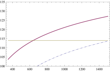
  $M_{S}$                                                           $M_{S}$

Figure 2: Left: The dependence of the one–loop lightest Higgs boson mass on $M_{S}$ for $\tan\beta=2$. Right: The one–loop mass of the lightest CP–even Higgs state versus $M_{S}$ for $\tan\beta=3$. The solid and dashed–dotted lines correspond to $X_{t}=2\,M_{S}$ and $X_{t}=M_{S}$ respectively. The horizontal line represents the current LEP limit.

Recent studies indicate that in the MSSM the scenarios with the light Higgs pseudoscalar ($m_{A}\sim 100\,\mbox{GeV}$) are almost ruled out by LEP. Since $m_{A}$ tend to be large the SM–like Higgs boson must be relatively heavy. At the same time, as it has been already mentioned, the tree–level mass of the lightest Higgs boson in the MSSM does not exceed $M_{Z}\simeq 91\,\mbox{GeV}$. As a consequence in order to satisfy LEP constraints large contribution of loop corrections to the mass of the lightest CP–even Higgs state is required. When SUSY breaking scale $M_{S}$ is considerably larger than $M_{Z}$ and $m_{Q}^{2}\simeq m_{U}^{2}\simeq M_{S}^{2}$ the contribution of the one–loop corrections to $m_{h_{1}}^{2}$ in the leading approximation can be written as

$$\Delta^{(1)}_{11}\simeq\frac{3M_{t}^{4}}{2\pi^{2}v^{2}}\left[\frac{X_{t}^{2}}{M_{S}^{2}}\biggl{(}1-\frac{1}{12}\frac{X_{t}^{2}}{M_{S}^{2}}\biggr{)}+\ln\biggl{(}\frac{M_{S}^{2}}{m_{t}^{2}}\biggr{)}\right]\,.$$ (113)

The large values of $\Delta^{(1)}_{11}\sim M_{Z}^{2}$ can be obtained only if $M_{S}\gg m_{t}$ and the ratio $|X_{t}/M_{S}|$ is also large. The contribution of the one–loop corrections (113) attains its maximal value for $X_{t}^{2}=6\,M_{S}^{2}$. This is the so–called maximal mixing scenario. In Figs. 2a and 2b the dependence of the one–loop lightest Higgs boson mass on the SUSY breaking scale $M_{S}$ for $\tan\beta=2$ and $\tan\beta=3$ is examined. Two different cases $X_{t}=M_{S}$ and $X_{t}=2\,M_{S}$ are considered. From Figs. 2a and 2b one can see that in order to satisfy LEP constraints $M_{S}$ should be larger than $400-600\,\mbox{GeV}$. Leading two–loop corrections reduce the SM–like Higgs mass even further. As a result larger values of the SUSY breaking scale are required to overcome LEP limit.

Large values of the soft scalar masses of the superpartners of the top quark ($m_{Q}^{2},\,m_{U}^{2}\gg M_{Z}^{2}$) tend to induce large and negative value of $m_{H_{2}}^{2}$ in the Higgs potential due to the RG flow. This leads to the fine tuning because $m_{1}^{2}$ and $m_{2}^{2}$ determine the EW scale (see Eqs. (102)). Generically the fine tuning which is required to overcome LEP constraints in the MSSM is of the order of 1% (little hierarchy problem). This fine tuning should be compared with the fine tuning in other theories which are used in particle physics. In particular, it is well known that QCD is a highly fine–tuned theory. Indeed, QCD Lagrangian should contain “$\theta$-term”

$${\cal L}_{\theta}=\theta_{\rm eff}\frac{\alpha_{s}}{8\pi}F^{\mu\nu\,a}\tilde{F}_{\mu\nu}^{a},\qquad\qquad\theta_{\rm eff}=\theta+{\rm arg\;det}\;M_{q}\,,$$ (114)

where $F^{\mu\nu\,a}$ is the gluon field strength and $\tilde{F}_{\mu\nu}^{a}\equiv\frac{1}{2}\epsilon_{\mu\nu\rho\sigma}F^{\rho\sigma\,a}$ is its dual. This term is not forbidden by the gauge invariance. On the other hand the parameter $\theta$ must be extremely small, i.e. $|\theta_{\rm eff}|\lesssim 10^{-9}$ (strong CP problem). Otherwise it results in too large value of the neutron electric dipole moment. Eqs. (114) demonstrate that so small value of $\theta_{\rm eff}$ implies enormous fine tuning which is much higher than in the MSSM.

The little hierarchy problem can be solved within SUSY models that allow to get relatively large mass of the SM–like Higgs boson ($m_{h_{1}}\gtrsim 100-110\,\mbox{GeV}$) at the tree-level. Alternatively, one can try to avoid stringent LEP constraints by allowing exotic decays of the lightest Higgs particle. If usual branching ratios of the lightest Higgs state are dramatically reduced then the lower LEP bound on the SM–like Higgs mass may become inapplicable. In this case the lightest Higgs boson can be still relatively light so that large contribution of loop corrections is not required. Both possibilities mentioned above imply the presence of new particles and interactions. These new particles and interactions can be also used to solve the so-called $\mu$ problem. This problem arises when MSSM gets incorporated into supergravity and/or GUT models. Within these models the parameter $\mu$ is expected to be either zero or of the order of Planck/GUT scale. At the same time in order to provide the correct pattern of the EWSB $\mu$ is required to be of the order of the EW scale.

5.2 Higgs sector of the NMSSM

In the simplest extension of the MSSM, the Next–to–Minimal Supersymmetric Standard Model (NMSSM), the superpotential is invariant with respect to the discrete transformations $\Phi_{i}\to e^{2\pi i/3}\Phi_{i}$ of the $Z_{3}$ group (for recent review see [53]). The term $\mu(H_{1}H_{2})$ does not meet this requirement. Therefore it is replaced in the superpotential by

$$W_{H}=\lambda S(H_{1}H_{2})+\frac{1}{3}\kappa S^{3}\,,$$ (115)

where $S$ is an additional superfield which is a singlet with respect to $SU(2)_{W}$ and $U(1)_{Y}$ gauge transformations. A spontaneous breakdown of the EW symmetry leads to the emergence of the VEV of extra singlet field $<S>=s/\sqrt{2}$ and an effective $\mu$ parameter is generated ($\mu=\lambda s/\sqrt{2}$).

The potential energy of the Higgs field interaction can be written as a sum

$$V=V_{F}+V_{D}+V_{soft}+\Delta V\,,$$ (116)

$$V_{F}=\lambda^{2}|S|^{2}(|H_{1}|^{2}+|H_{2}|^{2})+\lambda^{2}|(H_{1}H_{2})|^{2}\qquad\qquad$$

$$\qquad\qquad+\lambda\kappa\left[S^{*2}(H_{1}H_{2})+h.c.\right]+\kappa^{2}|S|^{4}\,,$$ (117)

$$V_{D}=\frac{g_{2}^{2}}{8}\left(H_{1}^{+}\sigma_{a}H_{1}+H_{2}^{+}\sigma_{a}H_{2}\right)^{2}+\frac{{g^{\prime}}^{2}}{8}\left(|H_{1}|^{2}-|H_{2}|^{2}\right)^{2}\,,$$ (118)

$$V_{soft}=m_{1}^{2}|H_{1}|^{2}+m_{2}^{2}|H_{2}|^{2}+m_{S}^{2}|S|^{2}\qquad\qquad$$

$$\qquad\qquad+\left[\lambda A_{\lambda}S(H_{1}H_{2})+\frac{\kappa}{3}A_{\kappa}S^{3}+h.c.\right]\,.$$ (119)

At the tree level the Higgs potential (116) is described by the sum of the first three terms. $V_{F}$ and $V_{D}$ are the $F$ and $D$ terms. Their structure is fixed by the superpotential (115) and the EW gauge interactions in the common manner. The soft SUSY breaking terms are collected in $V_{soft}$. The set of soft SUSY breaking parameters involves soft masses $m_{1}^{2},\,m_{2}^{2},\,m_{S}^{2}$ and trilinear couplings $A_{\kappa},\,A_{\lambda}$. The last term in Eq. (116), $\Delta V$, corresponds to the contribution of loop corrections. In the leading one–loop approximation $\Delta V$ in the NMSSM is given by Eqs. (103)–(104) in which $\mu$ has to be replaced by $\lambda s/\sqrt{2}$. Further we assume that $\lambda$, $\kappa$ and all soft SUSY breaking parameters are real so that CP is conserved.

At the physical vacuum of the Higgs potential

$$<H_{1}>=\frac{1}{\sqrt{2}}\left(\begin{array}[]{c}v_{1}\\ 0\end{array}\right),\quad<H_{2}>=\frac{1}{\sqrt{2}}\left(\begin{array}[]{c}0\\ v_{2}\end{array}\right)\,,\quad<S>=\frac{s}{\sqrt{2}}\,.$$ (120)

The equations for the extrema of the full Higgs boson effective potential in the directions (120) in the field space are given by

$$\frac{\partial V}{\partial s}=\left(m_{S}^{2}+\frac{\lambda^{2}}{2}(v_{1}^{2}+v_{2}^{2})-\lambda\kappa v_{1}v_{2}\right)s-\frac{\lambda A_{\lambda}}{\sqrt{2}}v_{1}v_{2}\qquad\qquad$$

$$\qquad\qquad+\frac{\kappa A_{\kappa}}{\sqrt{2}}s^{2}+\kappa^{2}s^{3}+\frac{\partial\Delta V}{\partial s}=0\,,$$ (121)

$$\frac{\partial V}{\partial v_{1}}=\left(m_{1}^{2}+\frac{\lambda^{2}}{2}(v_{2}^{2}+s^{2})+\frac{\bar{g}^{2}}{8}(v_{1}^{2}-v_{2}^{2})\right)v_{1}\qquad\qquad\qquad$$

$$\qquad\qquad-\left(\frac{\lambda\kappa}{2}s^{2}+\frac{\lambda A_{\lambda}}{\sqrt{2}}s\right)v_{2}+\frac{\partial\Delta V}{\partial v_{1}}=0\,,$$ (122)

$$\frac{\partial V}{\partial v_{2}}=\left(m_{2}^{2}+\frac{\lambda^{2}}{2}(v_{1}^{2}+s^{2})+\frac{\bar{g}^{2}}{8}(v_{2}^{2}-v_{1}^{2})\right)v_{2}\qquad\qquad\qquad$$

$$\qquad\qquad-\left(\frac{\lambda\kappa}{2}s^{2}+\frac{\lambda A_{\lambda}}{\sqrt{2}}s\right)v_{1}+\frac{\partial\Delta V}{\partial v_{2}}=0\,.$$ (123)

As in the MSSM upon the breakdown of the EW symmetry three goldstone modes ($G^{\pm}$ and $G^{0}$) emerge, and are absorbed by the $W^{\pm}$ and $Z$ bosons. In the field space basis rotated by an angle $\beta$ with respect to the initial direction, i.e.

$$\mbox{Im}\,H_{1}^{0}=(P\sin\beta+G^{0}\cos\beta)/\sqrt{2}\,,\qquad H_{2}^{+}=H^{+}\cos\beta-G^{+}\sin\beta\,,$$

$$\mbox{Im}\,H_{2}^{0}=(P\cos\beta-G^{0}\sin\beta)/\sqrt{2}\,,\qquad H_{1}^{-}=G^{-}\cos\beta+H^{-}\sin\beta\,,$$

$$\mbox{Re}\,H_{1}^{0}=(h\cos\beta-H\sin\beta+v_{1})/\sqrt{2}\,,\, \mbox{Im}\,S=P_{S}/\sqrt{2}\,,\qquad\qquad\qquad$$

$$\mbox{Re}\,H_{2}^{0}=(h\sin\beta+H\cos\beta+v_{2})/\sqrt{2}\,,\, \mbox{Re}\,S=(s+N)/\sqrt{2}\,,\qquad\qquad$$ (124)

these unphysical degrees of freedom decouple and the mass terms in the Higgs boson potential can be written as follows

$$V_{mass}=M_{H^{\pm}}^{2}H^{+}H^{-}+\frac{1}{2}(P\,\,P_{S})\,\tilde{M}^{2}\left(\begin{array}[]{c}P\\ P_{S}\end{array}\right)+\frac{1}{2}(H\,\,h\,\,N)\,M^{2}\left(\begin{array}[]{c}H\\ h\\ N\end{array}\right)\,.$$ (125)

From the conditions for the extrema (121)–(123) one can express $m_{S}^{2}$, $m_{1}^{2}$, $m_{2}^{2}$ via other fundamental parameters, $\tan\beta$ and $s$. Substituting the obtained relations for the soft masses in the $2\times 2$ CP-odd mass matrix $\tilde{M}^{2}_{ij}$ we get:

$$\tilde{M}_{11}^{2}=m_{A}^{2}=\frac{4\mu^{2}}{\sin^{2}2\beta}\left(x-\frac{\kappa}{2\lambda}\sin 2\beta\right)+\tilde{\Delta}_{11}\,,$$

$$\tilde{M}_{22}^{2}=\frac{\lambda^{2}v^{2}}{2}x+\frac{\lambda\kappa}{2}v^{2}\sin 2\beta-3\frac{\kappa}{\lambda}A_{\kappa}\mu+\tilde{\Delta}_{22}\,,$$ (126)

$$\tilde{M}_{12}^{2}=\tilde{M}_{21}^{2}=\sqrt{2}\lambda v\mu\left(\frac{x}{\sin 2\beta}-2\frac{\kappa}{\lambda}\right)+\tilde{\Delta}_{12}\,,$$

where $x=\displaystyle\frac{1}{2\mu}\left(A_{\lambda}+2\frac{\kappa}{\lambda}\mu\right)\sin 2\beta$, $\mu=\displaystyle\frac{\lambda s}{\sqrt{2}}$ and $\tilde{\Delta}_{ij}$ are contributions of the loop corrections to the mass matrix elements. The mass matrix (126) can be easily diagonalized. The corresponding eigenvalues are given by

$$m^{2}_{A_{2},A_{1}}=\frac{1}{2}\left(\tilde{M}^{2}_{11}+\tilde{M}^{2}_{22}\pm\sqrt{(\tilde{M}^{2}_{11}-\tilde{M}^{2}_{22})^{2}+4\tilde{M}^{4}_{12}}\right)~{}.$$ (127)

Because the charged components of the Higgs doublets are not mixed with the neutral Higgs states the charged Higgs fields $H^{\pm}$ are already physical mass eigenstates with

$$M_{H^{\pm}}^{2}=m_{A}^{2}-\frac{\lambda^{2}v^{2}}{2}+M_{W}^{2}+\Delta_{\pm}.$$ (128)

Here $\Delta_{\pm}$ includes loop corrections to the charged Higgs mass.

In the rotated basis $H\,,h\,,N$ the mass matrix of the CP–even Higgs sector takes the form [50],[54]:

$$M^{2}=\left(\begin{array}[]{ccc}M_{11}^{2}&M_{12}^{2}&M_{13}^{2}\\[5.69054pt] M_{21}^{2}&M_{22}^{2}&M_{23}^{2}\\[5.69054pt] M_{31}^{2}&M_{32}^{2}&M_{33}^{2}\end{array}\right)=\left(\begin{array}[]{ccc}\displaystyle\frac{1}{v^{2}}\frac{\partial^{2}V}{\partial^{2}\beta}&\displaystyle\frac{1}{v}\frac{\partial^{2}V}{\partial v\partial\beta}&\displaystyle\frac{1}{v}\frac{\partial^{2}V}{\partial s\partial\beta}\\[5.69054pt] \displaystyle\frac{1}{v}\frac{\partial^{2}V}{\partial v\partial\beta}&\displaystyle\frac{\partial^{2}V}{\partial v^{2}}&\displaystyle\frac{\partial^{2}V}{\partial v\partial s}\\[5.69054pt] \displaystyle\frac{1}{v}\frac{\partial^{2}V}{\partial s\partial\beta}&\displaystyle\frac{\partial^{2}V}{\partial v\partial s}&\displaystyle\frac{\partial^{2}V}{\partial^{2}s}\end{array}\right)~{},$$ (129)

$$\begin{array}[]{rcl}M_{11}^{2}&=&\displaystyle m_{A}^{2}+\left(\frac{\bar{g}^{2}}{4}-\frac{\lambda^{2}}{2}\right)v^{2}\sin^{2}2\beta+\Delta_{11}\,,\\ M_{22}^{2}&=&\displaystyle M_{Z}^{2}\cos^{2}2\beta+\frac{\lambda^{2}}{2}v^{2}\sin^{2}2\beta+\Delta_{22}\,,\\ M_{33}^{2}&=&\displaystyle 4\frac{\kappa^{2}}{\lambda^{2}}\mu^{2}+\frac{\kappa}{\lambda}A_{\kappa}\mu+\frac{\lambda^{2}v^{2}}{2}x-\frac{\kappa\lambda}{2}v^{2}\sin 2\beta+\Delta_{33}\,,\\ M_{12}^{2}&=&M_{21}^{2}=\displaystyle\left(\frac{\lambda^{2}}{4}-\frac{\bar{g}^{2}}{8}\right)v^{2}\sin 4\beta+\Delta_{12}\,,\\ M_{13}^{2}&=&M_{31}^{2}=-\displaystyle\frac{\sqrt{2}\lambda v\mu x\cos 2\beta}{\sin 2\beta}+\Delta_{13}\,,\\ M_{23}^{2}&=&M_{32}^{2}=\sqrt{2}\lambda v\mu(1-x)+\Delta_{23}\,,\end{array}$$ (130)

where $\Delta_{ij}$ can be calculated by differentiating $\Delta V$.

At least one Higgs state in the CP–even sector is always light. Since the minimal eigenvalue of a Hermitian matrix does not exceed its smallest diagonal element the lightest CP–even Higgs boson squared mass $m_{h_{1}}^{2}$ remains smaller than $M_{22}^{2}\sim M_{Z}^{2}$ even when the supersymmetry breaking scale is much larger than the EW scale. At the tree–level the upper bound on the lightest Higgs mass in the NMSSM was found in [56]–[57]. It differs from the theoretical bound in the MSSM only for moderate values of $\tan\beta$. In the leading two–loop approximation the lightest Higgs boson mass in the NMSSM does not exceed $135\,\mbox{GeV}$. As follows from the explicit form of the mass matrices (126) and (130) at the tree-level, the spectrum of the Higgs bosons and their couplings depend on the six parameters: $\lambda,\kappa,\mu,\tan\beta,A_{\kappa}$ and $m_{A}$ (or $x$).

First let us consider the MSSM limit of the NMSSM. Because the strength of the interaction of the extra SM singlet superfield $S$ with $H_{1}$ and $H_{2}$ is determined by the size of the coupling $\lambda$ in the superpotential (115) the MSSM expressions for the Higgs masses and couplings are reproduced when $\lambda$ tends to be zero. On the other hand the equations (122)–(123) imply that $s$ should grow with decreasing $\lambda$ as $M_{Z}/\lambda$ to ensure the correct breakdown of the EW symmetry. In the limit $\lambda\to 0$ all terms, which are proportional to $\lambda v_{i}$, in the minimization conditions (121) can be neglected and the corresponding equation takes the form:

$$s\left(m_{S}^{2}+\frac{\kappa A_{\kappa}}{\sqrt{2}}s+\kappa^{2}s^{2}\right)\simeq 0$$ (131)

The Eq. (131) has always at least one solution $s_{0}=0$. In addition two non-trivial roots arise if $A_{\kappa}^{2}>8m_{S}^{2}$. They are given by

$$s_{1,2}\simeq\frac{-A_{\kappa}\pm\sqrt{A_{\kappa}^{2}-8m_{S}^{2}}}{2\sqrt{2}\kappa}\,\,.$$ (132)

When $m_{S}^{2}>0$ the root $s_{0}=0$ corresponds to the local minimum of the Higgs potential (116)–(119) that does not lead to the acceptable solution of the $\mu$–problem. The second non-trivial vacuum, that appears if $A_{\kappa}^{2}>8m_{S}^{2}$, remains unstable for $A_{\kappa}^{2}<9m_{S}^{2}$. Larger absolute values of $A_{\kappa}$ $(A_{\kappa}^{2}>9m_{S}^{2})$ stabilizes the second minimum which is attained at $s=s_{1}(s_{2})$ for negative (positive) $A_{\kappa}$. From Eq. (132) it becomes clear that the increasing of $s$ can be achieved either by decreasing $\kappa$ or by raising $m_{S}^{2}$ and $A_{\kappa}$. Since there is no natural reason why $m_{S}^{2}$ and $A_{\kappa}$ should be very large while all other soft SUSY breaking terms are left in the TeV range, the values of $\lambda$ and $\kappa$ are obliged to go to zero simultaneously so that their ratio remains unchanged.

Since in the MSSM limit of the NMSSM mixing between singlet states and neutral components of the Higgs doublets is small the mass matrices (126) and (129)–(130) can be diagonalised using the perturbation theory [50],[54],[58]–[60]. At the tree–level the masses of two Higgs pseudoscalars are given by

$$m_{A_{2}}^{2}\simeq m_{A}^{2}=\frac{4\mu^{2}}{\sin^{2}2\beta}\left(x-\frac{\kappa}{2\lambda}\sin 2\beta\right)\,,\qquad m_{A_{1}}^{2}\simeq-3\frac{\kappa}{\lambda}A_{\kappa}\mu\,.$$ (133)

The masses of two CP–even Higgs bosons are the same as in the MSSM (see Eq. (109)) while the mass of the extra CP–even Higgs state, which is predominantly a SM singlet field, is set by $\frac{\kappa}{\lambda}\mu$

$$m_{h_{3}}^{2}\approx 4\frac{\kappa^{2}}{\lambda^{2}}\mu^{2}+\frac{\kappa}{\lambda}A_{\kappa}\mu+\frac{\lambda^{2}v^{2}}{2}x\sin^{2}2\beta-\frac{2\lambda^{2}v^{2}\mu^{2}(1-x)^{2}}{M_{Z}^{2}\cos^{2}2\beta}\,.$$ (134)

The parameter $A_{\kappa}$ occurs in the masses of extra scalar $m_{h_{3}}$ and pseudoscalar $m_{A_{1}}$ with opposite sign and is therefore responsible for their splitting. To ensure that the physical vacuum is a global minimum of the Higgs potential (116)–(119) and the masses-squared of all Higgs states are positive in this vacuum the parameter $A_{\kappa}$ must satisfy the following constraints

$$-3\left(\frac{\kappa}{\lambda}\mu\right)^{2}\lesssim A_{\kappa}\left(\frac{\kappa}{\lambda}\mu\right)\lesssim 0\,.$$ (135)

The experimental constraints on the SUSY parameters obtained in the MSSM remain valid in the NMSSM with small $\lambda$ and $\kappa$. For example, non–observation of any neutral Higgs particle and chargino at the LEP II imply that $\tan\beta\gtrsim 2.5$ and $|\mu|\gtrsim 90-100\,\mbox{GeV}$.

Decreasing $\kappa$ reduces the masses of extra scalar and pseudoscalar states so that for $\kappa\ll\lambda$ they can be the lightest particles in the Higgs boson spectrum. In the limit $\kappa\to 0$ the mass of the lightest pseudoscalar state vanishes. In the considered limit the Lagrangian of the NMSSM is invariant under transformations of $SU(2)\times[U(1)]^{2}$ global symmetry. Extra $U(1)$ global symmetry gets spontaneously broken by the VEV of the singlet field $S$, giving rise to a massless Goldstone boson, the Peccei–Quinn (PQ) axion. In the PQ–symmetric NMSSM astrophysical observations exclude any choice of the parameters unless one allows $s$ to be enormously large ($>10^{9}-10^{11}\,\mbox{GeV}$). These huge vacuum expectation values of the singlet field can be consistent with the EWSB only if $\lambda\sim 10^{-6}-10^{-9}$ [61]–[62]. Therefore here we restrict our consideration to small but non–zero values of $\kappa\lesssim\lambda^{2}$ when the PQ-symmetry is only slightly broken.

As evident from Eq. (134) at small values of $\kappa$ the mass–squared of the lightest Higgs scalar tends to be negative if $|\mu|$ is large and/or the auxiliary variable $x$ differs too much from unity. Due to the vacuum stability requirement, which implies the positivity of the mass–squared of all Higgs particles, $x$ has to be localized near unity, i.e.

$$1-\left|\frac{\sqrt{2}\kappa M_{Z}}{\lambda^{2}v}\right|<x<1+\left|\frac{\sqrt{2}\kappa M_{Z}}{\lambda^{2}v}\right|\,.$$ (136)

This leads to the hierarchical structure of the Higgs spectrum. Indeed, combining LEP limits on $\tan\beta$ and $\mu$ one gets that $m_{A}^{2}\gtrsim 9M_{Z}^{2}\,x$. Because of this the heaviest CP–odd, CP–even and charged Higgs bosons are almost degenerate with masses around $m_{A}\simeq\mu\tan\beta$ while the SM–like Higgs state has a mass of the order of $M_{Z}$.

$m_{A}(\mbox{GeV})$

Figure 3: One–loop masses of the CP–even Higgs bosons versus $m_{A}$ for $\lambda=0.6$, $\kappa=0.36$, $\tan\beta=3$, $\mu=150\,\mbox{GeV}$, $A_{\kappa}=135\,\mbox{GeV}$, $m_{Q}^{2}=m_{U}^{2}=M_{S}^{2}$, $X_{t}=\sqrt{6}M_{S}$ and $M_{S}=700\,\mbox{GeV}$. Solid, dashed and dashed–dotted lines correspond to the masses of the CP–even, CP–odd and charged Higgs bosons respectively.

The main features of the NMSSM Higgs spectrum discussed above are retained when the couplings $\lambda$ and $\kappa$ increase. For the appreciable values of $\kappa$ and $\lambda$ the slight breaking of the PQ–symmetry can be caused by the RG flow of these couplings from the GUT scale $M_{X}$ to $M_{Z}$. In the infrared region the solutions of the NMSSM RG equations are focused near the intersection of the Hill-type effective surface and invariant line [63]–[65]. As a result at the EW scale $\kappa/\lambda$ tend to be less than unity even when $\kappa(M_{X})>\lambda(M_{X})$ initially. In Fig. 3 the dependence of the masses of the Higgs bosons on $m_{A}$ is examined. As a representative example we fix the Yukawa couplings so that $\lambda(M_{X})=\kappa(M_{X})=2h_{t}(M_{X})=1.6$, that corresponds to $\tan\beta\gtrsim 3$, $\lambda(M_{t})=0.6$ and $\kappa(M_{t})=0.36$. In order to obtain a realistic spectrum, we include the leading one–loop corrections from the top and stop loops. From Fig. 3 it becomes clear that the requirement of stability of the physical vacuum limits the range of variations of $m_{A}$ from below and above maintaining the mass hierarchy in the Higgs spectrum. Relying on this mass hierarchy the approximate solutions for the Higgs masses and couplings can be obtained [59],[60]. The numerical results in Fig. 3 reveal that the masses of the heaviest CP–even, CP–odd and charged Higgs states are approximately degenerate while the other three neutral states are considerably lighter. The hierarchical structure of the Higgs spectrum ensures that the heaviest CP–even and CP–odd Higgs bosons are predominantly composed of $H$ and $P$. As before the lightest Higgs scalar and pseudoscalar are singlet dominated, making their observation quite problematic. The second lightest CP–even Higgs boson has a mass around $130\,\mbox{GeV}$, mimicking the lightest Higgs scalar in the MSSM. Observing two light scalars and one pseudoscalar Higgs particles but no charged Higgs boson at future colliders would yield an opportunity to differentiate the NMSSM with a slightly broken PQ–symmetry from the MSSM even if the heavy Higgs states are inaccessible.

The presence of light singlet scalar and pseudoscalar permits to weaken the LEP lower bound on the lightest Higgs boson mass. These states have reduced couplings to Z–boson that could allow them to escape the detection at LEP. On the other hand singlet scalar can mix with the SM-like superposition $h$ of the neutral components of Higgs doublets resulting in the reduction of the couplings of the second lightest Higgs scalar to $Z$–boson. This relaxes LEP constraints so that the SM-like Higgs state does not need to be considerably heavier than $100\,\mbox{GeV}$. Therefore large contribution of loop corrections to the mass of the SM-like Higgs boson is not required. Another possibility to overcome the little hierarchy problem is to allow the SM–like Higgs state to decay predominantly into two light singlet pseudoscalars $A_{1}$ (for recent review see [66]). This can be achieved because the coupling of the SM–like Higgs boson to the $b$–quark is rather small. If this coupling is substantially smaller than the coupling of the SM–like Higgs state to $A_{1}$ then the decay mode $h\to A_{1}+A_{1}$ dominates. The singlet pseudoscalar can sequentially decay into either $b\bar{b}$ or $\tau\bar{\tau}$ leading to four fermion decays of the SM–like Higgs boson. In this case, again, the corresponding Higgs eigenstate might be relatively light that permits to avoid little hierarchy problem.

$m_{h_{1}}$                                                           $m_{h_{1}}$
  
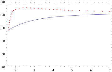
  $\tan\beta$                                                           $\tan\beta$

Figure 4: Left: Tree–level upper bound on the lightest Higgs boson mass in the MSSM and NMSSM as a function of $\tan\beta$. Right: The dependence of the two–loop upper bound on the lightest Higgs boson mass on $\tan\beta$ for $m_{t}(M_{t})=165\,\mbox{GeV}$, $m_{Q}^{2}=m_{U}^{2}=M_{S}^{2}$, $X_{t}=\sqrt{6}M_{S}$ and $M_{S}=700\,\mbox{GeV}$. The solid and dotted lines represent the theoretical restrictions on $m_{h_{1}}$ in the MSSM and NMSSM respectively.

However even when the couplings of the lightest CP–even Higgs state are almost the same as in the SM it is substantially easier to overcome LEP constraint on the mass of the SM–like Higgs boson in the NMSSM than in the MSSM. Indeed, in the NMSSM the theoretical upper bound on $m_{h_{1}}^{2}$, which is given by $M_{22}^{2}$ in Eq. (130), contains an extra term $\frac{\lambda^{2}}{2}v^{2}\sin^{2}2\beta$ which is not present in the MSSM. Due to this term the maximum possible value of the mass of the lightest Higgs scalar in the NMSSM can be considerably larger as compared with the MSSM at moderate values of $\tan\beta$. In our analysis we require the validity of perturbation theory up to the scale $M_{X}$. This sets stringent upper limit on $\lambda(M_{t})$ at low energies for each particular choice of $\tan\beta$. Using theoretical restrictions on $\lambda(M_{t})$ one can compute the the maximum possible value of $m_{h_{1}}^{2}$ for each given value of $\tan\beta$. Fig. 4 shows the dependence of the upper bound on the lightest Higgs boson mass as a function of $\tan\beta$ in the MSSM and NMSSM. From Fig. 4 one can see that at the tree–level the lightest CP–even Higgs state in the NMSSM can be considerably heavier than in the MSSM at moderate values of $\tan\beta$. As a consequence in the leading two–loop approximation it is substantially easier to get $m_{h_{1}}\gtrsim 114.4\,\mbox{GeV}$ in the NMSSM than in the MSSM for $\tan\beta=2-4$.

5.3 Higgs spectrum in the $E_{6}$ inspired SUSY models with extra $U(1)^{\prime}$ factor

Another solution to the $\mu$ problem arises within superstring inspired models based on the $E_{6}$ gauge group. At high energies $E_{6}$ can be broken $SU(3)_{C}\times SU(2)_{W}\times U(1)_{Y}\times U(1)^{\prime}$. An extra $U(1)^{\prime}$ that appears at low energies is a linear superposition of $U(1)_{\chi}$ and $U(1)_{\psi}$:

$$U(1)^{\prime}=U(1)_{\chi}\cos\theta+U(1)_{\psi}\sin\theta\,,$$ (137)

where two anomaly–free $U(1)_{\psi}$ and $U(1)_{\chi}$ symmetries are defined by: $E_{6}\to SO(10)\times U(1)_{\psi}$ , $SO(10)\to SU(5)\times U(1)_{\chi}$. If $\theta\neq 0$ or $\pi$ the extra $U(1)^{\prime}$ gauge symmetry forbids an elementary $\mu$ term but allows interaction $\lambda S(H_{1}H_{2})$ in the superpotential. After EWSB the scalar component of the SM singlet superfield $S$ acquires a non–zero VEV breaking $U(1)^{\prime}$ and an effective $\mu$ term of the required size is automatically generated.

The Higgs sector of the considered models includes two Higgs doublets as well as a SM–like singlet field $S$ that carries $U(1)^{\prime}$ charge. The Higgs effective potential can be written as

$$\begin{array}[]{rcl}V&=&V_{F}+V_{D}+V_{soft}+\Delta V\,,\\[2.84526pt] V_{F}&=&\lambda^{2}|S|^{2}(|H_{d}|^{2}+|H_{u}|^{2})+\lambda^{2}|(H_{d}H_{u})|^{2}\,,\\[2.84526pt] V_{D}&=&\displaystyle\frac{g_{2}^{2}}{8}\left(H_{d}^{\dagger}\sigma_{a}H_{d}+H_{u}^{\dagger}\sigma_{a}H_{u}\right)^{2}+\displaystyle\frac{{g^{\prime}}^{2}}{8}\left(|H_{d}|^{2}-|H_{u}|^{2}\right)^{2}\\[5.69054pt] &&+\displaystyle\frac{g^{{}^{\prime}2}_{1}}{2}\left(\tilde{Q}_{1}|H_{d}|^{2}+\tilde{Q}_{2}|H_{u}|^{2}+\tilde{Q}_{S}|S|^{2}\right)^{2}\,,\\[2.84526pt] V_{soft}&=&m_{S}^{2}|S|^{2}+m_{1}^{2}|H_{d}|^{2}+m_{2}^{2}|H_{u}|^{2}+\biggl{[}\lambda A_{\lambda}S(H_{u}H_{d})+h.c.\biggr{]}\,,\end{array}$$ (138)

where $g^{\prime}_{1}$ is $U(1)^{\prime}$ gauge coupling and $\tilde{Q}_{1}$, $\tilde{Q}_{2}$ and $\tilde{Q}_{S}$ are effective $U(1)^{\prime}$ charges of $H_{1}$, $H_{2}$ and $S$ respectively. In Eq. (138) $V_{F}$ and $V_{D}$ are the $F$ and $D$ terms, $V_{soft}$ contains a set of soft SUSY breaking terms while $\Delta V$ represents the contribution of loop corrections.

At the physical vacuum the Higgs fields acquire VEVs given by Eq. (120) thus breaking the $SU(2)_{W}\times U(1)_{Y}\times U(1)^{\prime}$ symmetry to $U(1)_{em}$. As a result two CP–odd and two charged Goldstone modes in the Higgs sector are absorbed by the $Z$, $Z^{\prime}$ and $W^{\pm}$ gauge bosons so that only six physical degrees of freedom are left. They form one CP–odd, three CP–even and two charged states. The masses of the CP–odd and charged Higgs bosons can be written as

$$m_{A}^{2}=\frac{2\lambda^{2}s^{2}x}{\sin^{2}2\beta}+O(M_{Z}^{2})\,,\qquad\qquad m^{2}_{H^{\pm}}=m_{A}^{2}+O(M_{Z}^{2})\,,$$ (139)

where $x=\frac{A_{\lambda}}{\sqrt{2}\lambda s}\sin 2\beta$ . The masses of two heaviest CP–even states are set by $M_{Z^{\prime}}$ and $m_{A}$, i.e.

$$m^{2}_{h_{3}}=m_{A}^{2}+O(M_{Z}^{2})\,,\qquad\qquad m^{2}_{h_{2}}=M_{Z^{\prime}}^{2}+O(M_{Z}^{2})\,,$$ (140)

where $M_{Z^{\prime}}\simeq g^{{}^{\prime}}_{1}\tilde{Q}_{S}s$. The lightest CP–even Higgs boson has a mass which is less than

$$m^{2}_{h_{1}}\lesssim\frac{\lambda^{2}}{2}v^{2}\sin^{2}2\beta+M_{Z}^{2}\cos^{2}2\beta+g^{{}^{\prime}2}_{1}v^{2}\biggl{(}\tilde{Q}_{1}\cos^{2}\beta+\tilde{Q}_{2}\sin^{2}\beta\biggr{)}^{2}+\Delta\,.$$ (141)

In Eq. (141) $\Delta$ represents the contribution of loop corrections. Since the mass of the $Z^{\prime}$ boson in the $E_{6}$ inspired models has to be heavier than $800-900\,\mbox{GeV}$ at least one CP–even Higgs state, which is singlet dominated, is always heavy. If $m_{A}<M_{Z^{\prime}}$ then we get MSSM–type Higgs spectrum. When $m_{A}>M_{Z^{\prime}}$ the heaviest CP–even, CP–odd and charged states are almost degenerate with masses around $m_{A}$. In this case the lightest Higgs state is predominantly the SM-like superposition $h$ of the neutral components of Higgs doublets.

Recently the detailed analysis of the Higgs sector was performed within a particular $E_{6}$ inspired SUSY model with an extra $U(1)_{N}$ gauge symmetry that corresponds to $\theta=\arctan\sqrt{15}$ [67]-[68]. The extra $U(1)_{N}$ gauge symmetry is defined such that right–handed neutrinos do not participate in the gauge interactions. Only in this Exceptional Supersymmetric Standard Model (E₆SSM) right–handed may be superheavy, shedding light on the origin of the mass hierarchy in the lepton sector and providing a mechanism for the generation of the baryon asymmetry in the Universe via leptogenesis [69]. To ensure anomaly cancellation the particle content of the E₆SSM is extended to include three complete fundamental $27$ representations of $E_{6}$. In addition to the complete $27_{i}$ multiplets the low energy particle spectrum of the E₆SSM is supplemented by $SU(2)_{W}$ doublet $H^{\prime}$ and anti-doublet $\overline{H}^{\prime}$ states from extra $27^{\prime}$ and $\overline{27^{\prime}}$ to preserve gauge coupling unification. The unification of gauge couplings in the considered model can be achieved for any phenomenologically acceptable value of $\alpha_{3}(M_{Z})$ consistent with the measured low energy central value [70]. The Higgs spectrum within the E₆SSM was studied in [67]-[68], [71]–[72]. It was argued that even at the tree level the lightest Higgs boson mass in this model can be larger than $120\,\mbox{GeV}$. Therefore nonobservation of the Higgs boson at LEP does not cause any trouble for the E₆SSM, even at tree–level. In the leading two–loop approximation the mass of the lightest CP–even Higgs boson in the considered model does not exceed $150-155\,\mbox{GeV}$ [67]. The presence of light exotic particles in the E₆SSM spectrum lead to the nonstandard decays of the SM–like Higgs boson which were discussed in [73].

References

- [1] S. R. Coleman, J. Mandula, All possible symmetries of the S matrix Phys. Rev. 159 (1967) 1251.
- [2] P. Nath, R. L. Arnowitt, “Generalized Supergauge Symmetry As A New Framework For Unified Gauge Theories,” Phys. Lett. B 56 (1975) 177.
- [3] D. Z. Freedman, P. van Nieuwenhuizen, S. Ferrara, “Progress Toward A Theory Of Supergravity,” Phys. Rev. D 13 (1976) 3214.
- [4] S. Deser, B. Zumino,“Consistent Supergravity,” Phys. Lett. B 62 (1976) 335.
- [5] D. Bailin, A. Love, ”Supersymmetric gauge field theory and string theory”, Institute of Physics Publishing, 1994.
- [6] J. Wess, J. Bagger, “Supersymmetry and supergravity,” Princeton, USA: Univ. Pr., 1992.
- [7] P. C. West, “Introduction to Supersymmetry and Supergravity,” Singapore, Singapore: World Scientific, 1986.
- [8] S. Weinberg, “The quantum theory of fields. Vol. 3: Supersymmetry,” Cambridge, UK: Univ. Pr., 2000.
- [9] H. Baer, X. Tata, “Weak scale supersymmetry: From superfields to scattering events,” Cambridge, UK: Univ. Pr., 2006.
- [10] S. J. Gates, M. T. Grisaru, M. Rocek, W. Siegel, “Superspace, or one thousand and one lessons in supersymmetry,” Front. Phys. 58 (1983) 1 [arXiv:hep-th/0108200].
- [11] S. P. Martin, “A Supersymmetry Primer,” arXiv:hep-ph/9709356.
- [12] D. I. Kazakov, “Beyond the standard model (in search of supersymmetry),” arXiv:hep-ph/0012288; “Beyond the standard model,” arXiv:hep-ph/0411064.
- [13] A. V. Gladyshev, D. I. Kazakov, “Supersymmetry and LHC,” Phys. Atom. Nucl. 70 (2007) 1553 [arXiv:hep-ph/0606288].
- [14] A. Signer, “Abc of SUSY,” J. Phys. G 36 (2009) 073002 [arXiv:0905.4630 [hep-ph]].
- [15] M. E. Peskin, “Supersymmetry in Elementary Particle Physics,” arXiv:0801.1928 [hep-ph].
- [16] M. A. Shifman, A. I. Vainshtein, “Instantons versus supersymmetry: Fifteen years later,” arXiv:hep-th/9902018.
- [17] N. Polonsky, “Supersymmetry: Structure And Phenomena. Extensions Of The Standard Model,” Lect. Notes Phys. M68 (2001) 1 [arXiv:hep-ph/0108236].
- [18] M. A. Luty, “2004 TASI lectures on supersymmetry breaking,” arXiv:hep-th/0509029.
- [19] G. L. Kane, “Weak scale supersymmetry: A top-motivated-bottom-up approach,” arXiv:hep-ph/0202185.
- [20] K. A. Olive, “Introduction to supersymmetry: Astrophysical and phenomenological constraints,” arXiv:hep-ph/9911307.
- [21] I. J. R. Aitchison, “Supersymmetry and the MSSM: An Elementary introduction,” arXiv:hep-ph/0505105.
- [22] M. Drees, “An Introduction to supersymmetry,” arXiv:hep-ph/9611409.
- [23] J. D. Lykken, “Introduction to supersymmetry,” arXiv:hep-th/9612114.
- [24] M. Dine, “Supersymmetry Breaking at Low Energies,” Nucl. Phys. Proc. Suppl. 192-193 (2009) 40 [arXiv:0901.1713 [hep-ph]].
- [25] K. A. Intriligator, N. Seiberg, “Lectures on Supersymmetry Breaking,” Class. Quant. Grav. 24 (2007) S741 [arXiv:hep-ph/0702069].
- [26] H. P. Nilles, “Supersymmetry, Supergravity And Particle Physics,” Phys. Rept. 110 (1984) 1.
- [27] H. E. Haber, G. L. Kane, “The Search For Supersymmetry: Probing Physics Beyond The Standard Model,” Phys. Rept. 117 (1985) 75.
- [28] A. B. Lahanas, D. V. Nanopoulos, “The Road to No Scale Supergravity,” Phys. Rept. 145 (1987) 1.
- [29] D. J. H. Chung, L. L. Everett, G. L. Kane, S. F. King, J. D. Lykken, L. T. Wang, “The soft supersymmetry-breaking Lagrangian: Theory and applications,” Phys. Rept. 407 (2005) 1 [arXiv:hep-ph/0312378].
- [30] J. Wess and B. Zumino, “Supergauge Invariant Extension Of Quantum Electrodynamics,” Nucl. Phys. B 78 (1974) 1.
- [31] E. Witten, “Dynamical Breaking Of Supersymmetry,” Nucl. Phys. B 188 (1981) 513.
- [32] N. Sakai, “Naturalness In Supersymmetric ’Guts’,” Z. Phys. C 11 (1981) 153.
- [33] S. Dimopoulos, H. Georgi, “Softly Broken Supersymmetry And SU(5),” Nucl. Phys. B 193 (1981) 150.
- [34] R. K. Kaul, P. Majumdar, “Cancellation Of Quadratically Divergent Mass Corrections In Globally Supersymmetric Spontaneously Broken Gauge Theories,” Nucl. Phys. B 199 (1982) 36.
- [35] L. Girardello, M. T. Grisaru, “Soft Breaking Of Supersymmetry,” Nucl. Phys. B 194 (1982) 65.
- [36] J. R. Ellis, S. Kelley, D. V. Nanopoulos, “Probing the desert using gauge coupling unification,” Phys. Lett. B 260 (1991) 131.
- [37] P. Langacker, M. Luo, “Implications of precision electroweak experiments for , , and grand unification,” Phys. Rev. D 44 (1991) 817.
- [38] U. Amaldi, W. de Boer, H. Furstenau, “Comparison of grand unified theories with electroweak and strong coupling constants measured at LEP,” Phys. Lett. B 260 (1991) 447.
- [39] F. Anselmo, L. Cifarelli, A. Peterman, A. Zichichi, “The Effective experimental constraints on M (susy) and M (gut),” Nuovo Cim. A 104 (1991) 1817.
- [40] H. Georgi, S. L. Glashow, “Unity Of All Elementary Particle Forces,” Phys. Rev. Lett. 32 (1974) 438.
- [41] M. B. Green, J. H. Schwarz, E. Witten, “Superstring Theory,” Cambridge, UK: Univ. Pr., 1987.
- [42] P. Langacker, N. Polonsky, “The Strong coupling, unification, and recent data,” Phys. Rev. D 52 (1995) 3081 [arXiv:hep-ph/9503214].
- [43] P. H. Chankowski, Z. Pluciennik, S. Pokorski, C. E. Vayonakis, “Gauge coupling unification in GUT and string models,” Phys. Lett. B 358 (1995) 264 [arXiv:hep-ph/9506393].
- [44] J. Bagger, K. T. Matchev, D. Pierce, “Precision corrections to supersymmetric unification,” Phys. Lett. B 348 (1995) 443 [arXiv:hep-ph/9501277].
- [45] W. de Boer, C. Sander, “Global electroweak fits and gauge coupling unification,” Phys. Lett. B 585 (2004) 276 [arXiv:hep-ph/0307049].
- [46] L. E. Ibanez, G. G. Ross, “SU(2)-L X U(1) Symmetry Breaking As A Radiative Effect Of Supersymmetry Breaking In Guts,” Phys. Lett. B 110 (1982) 215.
- [47] J. R. Ellis, D. V. Nanopoulos, K. Tamvakis, “Grand Unification In Simple Supergravity,” Phys. Lett. B 121 (1983) 123.
- [48] J. R. Ellis, J. S. Hagelin, D. V. Nanopoulos, K. Tamvakis, “Weak Symmetry Breaking By Radiative Corrections In Broken Supergravity,” Phys. Lett. B 125 (1983) 275.
- [49] L. Alvarez-Gaume, J. Polchinski, M. B. Wise, “Minimal Low-Energy Supergravity,” Nucl. Phys. B 221 (1983) 495.
- [50] P. A. Kovalenko, R. B. Nevzorov, K. A. Ter-Martirosian, “Masses of Higgs bosons in supersymmetric theories,” Phys. Atom. Nucl. 61 (1998) 812.
- [51] K. Inoue, A. Kakuto, H. Komatsu, S. Takeshita, “Low-Energy Parameters And Particle Masses In A Supersymmetric Grand Unified Model,” Prog. Theor. Phys. 67 (1982) 1889.
- [52] R. A. Flores, M. Sher, “Higgs Masses In The Standard, Multi-Higgs And Supersymmetric Models,” Annals Phys. 148 (1983) 95.
- [53] U. Ellwanger, C. Hugonie, A. M. Teixeira, “The Next-to-Minimal Supersymmetric Standard Model,” Phys. Rept. 496 (2010) 1 [arXiv:0910.1785 [hep-ph]].
- [54] R. B. Nevzorov, K. A. Ter-Martirosyan, M. A. Trusov, “Higgs bosons in the simplest SUSY models,” Phys. Atom. Nucl. 65 (2002) 285 [arXiv:hep-ph/0105178].
- [55] S. Hesselbach, D. J. Miller, G. Moortgat-Pick, R. Nevzorov, M. Trusov, “Theoretical upper bound on the mass of the LSP in the MNSSM,” Phys. Lett. B 662 (2008) 199 [arXiv:0712.2001 [hep-ph]].
- [56] L. Durand, J. L. Lopez, “Upper Bounds on Higgs and Top Quark Masses in the Flipped SU(5) x U(1) Superstring Model,” Phys. Lett. B 217 (1989) 463.
- [57] M. Drees, “Supersymmetric Models with Extended Higgs Sector,” Int. J. Mod. Phys. A 4 (1989) 3635.
- [58] R. B. Nevzorov, M. A. Trusov, “Particle spectrum in the modified NMSSM in the strong Yukawa coupling limit,” J. Exp. Theor. Phys. 91 (2000) 1079 [arXiv:hep-ph/0106351].
- [59] D. J. Miller, R. Nevzorov, P. M. Zerwas, “The Higgs sector of the next-to-minimal supersymmetric standard model,” Nucl. Phys. B 681 (2004) 3 [arXiv:hep-ph/0304049].
- [60] R. Nevzorov, D. J. Miller, “Approximate solutions for the Higgs masses and couplings in the NMSSM,” [arXiv:hep-ph/0411275].
- [61] D. J. Miller, R. Nevzorov, “The Peccei-Quinn axion in the next-to-minimal supersymmetric standard model,” [arXiv:hep-ph/0309143].
- [62] D. J. Miller, S. Moretti, R. Nevzorov, “Higgs bosons in the NMSSM with exact and slightly broken PQ-symmetry,” [arXiv:hep-ph/0501139].
- [63] R. B. Nevzorov, M. A. Trusov, “Infrared quasi-fixed solutions in the NMSSM,” Phys. Atom. Nucl. 64 (2001) 1299 [arXiv:hep-ph/0110363].
- [64] R. B. Nevzorov, M. A. Trusov, “Renormalization of the soft SUSY breaking terms in the strong Yukawa coupling limit in the NMSSM,” Phys. Atom. Nucl. 64 (2001) 1513 [arXiv:hep-ph/0112301].
- [65] R. B. Nevzorov, M. A. Trusov, “Quasi-fixed point scenario in the modified NMSSM,” Phys. Atom. Nucl. 65 (2002) 335 [arXiv:hep-ph/0301179].
- [66] S. Chang, R. Dermisek, J. F. Gunion, N. Weiner, “Nonstandard Higgs Boson Decays,” Ann. Rev. Nucl. Part. Sci. 58 (2008) 75 [arXiv:0801.4554 [hep-ph]].
- [67] S. F. King, S. Moretti, R. Nevzorov, “Theory and phenomenology of an exceptional supersymmetric standard model,” Phys. Rev. D 73 (2006) 035009 [arXiv:hep-ph/0510419].
- [68] S. F. King, S. Moretti, R. Nevzorov, “Exceptional supersymmetric standard model,” Phys. Lett. B 634 (2006) 278 [arXiv:hep-ph/0511256].
- [69] S. F. King, R. Luo, D. J. Miller, R. Nevzorov, “Leptogenesis in the Exceptional Supersymmetric Standard Model: flavour dependent lepton asymmetries,” JHEP 0812 (2008) 042 [arXiv:0806.0330 [hep-ph]].
- [70] S. F. King, S. Moretti, R. Nevzorov, “Gauge Coupling Unification in the Exceptional Supersymmetric Standard Model,” Phys. Lett. B 650 (2007) 57 [arXiv:hep-ph/0701064].
- [71] S. F. King, S. Moretti, R. Nevzorov, “Spectrum of Higgs particles in the ESSM,” [arXiv:hep-ph/0601269].
- [72] S. F. King, S. Moretti, R. Nevzorov, “E6SSM,” AIP Conf. Proc. 881 (2007) 138 [arXiv:hep-ph/0610002].
- [73] J. P. Hall, S. F. King, R. Nevzorov, S. Pakvasa, M. Sher, “Novel Higgs Decays and Dark Matter in the E6SSM,” [arXiv:1012.5114 [hep-ph]].