SSGSS: The Spitzer SDSS GALEX Spectroscopic Survey

Abstract

The Spitzer SDSS GALEX Spectroscopic Survey (SSGSS) provides a new sample of 101 star-forming galaxies at $z<0.2$ with unprecedented multi-wavelength coverage. New mid- to far-infrared spectroscopy from the Spitzer Space Telescope is added to a rich suite of previous imaging and spectroscopy, including ROSAT, GALEX, SDSS, 2MASS, and Spitzer/SWIRE. Sample selection ensures an even coverage of the full range of normal galaxy properties, spanning two orders of magnitude in stellar mass, colour, and dust attenuation. In this paper we present the SSGSS data set, describe the science drivers, and detail the sample selection, observations, data reduction, and quality assessment. Also in this paper, we compare the shape of the thermal continuum and the degree of silicate absorption of these typical, star-forming galaxies to those of starburst galaxies. We investigate the link between star formation rate, infrared luminosity, and total PAH luminosity, with a view to calibrating the latter for SED models in photometric samples and at high redshift. Lastly, we take advantage of the 5-40 µm spectroscopic and far infrared photometric coverage of this sample to perform detailed fitting of the Draine et al. (2007) dust models, and investigate the link between dust mass and star formation history and AGN properties.

1 Introduction

Spectroscopy in the mid- to far-infrared is emerging as a critical tool for understanding the physical properties of galaxies, and is the missing link in the new era of very large multi-wavelength spectroscopic galaxy surveys. This spectral region is dominated by emission from interstellar gas and dust, largely powered by active star formation. Observation of this reprocessed starlight enables measurement of embedded star formation that is inaccessible to ultraviolet (UV) or optical diagnostics. Spectroscopy in the infrared (IR) also directly probes the makeup and physical state of the interstellar medium (ISM) through the shape of the thermal continuum, aromatic molecular bands and a wealth of emission lines.

The improved understanding of star formation on a galactic scale granted by IR spectroscopy is increasingly important as we strive to understand the evolution of cosmic star formation, and in particular its decline since z$\sim$1. While IR spectroscopy has enabled substantial progress in mapping the most intensely star-forming (SF) galaxies in the local universe, these galaxies are not the principal stellar factories of the current epoch, nor are they the closest analogs to the dominant sources of star-formation at its cosmic peak.

At z$\sim$1, luminous infrared as well as ultra-luminous infrared galaxies (LIRGS and ULIRGS) appear to dominate star-forming activity (Le Floc’h et al., 2005), in stark contrast to the local universe where lower-luminosity ’normal’ galaxies contribute the bulk of current star formation. However a number of independent studies (Melbourne, Koo & Le Floc’h, 2005; Bell et al., 2005; Noeske et al., 2007; Zheng et al., 2007) show that these z$\sim$1 LIRGS and ULIRGS do not display the signs of violent interactions observed in their local counterparts. In fact, it appears that over much of cosmic history the bulk of stars were formed in galaxies dynamically similar to normal, disk-dominated galaxies at low redshift.

Thus, low-redshift disk galaxies are important laboratories of cosmic star formation—both in their own right and as dynamical analogs of higher redshift LIRGS and ULIRGS. The Sloan Digital Sky Survey (SDSS) (York et al., 2000) has enabled dramatic strides in our understanding of this galaxy population (Bell et al., 2003; Brinchmann et al., 2004; Kauffmann et al., 2003a, 2004; Blanton et al., 2003a; Balogh et al., 2004), and GALEX observations of the SDSS sample has provided a powerful additional lever arm for understanding—and selecting for—the star formation properties of these galaxies (e.g. Heckman et al. 2005; Yi et al. 2005.

Mid-IR (MIR) to far-IR (FIR) spectroscopy is now the key missing ingredient. Its addition to the GALEX and SDSS data allows a thorough accounting of star formation, opens up a wealth of new diagnostics, and grants the potential to self-consistently treat stellar populations and dust absorption and emission in models (e.g. Da Cunha, Charlot, & Elbaz 2008). A sample of star-forming galaxies spanning a representative range of physical properties with comprehensive multiwavelength coverage from the far-UV (FUV) to the FIR is necessary.

The Spitzer-SDSS-GALEX Spectroscopy Survey (SSGSS) provides such a sample. Selecting from the low-extinction Lockman Hole within the Sloan+GALEX footprint, FUV and optical diagnostics are used to define a broad, representative sample of 100 normal, star-forming galaxies between redshifts 0 and 0.2, boasting rich, multi-wavelength coverage. Deep Spitzer low-resolution spectroscopy has been obtained for the entire sample, and high-resolution spectroscopy for the brightest 33 galaxies.

In this paper we describe the SSGSS dataset. In Section 2 we outline the scientific motivation and goals of the survey, in Section 3 we describe the sample selection and properties, in Section 4 we detail the observations, in Section 5 we describe the data reduction and quality assessment, in Section 6 we present the spectra and compare to the IR spectra of starburst galaxies, and in Section 8 we describe the SSGSS data products.

2 Scientific Motivation

The primary goal of SSGSS is, broadly, the detailed characterization of the IR spectra of normal, star-forming galaxies spanning a comprehensive range of physical properties. Through comparison with multi-wavelength data from the FUV to the FIR, SSGSS seeks to disentangle the physical processes responsible for the wide range of emission features observed in galaxies’ IR spectra, and so to calibrate these features as diagnostics of galaxies’ physical states.

2.1 The Importance of MIR Spectroscopy

Interstellar dust absorbs from 50% to as much as 90% of the UV and optical starlight in star-forming galaxies (e.g., Calzetti, Kinney, & Storchi-Bergmann 1994; Wang & Heckman 1996; Buat et al. 1999, 2002; Sullivan et al. 2000; Bell & Kennicutt 2001; Calzetti 2001; Goldader et al. 2002), and the re-radiated IR photons consitute half of the bolometric luminosity in the local universe. Broad-band measures of the IR Spectral Energy Distribution (SED) of galaxies have taken us a long way towards understanding the link between this emission and star formation; first with the Infrared Astronomical Satellite (IRAS; e.g., Helou 1986; Rowan-Robinson & Crawford 1989; Devereux & Young 1991; Sauvage & Thuan 1992; Buat & Xu 1996; Walterbos & Greenawalt 1996; Kennicutt 1998; Kewley et al. 2002), and subsequently with the Spitzer Space Telescope, with deep imaging surveys tracing obscured star formation in LIRGs, ULIRGs and “normal” disk systems out to redshift 3 and beyond (e.g. Perez-Gonzalez et al. 2005).

However several processes complicate the interpretation of broad-band measurements in the IR: the thermal IR continuum depends on both the temperature distribution and composition of the dust; aromatic bands in the MIR are linked to star formation, dust composition, and AGN activity, but are poorly understood; atomic and molecular lines span a wide range of ionizations and hence arise from a wide variety of environments; AGN and stellar emission compete with thermal dust emission in the continuum; and all of these may be affected by extinction (although more weakly than in optical and UV bands.) To begin to deconvolve the effects of these processes, and hence to unlock the diagnostic power of the IR spectrum of galaxies, high quality spectroscopy is necessary.

The Spitzer Infrared Spectrograph (IRS) has enabled great strides in this regard, especially for very luminous IR sources. We now have detailed MIR spectroscopic libraries of the most actively star-forming galaxies, both in the local universe (eg. Brandl et al. 2006; Imanishi, Maiolino & Nakagawa 2010), and, increasingly, at higher redshifts (eg. Yan et al. 2007; Murphy et al. 2009; Dasyra et al. 2009; Desai et al. 2009; Hernán-Caballero et al. 2009). The Spitzer Infrared Nearby Galaxies Survey (SINGS; Kennicutt et al. 2003) has been especially important in linking the primary components of the MIR spectrum with physical properties, including: linking the effects of metallicity, ionizing field, star-formation, and H₂ intensity with Polycyclic Aromatic Hydrocarbon (PAH) features (Smith et al., 2007; Roussel et al., 2007), physical modeling and characterization of dust content (Draine et al., 2007; Muñoz-Mateos et al., 2009b), and diagnosing abundances and the relative contributions of star formation versus AGN activity (Dale et al., 2009; Moustakas et al., 2010). With its local sample, one of the strengths of SINGS is its capacity for spatial resolution within its galaxies. This has enabled, for example, the mapping of the radial distributions of dust, gas, stars, and their evolution (Muñoz-Mateos et al., 2009a, b, 2011) and the use of H$\alpha$ attenuation as a tracer of obscured star-formation (Prescott et al., 2007).

These results have provided a powerful insight into the inner workings of galaxies, however it is challenging to draw general conclusions on the global properties of the SINGS sample due to its focus on the nuclear regions of these extended sources. In addition, SINGS is typical of other IRS samples, in that it is dominated by IR luminous galaxies. To characterize the IR spectra of a representative population of star-forming galaxies, we need increased depth, a greater redshift range, and more careful selection criteria.

2.2 MIR Spectral Diagnostics

SSGSS spectroscopy spans the 5–40 µm range, covering a wealth of diagnostic features. These include: prominent emission bands from PAH molecules, a continuum fueled by reprocessed as well as direct starlight and by AGN, and abundant emission lines revealing a very wide range of ionization states. Each of these features promises significant diagnostic potential.

2.2.1 PAH Bands

PAH molecules produce a convoluted spectrum of broad features and complexes that dominate the MIR below 20 µm. These arise from multiple vibrational modes of aromatic carbon lattices with a wide range of grain sizes and ionization fractions (see Tielens (2005) for a review).

The SSGSS spectra span the full complement of major PAH bands from 6.2 µm to 17 µm, and include features arising from carbon-carbon stretching, and carbon-hydrogen in-plane and out-of-plane bending modes. The strengths of these PAH bands, relative to both the continuum and to each other, have the potential to serve as powerful diagnostics of the environments of these molecules. Examples of physical properties probed by PAH spectra include:

Star formation history: the overall luminosity radiated in the PAH bands is directly linked to the Star Formation Rate (SFR; e.g. Teplitz et al. 2007; Brandl et al. 2006), and may be an important proxy at higher redshifts where PAH features fall in MIR bands. As the PAH spectrum varies depending on star formation history and other properties, its diagnostic potential depends on a suite of templates measured at low-redshift and calibrated to a range of properties more robustly measurable at high redshift.

PAH grain size: grain size distribution affects the relative strength of short-to-long wavelenth PAH bands. Larger PAH molecules tend to emit more efficiently at longer wavelengths than do smaller grains (Tielens, 2005; Draine & Li, 2007; Schutte et al., 1993) and so PAH ratios can be used as an indicator of grain size distribution. This in turn is an indicator of both the growth and destruction of PAH molecules, and so will gauge the likely governing parameters, such as abundance, star formation, and AGN activity.

PAH ionization: ionized PAH molecules radiate via carbon-carbon (CC) stretching modes with significantly greater efficiency that do neutral PAH molecules, while carbon-hydrogen (CH) modes do not show the same dependence (Tielens, 2005). The ratios of bands arising from CC modes, such as those centered at 6.2 µm and 7.7 µm, to CH bands, such as the prominant 11.3 µm feature, provide a sensitive indicator of PAH ionization fraction, and so probe the FUV photon flux and the temperature distribution of the PAH grains.

As indicated by the models of Draine & Li (2007), a combined suite of PAH ratios can be used to disentangle the effects of grain size distribution and ionized fraction.

2.2.2 The Thermal Continuum

Combined with MIPS 70 µm and 160 µm flux, the SSGSS spectra enable the most comprehensive characterization of dust temperature distributions in normal galaxies to date. While the 60 µm/100 µm flux ratio has been shown to be a good diagnostic of the general shape of the IR spectrum (Helou et al., 2000), and hence of dust temperature, the MIR continuum can exhibit a range of shapes beyond its slope. These variations are likely due to variations in the grain size and composition of the warm dust component, as well as any AGN component. Coupled with the UV/Optical dust attenuation curves, spectral shapes to 40 µm grant insight into these grain properties in galaxies with no significant AGN component. Comparison of continuum shapes with optical diagnostics of star formation and metallicity will be important in disentangling these competing effects.

Furthermore, short wavelength spectra allow a better determination of the contribution of thermal and stellar emission in galaxies over the wavelength range from 5 µm to 10 µm, where dust is expected to fully dominate the MIR spectrum.

SSGSS’s MIR spectra and FIR photometry allow for a detailed understanding of dust emission in these galaxies, and so provide a thorough account of reprocessed starlight. The multi-wavelength nature of this sample is important here; optical diagnostics such as the $H\alpha$ emission line and the 4000Å break, as well as UV photometry, give independent measures of star formation that may be used to study the efficiency of reprocessing. This is important for the use of IR photometry as a measure of star formation, and also to help understand the fate of galaxies’ ionizing radiation. GALEX data is especially helpful here: the comparison of Lyman-$\alpha$ emission in the FUV band to the MIR–FIR intensity and slope allows us to investigate the fate of FUV photons, and hence escape fraction, as a function of galaxy type (see for example Hanish et al. 2010).

2.2.3 Emission Lines

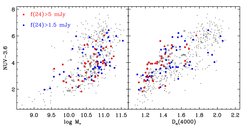
Figure 1: NUV-3.6 µm flux vs. log M_∗ (left) and D_n(4000) (right) for the SSGSS sample (solid circles). The blue circles are galaxies with 1.5 mJy $<$ F${}_{24~{}\micron}<5$ mJy and are observed with only low-res spectroscopy, while the red circles have F${}_{24~{}\micron}>1.5$ mJy and are observed with both low-res and hi-res modules. Unfilled circles are galaxies above the flux and surface brightness cuts but rejected due to high source density in those regions of parameter space. Black points are galaxies of the Lockman Hole sample (Johnson et al., 2006), the parent sample of SSGSS. Stellar masses are from Brinchmann et al. (2004).

MIR line ratios provide valuable diagnostics of HII regions. Electron densities can be studied using S III]${}_{18.7~{}\micron}$/[S III]${}_{33.4~{}\micron}$ and [Ne III]${}_{15.5~{}\micron}$/[Ne III]${}_{36.0~{}\micron}$, while ionization ratios can be studied using [Ne III]/[Ne II], [S IV]/[S III] and [Ar III]/[Ar II], and elemental abundances using various optical and MIR line species.

Many high stellar mass galaxies (log $M_{*}>10$) in the local universe and at z=1 possess composite optical emission-line spectra showing evidence of excitation by both young stars and AGN. These signatures are degenerate and are necessarily incomplete in characterizing reddened AGN. MIR ionization indicators such as [Ne III]/[Ne II] are invaluable for decomposing star formation and AGN emission because of the minimal levels of attenuation seen at these wavelengths (Weedman et al., 2006). Comparison of these with other AGN indicators, such as UV/optical line ratios (Kewley et al., 2001; Kauffmann et al., 2003b), and even PAH equivalent widths (EWs), allow us to analyse the diagnostic power of all of these measures. Combined with detailed MIR spectra, we can investigate the relative effects of AGN-sourced and starburst-sourced hard radiation fields on the ISM.

The abundance and composition of raw materials probably has a significant effect on the build-up and behaviour of dust grains. To better understand this effect, MIR abundance indicators combined with optical measures of gas-phase metallicity (Tremonti et al., 2004) can be compared with PAH bands, thermal dust continuum emission, and with MIR silicate absorption.

The molecular hydrogen IR fluorescence spectrum provides an indication of the physical conditions in photo-dissociation regions around molecular clouds and, while linked to the FUV radiation field, may also be produced by shocks in these regions.

3 Sample Definition and Properties

The SSGSS sample consists of 100 star-forming galaxies observed with Spitzer IRS in the Lockman Hole region, and is selected to have ancillary multi-wavelength imaging and spectroscopy from the FUV to the FIR, and to include galaxies with SFRs spanning the full range observed in the normal, star-forming population, short of the most extreme starbursting sources.

3.1 The Lockman Hole

The Lockman Hole, situated around $\alpha=10^{h}.7$, $\delta=50\deg$, is a $\sim$10 square degree field with one of the lowest column densities of interstellar material in the Milky Way, with $N_{HI}<7\times 10^{19}$, approximately 5% of the Galactic median. This makes it ideal for low-surface brightness surveys, and so it has been the subject of extensive multi-wavelength surveys. These include deep ROSAT imaging, deep GALEX (m_FUV,NUV 24.5 AB), SDSS imaging (m${}_{r}\sim 22.2$ AB) and spectroscopy, Deep 2MASS ($\times 6$, m${}_{K}\sim$17.8 AB, Beichman et al. 2003) and Spitzer/SWIRE (Lonsdale et al., 2003) IRAC (m $\sim$22.5, 20 for 3.6, 8.0 µm) surveys, as well as future programs (e.g. UKIDSS deep survey over the full region). The SDSS primary spectroscopic sample targets all galaxies with $r<17.8$ and yields $\sim 100$ galaxies deg^-1.

3.2 Selection Criteria

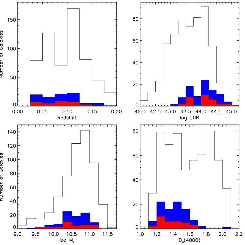
Figure 2: Distribution of SDSS-measured redshift, $L_{TIR}$, stellar mass, and D_n(4000) for SSGSS galaxies. The blue histograms show the 101 galaxies of the entire SSGSS sample, red histograms show the 33 galaxies of the SSGSS bright sample, and open histograms show the galaxies of the Lockman Hole sample of Johnson et al. (2006).

The Lockman Hole sample of Johnson et al. (2006) forms the parent sample for SSGSS, and consists of 916 galaxies at $z<0.2$ with GALEX-SDSS-Spitzer/SWIRE all-band coverage. The wide spectral coverage of this sample—from FUV to FIR—allows a consistent treatment of dust absorption and the corresponding dust emission, providing a total accounting of the star formation, stellar mass, and dust attenuation for these galaxies. A detailed description of these and other derived measurements and physical parameters can be found in Section 8.2. SSGSS targets a subset of this Lockman Hole sample for observation with the Spitzer IRS. These galaxies are selected based on two brightness criteria:

• 5.8 µm surface brightness: Galaxies fill the IRS Short-Low slit, and so at short-wavelengths we apply a surface brightness limit of I${}_{5.8\mu m}>0.75$ MJy sr^-1, based on IRAC 5.8 µm  flux and half-light diameter (the median/mean half-light diameter is 5Å for the entire sample).

• 24 µm  flux: At long wavelengths most of the galaxies are unresolved, and so a flux limit of F${}_{24\mu m}>1.5$ mJy is applied.

The above criteria yield 154 galaxies. We further restrict the sample by performing an even sampling of the planes of near-UV (NUV)-3.6 µm vs. stellar mass (from Brinchmann et al. 2004) and NUV-3.6 µm vs. $D_{n}(4000)$; in the dense regions of these spaces, we select the galaxy with the highest 24 µm flux. This process ensures that the sample spans a comprehensive range of physical properties. Figure 1 shows the distributions of NUV-3.6 µm color versus stellar mass and $D_{n}(4000)$ for the SSGSS galaxies compared to the Lockman Hole sample, and illustrates that the two span a similar range of galaxy properties. The Lockman Hole sample itself is representative of the SDSS galaxy sample with GALEX FUV detections; that is to say, normal, star-forming galaxies, consisting of both early- and late-type,s with $1.1\lesssim D_{n}(4000)\lesssim 2.1$.

The sample observed with Spitzer consists of 101 galaxies. Due to a fault with the SL spectrum for SSGSS 40, the current SSGSS data release consists of 100 galaxies. We preserve theoriginal indexing for consistency.

Within the SSGSS sample, we designate the bright sample and the faint sample, with the bright sample consisting of the 33 galaxies with F${}_{24\mu m}>5$ mJy. The entire sample is the subject of low-resolution 5 µm–40 µm IRS spectroscopy, while the bright sample is also observed with 10-20 µm high-resolution spectroscopy.

3.3 Sample Properties

This final SSGSS sample has a redshift range of $0.03<z<0.2$ with median redshift 0.085, and a total infrared luminosity ($L_{TIR}$) range of $3.7\times 10^{9}L_{\odot}<L_{TIR}<3.2\times 10^{11}L_{\odot}$, with median $3.9\times 10^{10}L_{\odot}$. The bright sample has redshift range of $0.04<z<0.2$ with median redshift 0.077, and an $L_{TIR}$ range of $5.1\times 10^{9}L_{\odot}<L_{TIR}<1.9\times 10^{10}L_{\odot}$ with median $6.9\times 10^{10}L_{\odot}$. The flux and surface brightness cuts do eliminate galaxies with very low stellar masses ($2\times 10^{9}M_{\odot}\leq M\leq 2\times 10^{11}M_{\odot}$), metallicities ($8.7\leq log(O/H)+12\leq 9.2$), and extinctions ($0.4<A_{H\alpha}<2.3$).

Table 1 details the 101 galaxies in the original SSGSS sample, and Figure 2 shows the distribution of redshift, stellar mass, $L_{TIR}$, and $D_{n}(4000)$ of the sample.

Table 1:

SSGSS	RA	DEC	z	NUV	r	LTIR (L⊙)	M∗ (M⊙)a	D${}_{n}(4000)^{b}$	S/Nc	Ap.Cor.d	Notes
1	160.34398	58.89201	0.066	18.04	16.22	3.90E+10	1.06E+10	1.14	17.1	-0.36	1
2	159.86748	58.79165	0.045	19.56	17.21	7.49E+09	3.67E+09	1.21	1.3	-0.37	1
3	162.41000	59.58426	0.117	22.42	17.17	4.21E+10	1.15E+11	1.57	10.6	-0.33
4	162.54131	59.50806	0.066	19.92	16.92	1.85E+10	1.74E+10	1.43	…	-0.90
5	162.36443	59.54812	0.217	20.94	17.71	2.64E+11	1.20E+11	1.28	10.8	-0.35
6	162.52991	59.54828	0.115	20.01	17.03	1.10E+11	8.50E+10	1.31	14.6	-0.59
7	161.78737	59.63707	0.090	20.35	17.17	2.76E+10	2.86E+10	1.42	7.4	-0.81	2
8	161.48123	59.15443	0.044	18.52	15.79	1.05E+10	2.88E+10	1.57	12.0	-1.15
9	161.59111	59.73368	0.121	20.79	17.23	5.33E+10	7.45E+10	1.42	12.3	-0.56	2
10	161.11412	59.74155	0.117	21.02	17.12	5.62E+10	8.59E+10	1.43	6.3	-0.50
11	161.71980	56.25187	0.047	20.14	16.44	5.85E+09	1.14E+10	1.46	5.9	-0.25	1
12	162.26756	56.22390	0.072	20.34	16.26	7.33E+10	1.20E+11	1.64	26.8	-0.41	1
13	163.00845	56.55043	0.124	20.96	17.46	4.31E+10	6.57E+10	1.49	15.5	-0.51
14	161.92709	56.31395	0.153	19.74	16.94	1.29E+11	7.32E+10	1.28	11.0	-0.37	1
15	161.75783	56.30670	0.153	21.13	17.56	1.93E+11	6.85E+10	1.41	33.9	-0.30	1
16	162.04231	56.38041	0.072	20.07	16.82	2.91E+10	2.87E+10	1.46	12.7	-0.31	1
17	161.76901	56.34029	0.047	20.65	16.00	7.43E+10	5.86E+10	1.37	33.9	-0.23	1
18	163.39658	56.74202	0.128	20.43	17.76	3.24E+11	4.27E+10	1.35	30.8	-0.58
19	163.44330	56.73859	0.076	19.07	16.41	3.31E+10	3.30E+10	1.27	4.1	-1.01	2
20	163.26968	56.55812	0.070	20.87	16.76	3.29E+10	3.57E+10	1.45	21.8	-0.29	3
21	163.19810	56.48840	0.077	19.77	16.28	3.17E+10	9.41E+10	1.64	5.1	-0.88	2
22	163.09050	56.50836	0.045	20.07	16.35	9.86E+09	1.89E+10	1.32	5.1	-0.52	2, 3
23	163.47926	56.44407	0.046	21.42	16.54	3.66E+09	1.60E+10	1.60	…	…	3
24	163.53931	56.82104	0.046	17.65	15.26	4.27E+10	2.50E+10	1.29	14.5	-0.95	2, 3
25	158.22482	58.10917	0.073	19.27	16.89	2.24E+10	1.16E+10	1.24	8.9	-0.74	3
26	159.04880	57.72258	0.093	19.65	16.46	2.89E+10	5.75E+10	1.50	9.7	-0.57
27	159.34668	57.52069	0.072	19.18	16.06	1.15E+11	4.04E+10	1.33	31.6	-0.55	1
28	158.91122	57.59536	0.103	21.54	17.15	8.89E+10	1.01E+11	1.77	16.5	-0.76	1, 2
29	158.91344	57.71219	0.113	19.88	16.50	4.22E+10	1.14E+11	1.47	6.7	-0.85
30	159.73558	57.26361	0.046	19.99	17.39	1.42E+10	3.84E+09	1.22	15.3	-0.23	1
31	159.63510	57.40035	0.047	18.70	15.41	7.99E+09	4.90E+10	1.72	10.4	-1.26
32	161.48724	57.45520	0.117	19.96	17.59	7.23E+10	2.47E+10	1.15	13.5	-0.20	1
33	160.29099	56.93161	0.185	20.76	17.13	1.92E+11	1.68E+11	1.38	19.1	-0.34	1
34	160.30701	57.08246	0.046	20.35	17.05	1.01E+10	6.62E+09	1.22	7.5	-0.21	1
35	160.31664	56.89586	0.185	20.33	17.69	3.19E+11	1.06E+11	1.24	…	…	1
36	159.98523	57.40522	0.072	19.53	16.55	2.76E+10	3.74E+10	1.36	9.9	-0.73
37	160.10915	57.43977	0.047	19.86	15.61	1.40E+10	5.65E+10	1.68	11.9	-1.01
38	160.20963	57.39475	0.118	20.07	16.92	9.40E+10	6.77E+10	1.28	17.4	-0.60
39	159.38356	57.38491	0.074	19.81	17.35	1.57E+10	1.04E+10	1.27	6.5	-0.30	1
40	159.79688	57.27135	0.102	20.55	17.00	4.61E+10	1.09E+11	1.39	…	…
41	158.99098	57.41671	0.102	21.03	17.28	2.46E+10	5.96E+10	1.48	6.5	-0.49
42	158.97563	58.31007	0.155	19.80	17.31	1.18E+11	9.13E+10	1.36	10.2	-0.58
43	158.85551	58.28600	0.114	20.14	17.22	4.76E+10	4.82E+10	1.35	10.5	-0.60
44	159.74423	58.37608	0.068	20.00	16.58	5.44E+10	3.52E+10	1.39	…	…
45	159.06448	57.65416	0.113	21.24	17.12	4.79E+10	8.44E+10	1.50	6.4	-0.54	1
46	159.02698	57.78402	0.044	19.06	17.05	1.17E+10	7.09E+09	1.20	14.7	-0.61
47	159.22287	57.91185	0.102	19.89	17.42	5.33E+10	1.88E+10	1.17	7.9	-0.50	1
48	159.98817	58.65948	0.200	20.07	17.69	1.95E+11	6.50E+10	1.21	9.0	-0.26	1
49	159.51942	58.04882	0.091	19.10	16.82	3.47E+10	2.77E+10	1.18	12.7	-0.72
50	159.78503	58.23109	0.073	19.45	16.02	1.65E+10	7.10E+10	1.76	…	…
51	159.85828	57.96801	0.138	20.21	17.13	9.76E+10	1.14E+11	1.38	10.0	-0.46
52	160.54201	58.66098	0.031	19.33	16.26	3.82E+09	7.10E+09	1.43	5.4	-0.80	2
53	160.57785	58.68312	0.120	19.99	16.54	4.48E+10	1.22E+11	1.66	5.2	-0.95	2
54	160.41264	58.58743	0.115	20.73	16.98	1.78E+11	1.59E+11	1.41	19.2	-0.45	1
55	160.29353	58.25641	0.121	20.38	17.41	3.86E+10	4.01E+10	1.38	6.6	-0.60
56	160.41617	58.31722	0.072	21.58	15.80	1.11E+10	1.36E+11	1.90	8.2	-0.56
57	160.12233	58.16783	0.073	20.88	17.02	9.20E+09	2.62E+10	1.46	…	…
58	160.10104	58.15516	0.072	…	16.74	3.49E+10	6.44E+10	1.65	…	…
59	159.89861	57.98557	0.075	20.10	16.55	2.55E+10	5.13E+10	1.50	10.8	-0.32
60	160.51027	57.89706	0.116	20.24	17.13	3.30E+10	6.96E+10	1.47	8.6	-0.53
61	160.95200	58.19655	0.073	20.48	16.48	2.19E+10	5.19E+10	1.42	10.1	-0.34	1
62	160.91280	58.04736	0.133	19.47	17.14	1.34E+11	6.03E+10	1.23	16.8	-0.51	1
63	160.88481	57.67214	0.046	20.10	14.50	3.71E+09	1.00E+00	2.03	1.3	-0.68	2
64	161.00317	58.76030	0.073	20.42	16.59	8.43E+10	9.93E+10	1.49	20.2	-0.58	1
65	161.37666	58.20886	0.118	19.99	16.48	1.67E+11	1.99E+11	1.38	21.8	-0.39	1
66	161.25533	57.77575	0.113	19.93	17.42	7.82E+10	5.31E+10	1.30	13.1	-0.36
67	161.18829	58.45495	0.031	0.00	14.46	1.34E+10	1.00E+00	1.50	25.6	-1.39
68	163.63458	57.15902	0.068	19.95	15.94	3.79E+10	6.40E+10	1.46	18.0	-0.28
69	162.27214	57.62591	0.076	20.23	17.22	3.28E+10	2.91E+10	1.41	8.9	-0.26	1
70	163.17673	57.32074	0.090	20.54	17.73	3.34E+10	1.82E+10	1.26	5.0	-0.15	1
71	163.21991	57.13160	0.163	21.46	17.59	1.03E+11	1.08E+11	1.46	7.5	-0.38
72	163.25565	57.09528	0.080	19.97	17.06	6.88E+10	3.01E+10	1.26	19.1	-0.35
73	163.35274	57.20859	0.080	20.35	17.38	1.29E+10	1.77E+10	1.38	4.0	-0.35	1
74	161.95050	57.57723	0.118	19.88	17.01	6.98E+10	5.49E+10	1.24	15.2	-0.63
75	162.14607	58.02331	0.176	20.28	17.28	9.75E+10	2.14E+11	1.48	…	-0.71
76	162.02142	57.81512	0.074	20.35	17.60	4.05E+10	2.49E+10	1.23	6.9	-0.51
77	162.10524	57.66665	0.044	19.20	17.37	5.35E+09	1.98E+09	1.13	4.8	-0.27	1
78	162.12204	57.89890	0.074	18.71	16.21	4.10E+10	3.08E+10	1.28	13.7	-0.87	2
79	161.25693	57.66116	0.045	19.00	16.48	7.28E+09	8.57E+09	1.28	4.2	-0.97
80	162.07401	57.40280	0.075	18.67	16.81	2.50E+10	2.97E+10	1.29	8.2	-0.82
81	162.04674	57.40856	0.075	19.63	17.12	1.91E+10	1.67E+10	1.38	6.1	-0.60
82	161.03609	57.86136	0.121	20.11	17.14	6.62E+10	5.52E+10	1.22	6.7	-0.53
83	160.77402	58.69774	0.119	19.73	17.13	9.17E+10	4.23E+10	1.29	16.0	-0.69	1
84	162.48495	59.50835	0.116	22.19	17.29	4.78E+10	1.32E+11	1.74	6.2	-0.74	2
85	162.13954	59.01889	0.063	21.31	17.36	6.96E+09	2.07E+10	1.59	5.1	-0.42
86	162.01674	58.86004	0.085	19.25	16.24	2.86E+10	7.62E+10	1.55	4.8	-1.01
87	161.40736	58.19447	0.116	20.37	16.79	2.55E+10	8.54E+10	1.49	3.8	-0.71	2
88	161.38522	58.50156	0.116	20.89	17.41	3.59E+10	4.11E+10	1.40	5.1	-0.34
89	161.55003	58.44921	0.050	19.21	15.61	7.08E+09	4.94E+10	1.68	6.2	-1.84	2
90	162.64168	59.37266	0.153	20.19	17.54	1.16E+11	5.32E+10	1.26	17.4	-0.26
91	162.53705	58.92866	0.117	19.07	16.75	6.80E+10	5.44E+10	1.21	8.2	-0.85
92	162.65512	59.09582	0.032	18.20	15.51	1.64E+10	1.08E+10	1.22	34.9	-0.59
93	162.79474	59.07684	0.117	22.42	17.36	4.42E+10	8.82E+10	1.63	9.2	-0.29
94	161.80573	58.17759	0.061	21.47	17.70	1.52E+10	1.30E+10	1.42	3.8	-0.39	1
95	163.71245	58.39082	0.115	20.79	17.39	7.16E+10	6.38E+10	1.33	14.5	-0.25	1
96	164.74986	58.25686	0.132	20.42	17.39	6.45E+10	6.72E+10	1.40	9.0	-0.29	2
97	164.77032	58.32224	0.131	19.93	17.15	7.41E+10	8.82E+10	1.32	7.4	-0.71	2
98	164.14571	58.79676	0.050	18.18	16.31	4.28E+10	8.34E+09	1.13	24.8	-0.56	1
99	164.33247	57.95170	0.077	18.56	16.42	7.35E+10	1.88E+10	1.19	20.2	-0.67	1
100	164.74155	58.13369	0.032	20.26	15.39	5.45E+09	3.32E+10	1.66	9.2	-0.95	2
101	164.46204	58.23759	0.077	21.69	16.93	1.21E+10	1.95E+10	1.54	11.0	-0.20	2
Notes
1. Bright sample target; observed with SH module
2. Problematic calibration of SL2 module
3. Affected by solar flare
a. Stellar mass from Kauffmann et al. (2003a)
b. $D_{n}(4000)$ from Kauffmann et al. (2003a)
c. Signal-to-noise ratio of SSGSS low resolution spectra at 22 µm (see Sect. 5.3)
d. IRAC 7.8 µm mag minus synthetic 7.8 µm mag for aperture correction of SL module (see Sect. 5.4)

4 New Spitzer Spectroscopy

4.1 Instrument, Observing Mode, and AORs

The full SSGSS sample was observed with the IRS on board the Spitzer Space Telescope as a Cycle-3 Legacy Survey. All spectroscopic observations were performed in spectral mapping mode. Observations were divided between 29 Astronomical Observation Requests (AORs), each consisting of 4 to 8 galaxies observed in cluster mode. All galaxies within an AOR were observed consecutively, using guided telescope shifts to move between targets.

4.2 Low-Resolution IRS Spectroscopy

The entire SSGSS sample was observed with the IRS ‘low-res’ Short-Low (SL) and Long-Low (LL) modules. The SL module spans 5.2 to 14.5 µm  with resolving power $R=60$–125 and has slit width 3$\farcs$6–3$\farcs$7. The LL module spans 14 to 38 µm  with resolving power $R=57$–126 and has slit width 10$\farcs$5–10$\farcs$7. Both the SL and LL modules are divided into two sub-slits—the first and second orders—abbreviated SL1 (7.4-15.4 µm), SL1 (5.2-8.7 µm), LL1 (19.5-38 µm), and LL2 (14.0-21.3 µm). Telescope shifts position the source over each order, and so the first and second orders appears on opposite halves of the detector. A third, ‘bonus’ order from an additional sub-slit is obtained with the second order.

Four offsets in the direction of the slit were used to produce a 1-D dither pattern, with two exposures at each position. This strategy has been shown to increase the quality of output spectra, in particular for the handling of rogue pixels, undersampling, and flat-fielding as described in the IRS instrument support team document Obtaining Spectra of Very Faint Sources with the IRS, and in Teplitz et al. (2007).

For low-res spectroscopy our sensitivity target was 5$\sigma$ per resolution element for the continuum and PAH band features, after moderate smoothing for the faintest sources. To achieve this sensitivity, our bright-sample exposure times are 8 minutes in both the SL and LL modules and our faint-sample exposure times are 8 minutes in the SL and 16 minutes in the LL module.

4.3 High-Resolution IRS Spectroscopy

The 33 galaxies in the SSGSS bright sample were also observed with the IRS ‘hi-res’ Short-High (SH) module. This module spans 9.9 to 19.6 µm  with $R\approx 600$, and has slit width 4$\farcs$7.

For the hi-res spectroscopy our target line flux was $1\times 10^{-18}$ W m^-2 at 5$\sigma$, based on the line fluxes for [Ne II], [Ne III], [Ar II] and [S III] for star-forming galaxies with infrared luminosities comparable to those in the bright sample. Our hi-res exposure times are 16 minutes, split over separate exposures.

For each hi-res AOR, eight separate sky spectra with a total of 16 minute exposure times were also taken.

4.4 Slit Positions

A crucial aspect of this program is the comparison of MIR spectral properties to SDSS optical properties and so it was essential to ensure overlap between the slit and the 3″ SDSS fiber. All slits are wider than the SDSS aperture, and so the SDSS aperture was centered within each slit with at least 0$\farcs$5 accuracy. Acquisition (“peak-up”) imaging at each AOR enabled us to achieve this accuracy, as descrived in Section 4.5.

Slit orientations were not specified and so are random. As the SL and LL observations are taken consecutively, the relative orientation of these slits on each galaxy is the same as their relative orientation on the spacecraft ($85.9^{\circ}$). SH slit positions are randomly oriented with respect to the low-res positions.

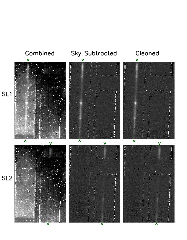
Figure 3: Example SL1 (upper) and SL2 (lower) frames through the reduction process. Left is the post-pipeline combined frame, middle is the sky-subtracted frame, and right is the cleaned sky-subtracted frame, from which 1-D spectra are extracted. Pointers mark the ends of the spectra—to the left of the frames for SL1, and to the lower right for SL2. The segments at the upper right are the bonus order spectra.

4.5 Peak-up Imaging

To achieve the accuracy needed for our slit positioning, we preceeded the observations in each AOR with a pointing-mode peak-up image. The IRS Peak-Up facility uses centroid positioning from an image of the field in the SL detector array to position the science target in the slit. In our case, we used bright sources with known offsets to the targets. Despite the high galactic latitude of our sources, there were sufficient bright, low-proper-motion sources in each field to ensure quality peak-ups.

In addition, each galaxy was observed with dedicated 4$\times$30 second peak-up imaging. These peak-ups utilized the blue filter, with spectral coverage of 13.3–18.7 µm. This $\sim 16$ µm coverage gives us photometric data intermediate to the IRAC 8 µm  and MIPS 24 µm  imaging.

Figure 18 (Appendix A) shows the dedicated peak-up images for all galaxies in the sample, including slit positioning.

4.6 Solar Flare

A solar flare during one AOR resulted in very high cosmic ray counts for five targets. The affected galaxies are SSGSS 20, 22, 23, 24, and 25.

5 Data Reduction

5.1 Low-Resolution Spectroscopy

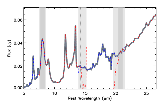
Figure 4: Example of method used to stitch the low-res spectra. The colored dashed spectra are from individual channels, from left to right: SL2 (blue), SL1 (red), LL2 (blue), LL1 (red). The dark gray spectrum is stitched from these channels. Dark gray shaded areas represent the channel-overlap regions where two channels are medium-combined. The light gray shaded areas are the channel-overlap regions where the stitched spectrum is set to the values of the nearest channel. The default medium-combined region is the central 50% of the overlap region, however this is adjusted manually to avoid end-of-channel transmission drops. The dotted line is the stitch point for the SL1–LL2 junction, which defaults to the middle of the overlap region but in many cases is set manually due to transmission drops.

Standard IRS processing was performed by the Spitzer Pipeline version S15.3.0. Pipeline steps included ramp fitting, dark subtraction, droop, linearity correction and distortion correction, flat fielding, masking and interpolation, and wavelength calibration.

No separate sky images were taken with the low-res modules and so sky frames were constructed from combined science frames. Between the first- and second-order exposures, the source is shifted to opposite sides of the detector. This results in a sky exposure for the order not currently containing the source. Within each AOR, all such sky exposures were median combined to produce a master sky frame for each order.

Bad and rogue pixels masks for each exposure were created with IRSCLEAN (version 1.9), with AGGRESSIVE keyword set to 2, and with negative pixels also masked. We also applied the campaign rogue pixel masks released by Spitzer.

Figure 3 shows example frames for the SL module through the reduction process, including the initial post-pipeline frame with exposures combined, the sky-subtracted frame, and the cleaned frame.

Extraction of 1-D spectra was performed using SPICE version 2.0.1. The default setting was used to create a wavelength collapsed spatial profile, and the center of the profile was determined manually due to excess failures of the auto-center option. SPICE then performed spectral extraction along this peak. The point source tune module applied flux corrections for changes in the wavelength-dependent Point Spread Function (PSF) width and aperture size, and assumed emission by a point source.

5.1.1 Low-res Combining and Stitching

The extracted 1-D spectra were combined by weighted mean. First, the spectra at the four dither positions along the slit were were combined for each order. Then the first, second and bonus orders were stitched to produce separate SL and LL spectra using the following semi-manual process: by default, the central 50% of each overlap region was combined by weighted mean and the outer quartiles of the overlap region were set to the nearest order. In select cases the combined region was adjusted to avoid obvious drops in transmission at the ends of either order. The SL and LL modules were combined by a clean cut between the spectra, determined manually to avoid end-of-channel transmission drops. Figure 4 illustrates the method used for stitching spectra.

The overlap region of the SL and LL modules is $\sim 14$–$14.5$ µm, and in this region the slit widths are 3$\farcs$7 and 10$\farcs$5 for SL and LL respectively. The approximate LL-to-SL ratio of admitted light from centrally-aligned point source in the overlap region is $\sim$1.3, based on a simple model of the Spitzer PSF (Smith, 2004), and the overall LL sensitivity is a factor of $\sim$5 higher than the SL module in this region (Spitzer Observer’s Manual, p.160). While these differences are accounted for by the pipeline reduction assuming a centrally-aligned point source, for extended sources we may expect an offset at their intersection when the spectra are stitched.

In fact no galaxies exhibit noticeable discontinuities across the modules in this region, indicating that deviations from the point-source approximation in the overlap region are small, even for the SL module at $\sim$14–15µm. No re-scaling was necessary or performed.

5.2 High-Resolution Spectroscopy

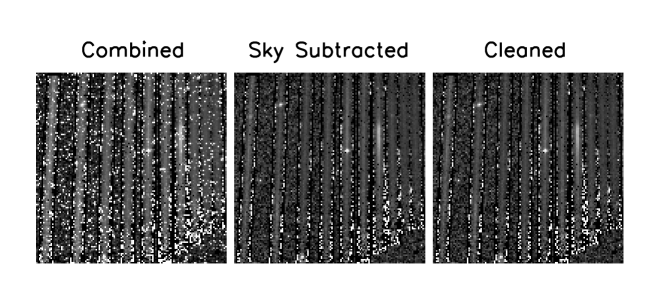
Figure 5: Example SH frames through the reduction process. Left is the post-pipeline combined frame, middle is the sky-subtracted frame, and right is the cleaned sky-subtracted frame, from which 1-D spectra are extracted.

As with the low-resolution spectroscopy (Sect. 5.1), the Spitzer Pipeline version S15.3.0 was used to perform standard IRS processing. Unlike the low-res data, for the hi-res observations we combined the eight separate exposures of each galaxy before extraction. This improved the signal to allow higher quality extractions.

As noted in Section 4.3, separate hi-res sky frames were taken for each AOR, median combined from eight 16 minute exposures. Masking followed the same method used for the low-res spectroscopy, utilizing IRSCLEAN (version 1.9) and the Spitzer campaign rogue pixel mask. Likewise, extraction was performed as for the low-res data, using SPICE v.2.0.1. The hi-res orders were stitched into a single spectrum using a similar method to the low-res spectra: order-overlap regions were combined by taking the weighted mean within the central 50% or the overlap regions, while for the outer quartiles the nearest order was used.

Figure 5 shows example frames for the SH module through the reduction process, including the initial post-pipeline frame with exposures combined, the sky-subtracted frame, and the cleaned frame.

5.3 Achieved Sensitivity

Figure 6: Signal-to-noise ratios of low-res spectra at 10 µm (upper) and 22 µm (middle) versus IRAC 7.8 µm and MIPS 24 µm mag respectively, and of the hi-res spectra at 15 µm versus MIPS 24 µm mag. Dashed lines indicate target S/N.

Figure 7: Signal-to-noise ratios of the [Ne II] (upper) and [Ne III] (lower) emission lines from the hi-res spectra versus the PAHFIT-measured fluxes. Dashed lines indicate target S/N.

We estimate the continuum sensitivity achieved by determining the signal-to-noise ratio (S/N) in the processed spectra at relatively featureless regions of the spectra. We compare the mean flux to the corresponding noise in the regions 9–10 µm and 20–24 µm for the low-res spectra and 14.7–15.3 µm for the hi-res spectra. The noise is taken to be the standard deviation in these regions after subraction of a power law fit. Figure 6 shows the continuum S/N for low-res and hi-res spectra versus IRAC 7.8 µm and MIPS 24 µm mag. At $\sim 22$ µm nearly all sources exceed the target S/N $=$ 5, with a minimum S/N of 4, and have the expected tight relationship with 24 µm mag. At $\sim 10$ µm the variable silicate absorption results in a number of sources with S/N $<$ 5. In this case there is greater variability of S/N with photometric magnitude due to this absorption and the overlap of more PAH bands with the IRAC 7.8 µm band. 22 µm S/N is provided in Table 1.

We estimate the S/N for the [Ne II]_12.8 and [Ne III]_15.6 emission lines in the hi-res spectra by comparing the integrated flux of the lines to the standard deviation in the relatively smooth, blueward regions at 12.25–12.75 µm and 15–15.5 µm. Figure 7 shows line S/N versus the line flux (see Sect. 6.3). [Ne II] and [Ne III] are detected in all galaxies with S/N $>$ 5. In most cases, both [Ne II] and [Ne III] are detected with S/N $>$ 10. There is strong scatter in the trend between line flux and S/N due to the weakness of the trend between continuum and line luminosity, and this is especially pronounced in [Ne III], where the line emission may be linked more to an AGN components than to star formation.

The flux uncertainties reported by SPICE, which are included in the released data, have been checked for the low-res modules by comparing the multiple dithered observations for each galaxy. These uncertainties were found to be accurate to within a factor of 1.5.

5.4 Aperture Effects

Figure 8: Synthetic minus SWIRE photometry as a function of r-band petrosian radius 8 µm, 16 µm, 24 µm. The trend between this magnitude difference and radius observed in the 8 µm band suggests slit losses in the SL module, but not at longer wavelengths.

Figure 9: SL slit aperture magnitude minus synthesized and circular aperture magnitudes as a function of r band petrosian radius.

An increasing fraction of the wavelength-dependent Spitzer PSF falls outside a given IRS slit with increasing wavelength. The standard spectral extraction with SPICE corrects for this slit loss assuming emission by a point source. At $>$ 16 µm the combination of the larger Spitzer PSF and the wider IRS slits means that all galaxies are well-approximated as point sources (Fig. 18, Appendix A). However, a number of the SSGSS galaxies have sufficient spatial extent that they are not well-approximated by point sources in the narrower SL and SH modules.

We investigate slit loss in the low resolution modules by comparing synthetic photometry from the reduced, calibrated low-res spectra to large-aperture photometry obtained from SWIRE imaging (IRAC channel 4 7.8 µm and MIPS 24 µm), and from the SSGSS 16 µm peak-up imaging. Synthetic photometry is obtained by integrating the spectra using k_correct (v4.14; Blanton03b). Figure 8 shows the difference in these magnitudes as a function of the $r^{\prime}$ band Petrosian radius ($R_{P}$), with aperture photometry performed in 7″ and 12″ radius apertures for 8 µm and 24 µm respectively, as described in Johnson et al. (2007). Differences may be attributed to a number of sources (e.g., source confusion in the imaging aperture photometry, relative calibration errors) but any trend with the angular size of the galaxy is suggestive of slit losses. No such trend is observed at 16 µm and 24 µm. However, at 8 µm a significant trend is apparent, indicating slit losses in the SL module.

To isolate the effect of slit loss from any calibration uncertainties, we perform photometry of the 8 µm IRAC images within the region corresponding to the SL slit aperture (a 3$\farcs$65$\times$9$\farcs$6 rectangle), and compare this to the synthetic and circular aperture magnitudes. Figure 9 (upper) shows the difference between slit aperture and synthetic magnitudes. A 0.3 mag aperture correction is applied by SPICE at 8 µm and so the synthetic magnitudes are higher than the derived slit aperture magnitudes. Taking this offset into account, the slit aperture samples more flux than the extracted spectra, with an average offset of $\sim 0.2$ mag and similar scatter. The magnitude difference is independent of galaxy size, indicating that the trend observed in Figure 8 does not result from calibration effects. Figure 9 (lower) shows slit aperture versus circular aperture magnitudes, revealing a similar trend to that observed with the 8 µm synthetic magnitudes. The maximum difference is 1-1.5 mag for $R_{p}(r^{\prime})\gtrsim 9\arcsec$,

The apparent slit losses in the SL module mean that care is necessary when considering the shape of the ($\lesssim 16~{}\micron$) Spectra Energy Distribution (SED) of large galaxies. The difference between the synthetic and photometric magnitudes at 8 µm should provide a reasonable estimate of the aperture correction. These corrections are provided Table 1.

6 SSGSS Data

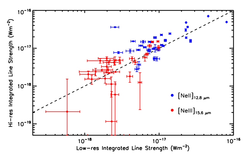
Figure 10: Comparison of the [Ne II]_12.8 µm (blue) and [Ne III]_15.6 µm (red) emission line integrated strengths as measured with PAHFIT using the low-res and hi-res spectra. Error bars represent the 1-$\sigma$ uncertainties in the fits.

Figure 18 shows multi-wavelength imaging for all 101 galaxies in the SSGSS sample, including GALEX FUV and NUV, SDSS multi-colour, r, H, IRAC 3.6 µm and 8 µm, 16 µm from SSGSS peakup images, and MIPS 25 µm and 70 µm. Overlaid are the slit positions for the SL, LL, and SH modules.

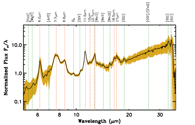
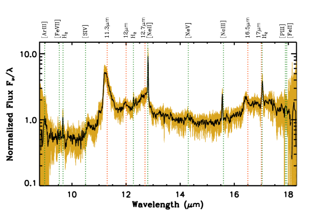
Figure 11: Upper panel: composite SL and LL low-res spectrum of the 100 galaxies of the current SSGSS data release (solid black line). Low-res spectra are normalized between 20–24 µm. The shaded region represents 1-sigma scatter of the normalized spectra about the mean spectrum. Lower panel: composite SH hi-res spectrum of the 33 galaxies of the SSGSS bright sample. Hi-res spectra are normalized between 14–15 µm.

6.1 Low-Resolution Spectra

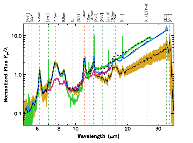
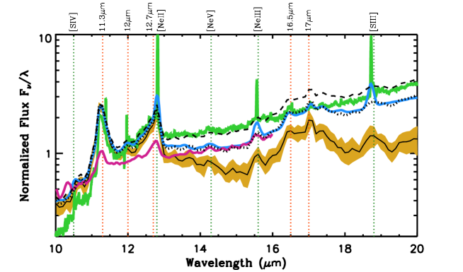
Figure 12: Top: Composite low-res spectrum of the SSGSS sample (solid black line), with the spectrum of M82 (green; Sturm et al 2000), the composite spectrum of local starbursts (blue; Brandl et al. 2006), and the composite of $z\sim 1$ ULIRGS (magenta; Dasyra et al. 2009). The shaded region represents the 1-sigma scatter of the normalized spectra about the mean spectrum. The dotted black lines show best fits to M82 and starburst composites of a model consisting of the SSGSS composite plus a dual-temperature blackbody. The fits indicate that starburst spectra are well represented by that of a normal, star-forming galaxy plus an enhanced thermal dust component at $T\lesssim 120K$. Bottom: 10–20µm region of top panel.

Figure 19 (Appendix B) shows the reduced, combined, and stitched SL and LL spectra for the 100 galaxies in the current data release. For each galaxy the SSGSS catalog number, BPT type (Baldwin et al., 1981; Kewley et al., 2001; Kauffmann et al., 2003b), redshift, stellar mass, NUV-R color, and $D_{n}(4000)$ are given.

The relatively low sensitivity of the 5.25–7.58 µm SL2 module, coupled with the relative faintness of many galaxies in this range, results in very low SL2 signal in 10 sources. This spectral region should be used with caution in these sources, which are noted in Table 1.

For one galaxy, SSGSS 56, the SL–LL overlap region falls directly on the redshifted 12µm PAH complex and the [Ne II]_12.8 line. End-of-order transmission drops in both the SL and LL modules affect these features, and so both are lost in this spectrum.

6.2 High-Resolution Spectra

Figure 20 (Appendix B) shows the reduced, combined, and stitched SH spectra for the 33 galaxies in the SSGSS bright sample. For each galaxy the SSGSS catalog number, BPT type, redshift, stellar mass, NUV-R color, and $D_{n}(4000)$ are given.

6.3 Emission Line Strengths

We measure emission line strengths by integrating line regions after subtraction of the continuum. Here, the continuum refers to all non-emission line features, including PAH features and the thermal continuum. The continuum is determined using the PAHFIT code of Smith et al. (2007), which fits a physically-motivated model to each spectrum using $\chi^{2}$ minimization. We describe our use of PAHFIT in detail in O’Dowd et al. (2009) (OD09). When applied to the hi-res spectra, we remove emission line fitting from the process and mask the emission line regions. We are not concerned with accurate measurement of continuum features—only that we find a reasonable extrapolation of the continuum in the region of the emission lines.

The emission line strengths measured by PAHFIT from the hi-res spectroscopy are highly reliable, as the continuum near most lines is reasonably smooth, allowing robust subtraction. These line strengths compare closely to those measured using a simple linear fit to the continuum surrounding each line. In the case of the [Ne II]_12.8 line, PAHFIT is significantly more reliable than cruder continuum-fitting methods because of the close proximity of this line to the peak of the 12.7 µm PAH feature.

Figure 10 compares [Ne II]_12.8 and [Ne III]_15.6 lines strengths between the low- and hi-res spectra. Although there is general agreement, on average the low-res spectroscopy shows weaker line strengths by $\sim$20–50%, with similar scatter compared to the hi-res spectra. In four galaxies, PAHFIT claims detection of [Ne III] lines in the low-res spectra where they are undetected at high resolution. The uncertainties reported by PAHFIT for the low-res [Ne II] lines are significantly underestimated, suggesting that there is more degeneracy between this line and the 12.6 µmPAH complex than estimated by in the fit.

Table 2 gives emission line strengths measured from the hi-res spectra. Line strengths from the low-res spectra can be found on the SSGSS website (see Sect. 8.2).

6.4 Composite Spectra

Table 2:

SSGSS	[S IV]10.5µm	[Ne II]12.8µm	[Ne III]15.6µm	H2 (9.7 µm)	H2 (12.2 µm)
1	1.71 $\pm$ 0.59	11.50 $\pm$ 0.41	1.25 $\pm$ 1.01	…	1.64 $\pm$ 0.55
2	1.89 $\pm$ 1.28	3.67 $\pm$ 0.79	4.79 $\pm$ 1.12	1.54 $\pm$ 0.62	0.97 $\pm$ 0.39
11	0.84 $\pm$ 0.91	2.80 $\pm$ 0.40	0.21 $\pm$ 1.32	2.82 $\pm$ 0.62	1.44 $\pm$ 0.49
12	3.58 $\pm$ 0.57	36.55 $\pm$ 0.42	4.20 $\pm$ 0.51	3.52 $\pm$ 0.89	4.90 $\pm$ 0.77
14	0.77 $\pm$ 0.48	12.15 $\pm$ 0.43	2.22 $\pm$ 0.00	3.88 $\pm$ 0.82	4.28 $\pm$ 1.21
15	…	9.65 $\pm$ 0.43	…	3.30 $\pm$ 0.78	1.40 $\pm$ 0.98
16	3.63 $\pm$ 0.47	14.50 $\pm$ 0.38	1.52 $\pm$ 0.41	1.13 $\pm$ 0.78	4.70 $\pm$ 0.77
17	4.27 $\pm$ 1.25	49.26 $\pm$ 0.43	11.58 $\pm$ 1.04	10.85 $\pm$ 0.62	9.81 $\pm$ 0.49
27	6.60 $\pm$ 0.51	70.46 $\pm$ 0.39	14.78 $\pm$ 0.47	3.99 $\pm$ 0.91	13.77 $\pm$ 0.82
28	…	8.47 $\pm$ 0.96	4.67 $\pm$ 0.63	6.14 $\pm$ 0.78	2.45 $\pm$ 0.33
30	2.57 $\pm$ 0.84	5.33 $\pm$ 0.61	4.84 $\pm$ 0.98	4.45 $\pm$ 0.71	1.24 $\pm$ 0.47
32	2.34 $\pm$ 0.65	10.22 $\pm$ 2.29	5.32 $\pm$ 0.63	2.67 $\pm$ 0.49	2.74 $\pm$ 0.52
33	5.15 $\pm$ 1.13	8.32 $\pm$ 1.21	2.64 $\pm$ 0.00	4.22 $\pm$ 0.53	…
34	3.28 $\pm$ 0.80	10.60 $\pm$ 0.42	3.28 $\pm$ 0.97	1.16 $\pm$ 0.73	2.55 $\pm$ 0.44
35	…	9.66 $\pm$ 0.43	…	3.35 $\pm$ 0.78	1.39 $\pm$ 0.98
39	…	9.04 $\pm$ 0.38	1.58 $\pm$ 0.39	…	…
45	…	19.16 $\pm$ 1.09	1.13 $\pm$ 0.62	1.29 $\pm$ 0.54	1.26 $\pm$ 0.37
47	…	16.12 $\pm$ 1.09	2.40 $\pm$ 0.53	1.71 $\pm$ 0.52	2.49 $\pm$ 0.33
48	…	9.01 $\pm$ 0.64	2.38 $\pm$ 0.00	1.03 $\pm$ 1.16	1.91 $\pm$ 0.48
54	4.60 $\pm$ 0.96	15.67 $\pm$ 1.42	1.81 $\pm$ 0.56	4.46 $\pm$ 0.52	4.61 $\pm$ 0.50
61	3.51 $\pm$ 0.58	36.07 $\pm$ 0.45	4.27 $\pm$ 0.55	3.62 $\pm$ 0.87	4.64 $\pm$ 0.76
62	3.93 $\pm$ 0.71	24.36 $\pm$ 0.53	…	4.31 $\pm$ 0.97	5.32 $\pm$ 0.81
64	3.84 $\pm$ 0.57	47.83 $\pm$ 0.46	6.96 $\pm$ 0.51	3.98 $\pm$ 0.73	7.26 $\pm$ 0.95
65	2.54 $\pm$ 0.70	30.40 $\pm$ 2.29	5.39 $\pm$ 0.57	4.46 $\pm$ 0.58	4.16 $\pm$ 0.42
69	…	14.81 $\pm$ 0.45	2.05 $\pm$ 0.44	1.03 $\pm$ 1.17	2.54 $\pm$ 0.82
70	1.08 $\pm$ 0.53	9.12 $\pm$ 0.63	2.68 $\pm$ 0.37	…	1.45 $\pm$ 0.43
73	1.33 $\pm$ 0.58	7.69 $\pm$ 0.48	…	4.64 $\pm$ 0.95	1.54 $\pm$ 0.53
77	4.99 $\pm$ 1.44	11.72 $\pm$ 0.41	5.70 $\pm$ 1.14	…	4.74 $\pm$ 0.38
83	…	5.25 $\pm$ 0.63	4.23 $\pm$ 0.68	5.20 $\pm$ 0.57	2.59 $\pm$ 0.50
94	1.85 $\pm$ 0.65	15.28 $\pm$ 0.33	0.60 $\pm$ 0.70	2.10 $\pm$ 0.64	2.59 $\pm$ 0.50
95	…	14.85 $\pm$ 1.16	0.12 $\pm$ 0.60	2.65 $\pm$ 0.66	2.17 $\pm$ 0.43
98	4.34 $\pm$ 1.33	19.02 $\pm$ 0.80	10.46 $\pm$ 1.35	5.25 $\pm$ 0.72	7.06 $\pm$ 0.64
99	4.71 $\pm$ 0.54	22.53 $\pm$ 0.41	15.16 $\pm$ 0.39	2.39 $\pm$ 1.26	…
Line fluxes in $10^{-18}$ Wm-2

Figure 11 (upper) shows the composite of the low-res SL and LL spectra for the entire SSGSS sample, normalized between 9–11 µm. Primary PAH features are prominent, including a pronounced 17 µm complex. Several emission lines are also distinct.

Figure 11 (lower) shows the composite of the SH spectra for the SSGSS bright sample, normalized between 14–15 µm. PAH features have significantly more detailed line profiles than in the low-res spectra, including clear resolution of the 16.5 µm feature from the 17 µm complex and interesting structure in both the 11.3 µm and 12.7 µm features. In addition, the [Ne III]_15.6µm line is well-resolved from the 12.7 µm feature.

7 Results and Discussion

7.1 Comparison to Starburst Spectra

The SSGSS sample spans the range of physical properties of ‘normal’ star-forming galaxies, as described in Section 3. We investigate the difference between the composite SSGSS spectra and galaxy spectra of previous IR surveys which have typically been dominated by more extreme starburst galaxies.

Figure 12 shows the low-res SSGSS composite spectrum (normalized between 9–11 µm for composite construction) overplotted with an ISO spectrum of M82 (Sturm et al, 2000) and the Spitzer local starburst composite of Brandl et al. (2006). These spectra are normalized according to the results of the fits described below. Also plotted is the $0.8<z<1.2$ LIRG composite of Dasyra et al. (2009), normalized at the blue end of this spectrum, 6.5-6.8 µm.

M82 and the local starburst composite have similar EWs for PAH features at 11.3 µm and blue-ward. However the EW of the 12.7 µm feature is lower in M82, and the EW of the 17 µm feature is lower in both. These starburst galaxies appear to have stronger long wavelength continuum emission than the galaxies of the SSGSS sample. Note that the MIR spectral shape of M82 is within the range seen for the Brandl et al. (2006) starbursts. The composite for $z\sim 2$ ULIRGs shows significantly reduced EWs for all PAH bands, and a thermal dust component slope consistent with that of the local starburst template, however the short wavelength range of the ULIRG composite makes this difficult to establish from these data.

To determine whether the difference in spectral shape between local starbursts and SSGSS galaxies is consistent with a difference in small-grain dust temperature distribution, we fit the M82 and local starburst composite spectra with a model consisting of the SSGSS low-res composite spectrum plus a dual-temperature blackbody dust component, in the case of M82 masking a 10 µm window around the 9.7 µm silicate absorption feature. Both are well fit with the addition of a 120K component plus a single cooler component at around 80K, and are poorly fit with components warmer than 130K. The lower EWs of the 12.7 µm and 17 µm features are reproduced in the fit to the starburst composite, while only the 12.7 µm feature is accurately reproduced in M82; the 17 µm feature has lower EW than can be explained by a heightened continuum. In OD09 it was seen that the 17 µm feature is relatively weak compared to the 7.7 µm feature in galaxies undergoing more intense star formation. This is consistent with our observation of the weaker feature in M82. The results of these fits are also shown in Figure 12. The relative normalization of all spectra in this figure are determined by the best fits.

If we assume that the emission between 20 µm and 30 µm in the SSGSS composite arises solely from a 120K thermal dust continuum component, then we estimate the additional flux from this component as a factor of two higher in the local starburst composite and a factor of eight higher in M82 compared to the SSGSS average. Although the additional continuum light apparent at the longer wavelengths of the starburst spectra is likely to be due to dust at a range of temperatures, this simple model shows that the difference in spectra is consistent with starburst galaxies having a higher proportion of emission from $\lesssim$ 120K dust than more quiescent galaxies.

7.2 Comparison of Absorption and Continuum Properties

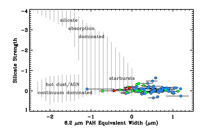
Figure 13: Equivalent width of the 6.2 µm PAH feature versus a silicate absorption strength, defined as the log of the ratio of the minimum in the 9.7 µm absorption trough to the interpolated value at this point from a linear fit to the 4.5–5 µm and 14.5–15 µm regions. SSGSS galaxies are colour-coded according to BPT designation (Kewley et al., 2001; Kauffmann et al., 2003b); blue points are star-forming galaxies, green points are composite sources, and red points are AGN. The shaded region shows the positions on this plot of LIRGs, ULIRGS, starbursts and AGN from Spoon et al. (2007). These more extreme galaxies tend to have stronger silicate absorption and brighter continua than the more quiescent star-forming galaxies of the SSGSS sample.

The shape of the MIR spectra of the most extreme IR emitters tends to be dominated by either a bright continuum — from either AGN or hot dust — or by heavy silicate absorption centered at $\sim 9.7$ µm. Spoon et al. (2007) (S07) showed that this gives rise to a bimodality in the space of 6.2 µm EW versus silicate absorption strength for ULIRGs and other IR-luminous galaxies and for AGN, from analysis of sources observed with Spitzer and ISO.

Figure 13 shows the location of the SSGSS galaxies in this space, with the regions occupied by the S07 sources shaded. We calculate our indicator of absorption strength similarly to the method used by S07 for starburst galaxies. We take the ratio of the 9.5–10.5 µm minimum to the “unabsorbed” flux at this point, the latter determined by interpolation using a linear fit between 4.5–5 µm and 14.5–15 µm regions, which are relatively unaffected by PAH emission or silicate absorption. 6.2 µm PAH EW is calculated using PAHFIT to measure the feature strength, as described in Treyer et al. (2010) (hereafter T10). This method differs from that used by S07, who determine the continuum, and hence the EW, by fitting a spline between the edges of the 6.2 µm feature.

Methods for EW determination based on estimation of the continuum from the boundaries of the 6.2 µm feature result in saturation at widths greater than $\sim$0.5–1 µm. This is due to the fact that, at higher line strengths, the continuum estimation includes increasing amounts of light from the 6.2 µm feature and the neighboring 7.7 µm PAH complex in the continuum estimation. At EW $\gtrsim 0.5$–1 µm the flux at the points typically used to estimate the continuum is in fact dominated by PAH emission. Sargsyan & Weedman (2009) report 6.2 µm EWs for SSGSS galaxies, finding $EW<1$ µm for the entire sample. They calculate EW using a continuum fit anchored at 5.5 µm and 6.9 µm. This approach, like the spline method, is vulnerable to underestimates and saturation at high EWs due to the presence of significant PAH flux in the regions used for continuum estimates. T10 presents an analysis of this effect, and a comparison with the Sargsyan & Weedman (2009) results. As many SSGSS galaxies have strong 6.2 µm features, it is important that their EWs be measured using full continuum+PAH profile fitting.

In Figure 13 we can see that SSGSS galaxies have silicate absorption indicators consistent with the low absorption locus. A number of our sources are consistent with the starburst galaxies in S07’s analysis, but much of our sample extends to significantly higher EWs, in part because of the EW saturation issue. Sources with AGN components by BPT designation (Baldwin et al., 1981; Kewley et al., 2001; Kauffmann et al., 2003b) have brighter continua, and hence lower EWs, than purely Star-Forming (SF) galaxies. These EWs may also have been reduce by destruction of PAH by the AGN.

7.3 PAH Contribution to the IR Luminosity

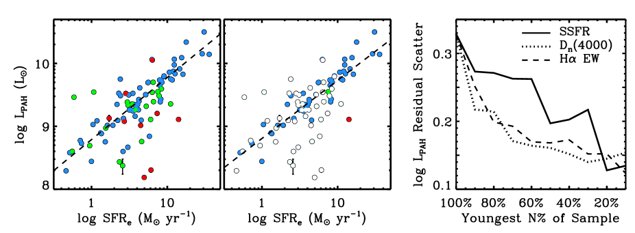
Figure 14: Left: total PAH luminosity versus SFR_e. Middle: as with the right panel, but, only galaxies with SSFR $<1\times 10^{-10}$ yr^-1 are filled, revealing an especially tight trend for galaxies dominated by young populations. Dashed lines show the best regression fits to star-forming galaxies (left) and the filled circles (middle). Right: standard deviation in the fractional residuals in infrared luminosity after subtraction of the best linear fit to the plot of $L_{PAH}$ $SFR_{e}$. For each point in this plot, the fit was made to the subset of the sample with specific star formation indicator (SSFR, $D_{n}(4000)$, or H$\alpha$ EW) below the given value. The trend indicates that, while young populations exhibit a very tight relationship between PAH or total IR luminosity and SFR, this relationship becomes increasingly scattered as populations age.

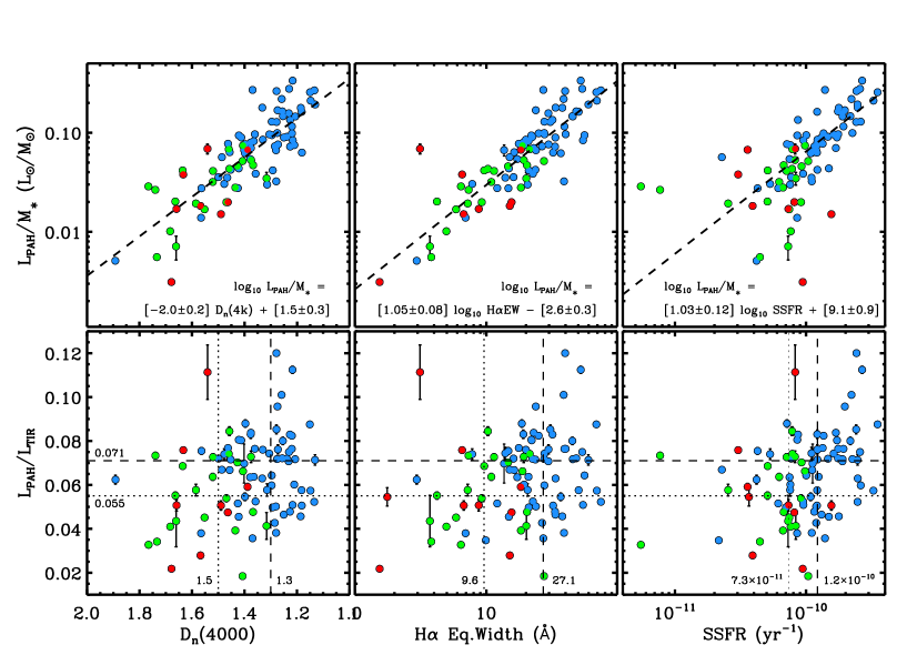
Figure 15: Upper: $L_{PAH}/M_{*}$ versus $D_{n}(4000)$ (left), H$\alpha$ EW (middle), and SSFR (right). Galaxies are colour-coded according to BPT type as in Figure 13. AGNs and composite sources sit on the same loci as SF galaxies, and have systematically older stellar populations. Dashed lines show regression fits for the SF population (blue points), with AGNs/composites excluded. Lower: As above, but for $L_{PAH}/L_{TIR}$. Dashed and dotted lines show the median values for SF galaxies and AGNs/composites respectively.

For star-forming galaxies, total infrared luminosity ($L_{TIR}$) is an good proxy for the rate of current star formation, with much of the starlight in dusty starburst environments being reprocessed into the IR. SSGSS has already shown that PAH emission is also strongly tied to a galaxy’s star formation history; the relative intensities of PAH bands trace specific star formation indicators (OD09), while the luminosities of individual PAH bands correlate strongly with total SFR (T10).

Understanding this latter relation, and in general the relative strength of the PAH contribution to galaxies’ MIR emission, is important for modeling the IR SEDs of higher redshift galaxies where the PAH bands cannot be so clearly resolved, and for SED modeling in large photometric surveys such as SWIRE (Lonsdale et al., 2003). T10 demonstrated the near-linearity of the relation between the intensity of individual PAH features and both $L_{TIR}$ and SFR. For the purpose of model fitting to MIR data in which individual PAH features are not well resolved, it is also valuable to determine the link between total PAH luminosity ($L_{PAH}$) and SFR and $L_{TIR}$.

We measure $L_{PAH}$ using PAHFIT (Smith et al. 2007; see Sect. 6.3), summing the integrated strengths of all PAH bands between, and including, the 6.2 µm to 17 µm features. The relatively weak 3.6 µm feature falls outside our spectral range and is not included in our determination of $L_{PAH}$. We correct $L_{PAH}$ for aperture effects, comparing SWIRE and SSGSS peak-up photometry to synthetic photometry (see Sect. 5.4), and interpolating corrections to PAH peak wavelengths. $L_{TIR}$ is determined by fitting Draine & Li (2007) model SEDs to the Spitzer (IRAC, IRS blue peak up, and MIPS) photometry, and then integrating between 3 and 1100 µm. SFR is from Brinchmann et al. (2004), who fit the models of Charlot & Longhetti (2001) to strong emission lines of galaxies in the SDSS spectroscopic sample, using a Kroupa IMF (Kroupa, 2001) and the Charlot & Fall (2000) dust model. We use the aperture-corrected median of the derived SFR likelihood distributions, designated $SFR_{e}$.

Figure 14 (left) shows $L_{PAH}$ versus $SFR_{e}$. These quantities are strongly correlated for the full SSGSS sample, however we are interested in calibrating $L_{PAH}$ to star formation, and so we perform regression analysis for SF galaxies only:

$$log_{10}~{}L_{PAH}(L_{\odot})=$$

$${}[0.99\pm 0.05]~{}log_{10}~{}SFR_{e}(M_{\odot}yr^{-1})+[8.8\pm 0.1]$$ (1)

The slope consistent with that presented in T10 for the 7.7 µm complex. As also found by T10, galaxies with AGN components generally fall on the same locus as purely star-forming galaxies, although have significantly greater scatter. This is primarily due to the fact that SFR is determined with much lower accuracy for the more evolved populations in which BPT-designated AGN are exclusively found.

This is further explored in Figure 14 (middle), which highlights the youngest 50% of the SSGSS sample, as defined by specific $SFR_{e}$ (SSFR; SSFR $>10^{-10}$ yr^-1), chosen simply to divide the sample in two. The correlation is significantly tighter when only these more actively star-forming galaxies are included. Fig. 14 (right) shows the standard deviation in the log residuals for $L_{PAH}$ after subtraction of the best linear fit for a range of subsample sizes. The subsamples are sorted to contain the youngest stellar populations, selected by three different measures: SSFR, $D_{n}(4000)$, and H$\alpha$ EW. In all cases, scatter decreases as the dominance of the young population increases; almost monotonically for $D_{n}(4000)$ and H$\alpha$ EW, and for these measures the scatter flattens significantly for the subsample containing the youngest $\sim$60% of sources, and for smaller “youngest” subsamples. The diagnostics corresponding to the $\sim 50^{th}$–$60^{th}$ percentile transition are $D_{n}(4000)=1.4$, H$\alpha$ EW $=18$Å, and SSFR $=10^{-10}$ yr^-1. For more evolved sources, the exceptionally tight trend between log $L_{PAH}$ and log $SFR_{e}$ ($\sigma<0.2$) gains significant scatter. Again, this is primarily due to the inaccuracy with which SFR is measured for evolved populations.

Figure 15 (upper panels) show the mass-weighted relationships. The ratio of $L_{PAH}$ to stellar mass ($M_{*}$ is plotted versus optical star formation diagnostics from SDSS: the narrow band 4000Å break measure $D_{n}(4000)$ (Kauffmann et al., 2003a) and H$\alpha$ EW (left and middle respectively), and also SSFR (right), which is described above. There are tight linear correlations between all quantities, although again we see the increased scatter in SFR for evolved galaxies. The best-fit regression lines for the SF galaxies are also shown. The mean 1-$\sigma$ residual scatter in $L_{PAH}/M_{*}$ for SF galaxies after subtraction of the best-fit lines is $\sim$20% for all three cases. For $D_{n}(4000)$ and H$\alpha$ EW, the residual is $\sim$20% even including galaxies with AGN components, indicating that these age diagnostics are good predictors of mass-weighted PAH intensity for most galaxies. This emphasizes that the increased scatter seen in $L_{PAH}$ and $L_{TIR}$ versus SFR in evolved populations is due to inaccuracy in measuring SFR rather than, say, a blurring due to evolved stars contributing more significantly to dust heating. As noted by Calzetti et al. (2010), the correlation between PAH emission and metallicity leads to another source of increased uncertainty in the link between star formation and IR dust emission in evolved sources.

Total IR luminosity is also closely related to these SF diagnostics, and has a very similar slope and scatter as $L_{PAH}$, for all three parameters and for both the absolute and mass-weighted relations. For the purpose of modeling high-z and photometric SEDS, it is useful to understand how the PAH-to-total IR ratio changes with these properties. Figure 15 (lower panels) show $L_{PAH}/L_{TIR}$ versus these same SF diagnostics, with dashed and dotted lines showing the medians for the SF and AGN/composite subsamples respectively. In all SF diagnostics there is a significant but highly scattered trend, with more evolved galaxies and AGN showing weaker PAH features for a given $L_{TIR}$. It is not possible to extricate the effects of age and AGN status on $L_{PAH}/L_{TIR}$ from these data, although as shown in OD09 both seem to play a part. More specifically, short wavelength PAH features (6.2 µm and 7.7 µm) are diminished in more evolved galaxies and AGN, while longer wavelength features are not. This is seen in the PAH ratios (OD09) and with respect to $L_{TIR}$ (T10). The trend is between $L_{PAH}/L_{TIR}$ and star formation is still weakly significant for SF galaxies alone, with AGN excluded, although this is entirely driven by a small number of heavily star-forming sources with very high $L_{PAH}/L_{TIR}$.

7.4 Dust Mass

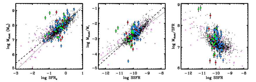
Figure 16: Left: dust masses for SSGSS galaxies from models of Draine & Li (2007) versus SFR_e (Brinchmann et al., 2004) (coloured circles, coded by BPT designation; see Fig. 13). Also plotted are the results of the dust model of da Cunha et al. (2010) for SDSS galaxies (black points) and SINGS galaxies (pink crosses). The best log-log regression lines are shown for SSGSS (dashed) and SDSS (dotted). Middle: dust-to-stellar mass fraction versus SSFR, and right: dust mass-to-SFR ratio.

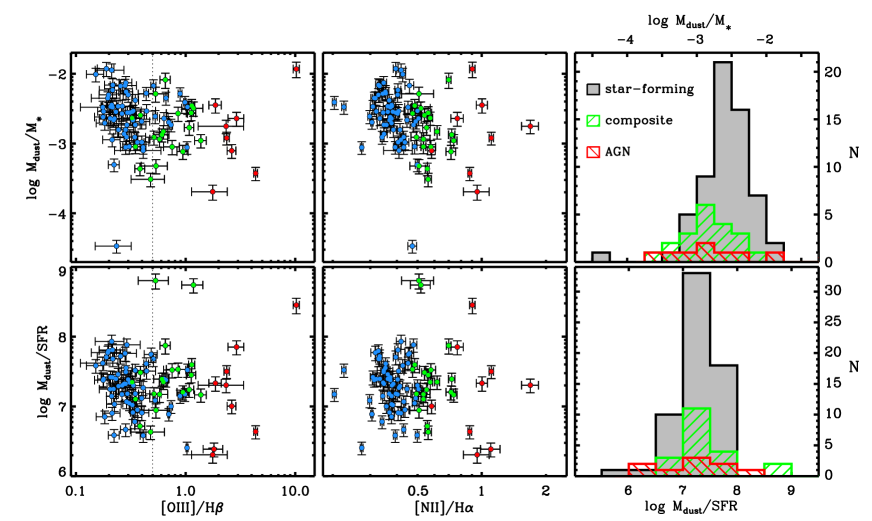
Figure 17: Upper Panels: dust-to-stellar mass fraction versus the optical emission line ratios [OIII]/H$\beta$ (left) and [NII]/H$\alpha$ (middle). These line ratios define BPT AGN type, which is designated by the same colour coding as Fig. 13. Also shown is the distribution of dust fractions by AGN type (right). AGN have significantly lower dust fractions than SF galaxies. SF galaxies with [OIII]/H$\beta>0.5$ (dotted line) are young galaxies with starburst-source hard radiation fields; these galaxies have significantly higher dust fractions than AGN with similar [OIII]/H$\beta$. Lower Panels: same as above, except with the ratio of dust mass to SFR_e.

The SSGSS IR spectra, with its coverage of all major PAH features, combined with MIPS 70 µm and 160 µm photometry, enables us to fit detailed dust models to determine dust mass. We use the models of Draine & Li (2007), which calculate IR emission spectra for starlight-heated dust consisting of amorphous silicate and graphite grains, and of PAH grains. SSGSS spectra and photometry are fit to template libraries derived from these models (Draine & Li, private communication) to estimate the distribution of illuminating starlight intensity and the relative abundance of PAH. These are combined with MIPS fluxes and the relations detailed in Draine & Li (2007) to determine the total dust mass.

Based on these models, the median dust mass for the sample is $M_{dust}=8.5\times 10^{7}$ M_⊙, with 90% of the sample in the range $10^{7}$—$10^{9}$ M_⊙.

Figure 16 (left) shows the calculated dust masses for the SSGSS sample versus SFR_e, with colour coding to indicate AGN type by BPT designation. Also plotted are the results of da Cunha et al. (2010) (D10), who fit the GALEX-SDSS-2MASS-IRAS photometry of SDSS and SINGS galaxies with SEDs derived from population synthesis and dust attenuation models (da Cunha, Charlot & Elbaz, 2008) to calculate both dust mass and SFR. SSGSS dust masses are very similar to the D10 SDSS sample. The SINGS dust masses are roughly consistent with the range of dust masses calculated using the Draine & Li (2007) models for a sub-sample of SINGS galaxies (Draine et al. (2007)), which reinforces the comparibility of the two models.

M_dust is highly correlated with SFR_e, with an almost linear relationship that is similar to that found by D10. The best-fit regression line is:

$$M_{dust}(M_{\odot})=$$

$${}(2.0\pm 0.3)\times 10^{7}~{}SFR_{e}(M_{\odot}yr^{-1})^{(0.95\pm 0.11)}$$ (2)

We note that D10 find a tighter relation between these two parameters for SDSS galaxies. This may indicate a more accurate SFR estimation by D10 over the optical emission line estimate, due to their use of the full FUV-to-FIR SED.

Figure 16 (middle) shows dust-to-stellar mass fraction versus SSFR for SSGSS, again including the results of D10. There is a significant positive correlation between dust fraction and SSFR ($\tau=0.24$; correlation significance: $p=0.001$), although here there is significantly more scatter than observed by D10 in their sample. The best-fit regression line is:

$$M_{dust}/M_{\odot}=(2.5\pm 1.0)\times 10^{5}~{}SSFR(yr^{-1})^{(0.8\pm 0.2)}$$ (3)

Figure 16 (right) shows the ratio of dust mass to SFR, which, given the tight correlation between SFR and gas mass, may be considered a proxy for the dust-to-gas mass ratio, and so traces the enrichment of the interstellar medium. The SSGSS results follow the general trend of the D10 sample, ($\tau=-0.175$; correlation significance: $p=0.015$), however the careful sample selection of SSGSS means that it contains fewer of the rare, extreme SF galaxies, and the UV selection eliminates the oldest red, dead galaxies; the result is a more restricted range of SSFR that makes it difficult to verify the slope of this relation.

These strong correlations between galaxys’ dust content and star formation rate — and especially between their absolute values — supports the idea that SFR provides a useful proxy for dust mass, as found by D10. The careful sample selection of SSGSS adds weight to this result.

As noted by D10, these relations can be interpreted in evolutionary terms. The ISM is enriched by dust with ongoing star formation, and at the same time gas mass decreases, resulting in a drop in SFR. With this drop, the production of dust is quickly superseded by destruction of grains in the ISM, resulting in the positive correlation between dust fraction and SSFR (Fig. 16, middle). At the same time, this reduction in dust content with galaxy age appears to be outpaced by the reduction in gas content and the associated drop in SSFR, resulting in the anticorrelation between dust-to-gas mass ratio vs. SSFR (Fig. 16, right).

In this scenario, the balance between ISM enrichment and the destruction of dust by shocks and by the ambient radiation field defines the direction and slope of these relations. The BPT emission line ratios, [OIII]/H$\beta$ and [NII]/H$\alpha$, are sensitive to the hardness of the ambient radiation field and the level of ISM enrichment respectively, and so may shed light on the nature of this balance. Additionally, as seen in Figure 16, galaxies with BPT-designated AGN components have lower dust fractions than SF galaxies. Although this may be purely due to the increased incidence (and observability) of AGN in older galaxies, the difference in dust fraction with SSFR seems to be divided surprisingly cleanly down AGN lines. It is possible that AGN shocks and hard UV photons are important in destroying small dust grains, given their potential affect on PAH grain size distributions (Smith et al. 2007; OD09; T10)

Figure 17 (upper panels) shows dust-to-stellar mass fraction versus [OIII]/H$\beta$ and [NII]/H$\alpha$, as well as the distribution of dust fractions by BPT designation. Both ratios show a scattered but significant inverse correlation, and in both cases there is no significant trend taking either SF galaxies or AGN separately.

[OIII]/H$\beta$ provides a good proxy for the hardness of the UV radiation field, and so it is tempting to link dust grain destruction with an increase in hard UV photons, although it is not possible to extricate this effect from the drop in dust production with diminishing star formation. Notably, SF galaxies with hard UV fields ([OIII]/H$\beta\gtrsim$ 0.5) all have have significantly higher dust fractions than AGN with similar [OIII]/H$\beta$. These same galaxies have among the highest SSFRs, implying that either the radiation field has little to do with grain destruction, or that dust production due to heavy star formation in these galaxies more than compensates for such depletion.

[NII]/H$\alpha$ is sensitive to gas-phase metallicity, and so may be expected to have a positive correlation with dust-to-stellar mass fraction. The observed negative correlation supports the idea that the drop in dust content of these galaxies ($M_{dust}/M_{*}$) outpaces the increase in the gas-phase metallicity (and corresponding dust-to-gas mass fraction) as these galaxies evolve.

Figure 17 (lower panels) shows the ratio of dust mass to SFR vs. BPT line ratios. There is no correlation between this and any of the line ratios, and no trend with AGN status. This is expected; while dust-to-stellar mass fraction decreases with stellar population age, gas content and the associated SFR probably decreases more quickly, eliminating any trend.

Dust masses for the entire SSGSS sample are available as part of the data release (see Sect. 8.2)

8 Data Products and Value-Added Catalogs

8.1 Spitzer Data Archive

SSGSS is a Spitzer Legacy Program, and all spectroscopy is available for download from the Spitzer Data Archive. The archive is accessed via Spitzer’s Leopard software. The web interface for the archive and link to the Leopard download page can be found at: http://archive.spitzer.caltech.edu/.

The data release includes low-resolution spectra of the 100 galaxies in the full SSGSS sample and high-resolution spectra of the 33 galaxies in the bright SSGSS sample. These are reduced as described in Section 5. We include spectra with slit positions both combined and uncombined, and with orders and (for low-res) SL and LL modules both stitched and unstitched.

8.2 Complementary Data Products

In addition to the spectroscopic data, a range of complementary data products are available via the SSGSS website:

http://astro.columbia.edu/ssgss

UV through IR imaging data: including FUV and NUV from GALEX; ugriz from SDSS; IRAC 3.6, 4.5, 5.8, and 7.8 µm bands; MIPS 24, 70, and 160 µm bands; and 16 µm IRS Peakup from SSGSS, with corresponding uncertainty and/or background images.

Matched catalogs of SDSS properties: these are from the SDSS studies at MPA/JHU group (Brinchmann et al., 2004), and are drawn from data release 4 of their catalogs. These include measured and derived parameters such as magnitudes, line strengths, Petrosian radii, SFRs, and index strengths, as well as magnitudes K-corrected using the method of Blanton et al. (2006), stellar masses, mass-to-light ratios, dust attenuations, etc. from Kauffmann et al. (2003a), and gas-phase metallicities from Tremonti et al. (2004).

PAH strengths: integrated intensities for the most prominent PAH features and complexes at 6.2 µm, 7.7 µm, 8.6 µm, 11.3 µm, and 17 µm, as well as total PAH intensity, measured by the PAHFIT (Smith et al., 2007) decompositions of SSGSS spectra as described in OD09.

Emission line strengths: line strengths from both the low-res and hi-res spectra from PAHFIT decompositions.

Derived properties: dust masses (see Sect. 7.4), silicate strength (see Sect. 7.2), and silicate optical depth from PAHFIT decompositions.

9 Summary

We have presented SSGSS, a new Spitzer spectroscopic survey of galaxies, colour-selected to be representative of the normal, star-forming galaxy population. SSGSS targets 101 galaxies in the Lockman Hole, all with extensive ancilliary imaging and spectroscopy from the FUV to the FIR. All galaxies were observed with IRS low resolution modules from 5—40 µm and a subsample of the 33 brightest were observed with at high resolution from 10—20 µm.

For the low resolution spectra, our target S/N of 5 per resolution element was exceeded except in some SL2 spectra and in regions of high silicate absorption around 10µm. At high resolution, S/N $>$ 10 was achieved for all but one [Ne II] lines and S/N $>$ 10 for $\sim$90% of [Ne III] lines. Of the 101 observed galaxies, 100 resulted in useful spectra, which are available from the Spitzer archive.

Comparison of SSGSS galaxies to starbursts shows that the starburst spectra differ primarily in the shape of the warm dust continuum, consistent with having elevated emission at small-grain dust temperatures of $\lesssim 120$ K. Silicate absorption levels of SSGSS galaxies are uniformly lower than those often observed in LIRGs and ULIRGs, and are similar to those observed in starbursts.

Using PAH strengths measured with the PAHFIT code of Smith et al. (2007), we have investigated the link between total PAH emission and both IR luminosity and star formation indicators. PAH luminosity correlates with star formation indicators $D_{n}(4000)$ and H$\alpha$ EW very tightly, except for the oldest $\sim$20% of the sample. PAH-to-total IR luminosity ratio changes slightly between SF galaxies and those with AGN components, dropping from $\sim$0.07 to $\sim$0.05. This approximately reflects the change between actively star forming galaxies and more evolved galaxies.

Dust masses calculated from the models of Draine & Li (2007) reveal a close relationship between dust mass and SFR, and are consistent with the evolutionary scenario described by D10 in which dust that is produced quickly in a rapidly star-forming phase is destroyed more quickly than it is replenished as star formation drops.

SSGSS offer great scope for further study. In OD09, the sample has been used to conduct a detailed analysis of the physical drivers of PAH spectral shapes, and Treyer et al. (2010) investigates the use of MIR diagnostics for SF and AGN activity. Future work will include the development of template PAH spectra calibrated to a wide range of observables, analysis of the role of the size, shape, and composition (via metallicity) of small dust grains in determining the continuum shape.

Appendix A: Multi-Wavelength Thumbnails

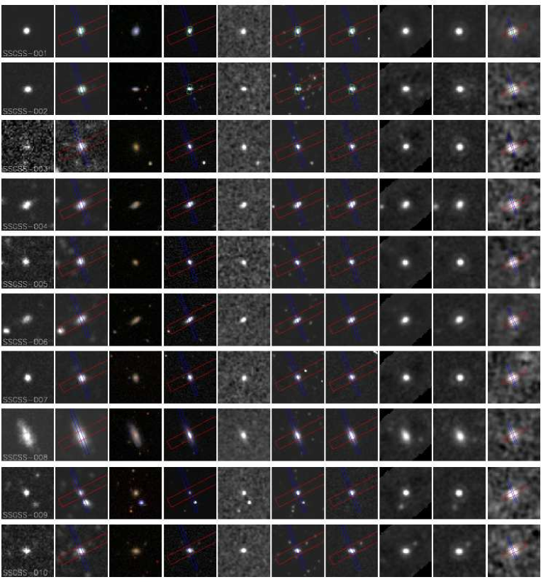
FUV     NUV     SDSS        r          H       3.6 µm    8 µm     16 µm    25 µm   70 µm

Figure 18: Multi-wavelength images of the 101 galaxies of the SSGSS sample. Each horizontal strip shows a given galaxy in, respectively: GALEX FUV and NUV, SDSS multi-colour, r, H, IRAC 3.6 µm and 8 µm, 16 µm from SSGSS peakup images, and MIPS 25 µm and 70 µm. All boxes are 60″ on a side except for the 70 µm band, which is 120″.

FUV     NUV     SDSS        r          H       3.6 µm    8 µm     16 µm    25 µm   70 µm
Figure 18 (continued)

FUV     NUV     SDSS        r          H       3.6 µm    8 µm     16 µm    25 µm   70 µm
Figure 18 (continued)

FUV     NUV     SDSS        r          H       3.6 µm    8 µm     16 µm    25 µm   70 µm
Figure 18 (continued)

FUV     NUV     SDSS        r          H       3.6 µm    8 µm     16 µm    25 µm   70 µm
Figure 18 (continued)

FUV     NUV     SDSS        r          H       3.6 µm    8 µm     16 µm    25 µm   70 µm
Figure 18 (continued)

FUV     NUV     SDSS        r          H       3.6 µm    8 µm     16 µm    25 µm   70 µm
Figure 18 (continued)

FUV     NUV     SDSS        r          H       3.6 µm    8 µm     16 µm    25 µm   70 µm
Figure 18 (continued)

FUV     NUV     SDSS        r          H       3.6 µm    8 µm     16 µm    25 µm   70 µm
Figure 18 (continued)

FUV     NUV     SDSS        r          H       3.6 µm    8 µm     16 µm    25 µm   70 µm
Figure 18 (continued)

Appendix B: Reduced IRS Spectra

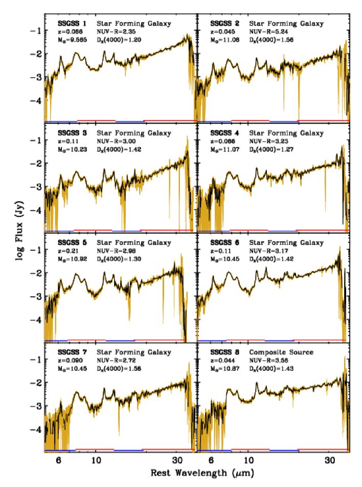
Figure 19: Short-low and long-low IRS spectra, reduced and stitched as described in Section 5.1. The yellow shaded region shows the $\pm 1$-sigma errors. The wavelength range of each IRS module is shown at the base of each panel, from left to right: SL2 (blue), SL1 (red), LL2 (blue), LL1 (red). Also given are the SSGSS catalog number, BPT type (Baldwin et al., 1981), redshift, stellar mass, NUV-R color, and $D_{n}(4000)$ age diagnostic.

Figure 19 (continued)

Figure 19 (continued)

Figure 19 (continued)

Figure 19 (continued)

Figure 19 (continued)

Figure 19 (continued)

Figure 19 (continued)

Figure 19 (continued)

Figure 19 (continued)

Figure 19 (continued)

Figure 19 (continued)

Figure 19 (continued)

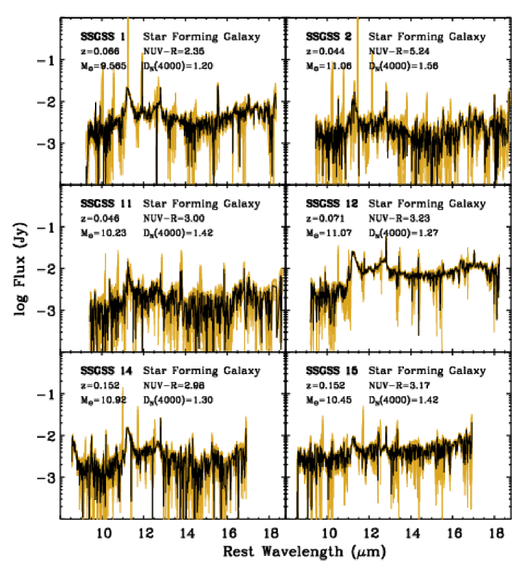
Figure 20: Short-high IRS spectra, reduced and stitched as described in Section 5.2. The yellow shaded region shows the $\pm 1$-sigma errors. Also given are the SSGSS catalog number, BPT type (Baldwin et al., 1981), redshift, stellar mass, NUV-R color, and $D_{n}(4000)$ age diagnostic.

Figure 20 (continued)

Figure 20 (continued)

Figure 20 (continued)

Figure 20 (continued)

Figure 20 (continued)

References

- Baldwin et al. (1981) Baldwin J., Phillips M., & Terlevich R., 1981, PASP, 93, 5
- Balogh et al. (2004) Balogh, M. L., Baldry, I. K., Nichol, R., Miller, C., Bower, R., Glazebrook, K., 2004, ApJL, 615, L101
- Beichman et al. (2003) Beichman, C. A., Cutri, R., Jarrett, T., Stiening, R., Skrutskie, M., 2003, AJ, 125, 2521
- Bell & Kennicutt (2001) Bell, E. F., Kennicutt, R. C. 2001, ApJ, 548, 681
- Bell et al. (2003) Bell, E. F., McIntosh, D. H., Katz, N., Weinberg, M. D., 2003, ApJS, 149, 289
- Bell et al. (2005) Bell, E. F., Papovich, C., Wolf, C., et al., 2005, ApJ, 625, 23
- Bernard-Salas et al. (2009) Bernard-Salas, J., Spoon, H. W. W., Charmandaris, V., et al., 2009, ApJS, 184, 230
- Blanton et al. (2003a) Blanton, M. R., Hogg, D. W., Bahcall, N. A., et al., 2003, ApJ, 594, 186
- Blanton et al. (2003b) Blanton, M. R., Lin, H., Lupton, R., H., Miller Maley, F., Young, N., Zehavi, I., Loveday, J., 2003, AJ, 125, 2276
- Blanton et al. (2006) Blanton, M. R., Eisenstein, D., Hogg, D. W., Zehavi, I., 2006, ApJ, 645, 977
- Brandl et al. (2006) Brandl, B. R., Bernard-Salas, J., Spoon, H. W. W., et al., 2006, ApJ, 653, 1129
- Brinchmann et al. (2004) Brinchmann, J., Charlot, S., White, S. D. M., Tremonti, C., Kauffmann, G., Heckman, T., Brinkmann, J., 2004, MNRAS, 351, 1151
- Buat & Xu (1996) Buat, V. & Xu, C., 1996, A&A, 306, 61()]
- Buat, Bavazzi & Bonfanti (02) Buat, V., Boselli, A., Gavazzi, G., Bonfanti, C., 2002, A&A, 383, 801
- Calzetti, Kinney, & Storchi-Bergmann (1994) Calzetti, D., Kinney, A. L., & Storchi-Bergmann, T., 1994, ApJ, 429, 582
- Calzetti (2001) Calzetti, D., 2001, PASP, 113, 1449
- Calzetti et al. (2010) Calzetti, D., Wu, S.-Y., Hong, S., et al., 2010, ApJ, 714, 1256
- Charlot & Fall (2000) Charlot, S., Fall, S. M. 2000, ApJ, 539, 718
- Charlot & Longhetti (2001) Charlot, S., Longhetti, M., 2001, MNRAS, 323, 887
- da Cunha, Charlot & Elbaz (2008) da Cunha, E., Charlot, S., Elbaz, D., 2008, MNRAS, 388, 1595
- da Cunha et al. (2010) da Cunha, E., Eminian, C., Charlot, S., Blaizot, J., 2010, MNRAS, 403, 1894
- Dale et al. (2009) Dale, D. A., Smith, J. D. T., Schlawin, E. A., et al., 2009, ApJ, 693, 1821
- Dasyra et al. (2009) Dasyra, K. M., Yan, L., Helou, G., et al., 2009, ApJ, 701, 1123
- Desai et al. (2009) Desai, V., Soifer, B. T., Dey, A., et al., 2009, ApJ, 700, 1190
- Devereux & Young (1991) Devereux, N. A. & Young, J. S., 1991, ApJ, 371, 515
- Draine & Li (2001) Draine, B. T., Li, A. 2001, ApJ, 551, 807
- Draine & Li (2007) Draine, B. T. & Li, A., 2007, ApJ, 551, 807
- Draine & Li (2007) Draine, B. T. & Li, A., 2007, ApJ, 657, 810
- Draine et al. (2007) Draine, B. T., Dale, D. A., Bendo, G., et al., 2007, ApJ, 663,866
- Galliano et al. (2008) Galliano, F., Madden, S. C., Tielens, A. G. G. M., Peeters, E., & Jones, A. P. 2008 ApJ, 679, 310
- Goldader et al. (2002) Goldader, J. D., Meurer, G., Heckman, T. M., Seibert, M., Sanders, D. B., Calzetti, D., Steidel, C. C., 2002, ApJ, 568, 651
- Hanish et al. (2010) Hanish, D. J., Oey, M. S., Rigby, J. R., de Mello, D. F., Lee, J. C., 2010, ApJ,
- Heckman et al. (2005) Heckman, T. M., Hoopes, C. G., Seibert, M., et al., 2005, ApJL, 619, L35
- Helou (1986) Helou, G., 1986, ApJ, 311, L33
- Helou et al. (2000) Helou, G., Lu, N. Y., Werner, M. W., Malhotra, S., & Silbermann, N., 2000, ApJ, 352, L21
- Hernán-Caballero et al. (2009) Hernán-Caballero, A., Pérez-Fournon, I., Hatziminaoglou, E., et al., 2009, MNRAS, 395, 1695
- Imanishi, Maiolino & Nakagawa (2010) Imanishi, M., Maiolino, R., & Nakagawa, T., 2010, ApJ, 709, 801
- Johnson et al. (2006) Johnson, B. D., Schiminovich, D., Seibert, M., et al., 2006, ApJL, 644, L109
- Johnson et al. (2007) Johnson, B. D., Schiminovich, D., Seibert, M., et al., 2007, ApJS, 173, 392
- Kauffmann et al. (2004) Kauffmann, G., White, S. D. M., Heckman, T. M., Ménard, B., Brinchmann, J., Charlot, S., Tremonti, C., Brinkmann, J., 2004, MNRAS, 353, 713
- Kauffmann et al. (2003a) Kauffmann, G., Heckman, T., White, S. D. M., et al., 2003, MNRAS, 341, 33
- Kauffmann et al. (2003b) Kauffmann G., Heckman T., Tremonte C., et al., 2003, MNRAS, 346, 1055
- Kennicutt (1998) Kennicutt, R. C., 1998, ApJ, 498, 541
- Kennicutt et al. (2003) Kennicutt, R. C., Jr., Armus, L., Bendo, G., et al. 2003, PASP, 115, 928
- Kewley et al. (2001) Kewley L., Dopita M., Sutherland R., Heisler C. & Trevena J., 2001, ApJ, 556, 121
- Kewley et al. (2002) Kewley, L. J., Geller, M. J., Jansen, R. A., & Dopita, M. A., 2002, AJ, 124, 3135
- Kroupa (2001) Kroupa, P. 2001, MNRAS, 322, 231
- Le Floc’h et al. (2005) Le Floc’h, E., Papovich, C., Dole, H, et al., 2005, ApJ, 632, 169
- Lonsdale et al. (2003) Lonsdale, C. J., Smith, H. E., Rowan-Robinson, M., et al., 2003, PASP, 115, 897
- Malhotra et al. (2001) Malhotra, S., et al., 2001, ApJ, 561, 766
- Martin et al. (2005) Martin, C. D., Fanson, J., Schiminovich, D., et al., 2005, ApJ, 619, L1
- Melbourne, Koo & Le Floc’h (2005) Melbourne, J., Koo, D. C., Le Floc’h, E., 2005, ApJL, 632, L65
- Moustakas et al. (2010) Moustakas, J, Kennicutt, R. C., Jr., Tremonti, C. A., Dale, D. A., Smith, J. D. T., Calzetti, D., 2010, ApJS, 190, 233
- Muñoz-Mateos et al. (2009a) Muñoz-Mateos, J. C., Gil de Paz, A., Zamorano, J., et al., 2009, ApJ, 703, 1569
- Muñoz-Mateos et al. (2009b) Muñoz-Mateos, J. C., Gil de Paz, A., Boissier, S., et al., 2009, ApJ, 701, 1965
- Muñoz-Mateos et al. (2011) Muñoz-Mateos, J. C., Boissier, S., Gil de Paz, A., et al., 2011, ApJ, (accepted; arXiv/1102.1724)
- Murphy et al. (2009) Murphy, E. J., Chary, R.-R., Alexander, D. M., Dickinson, M., Magnelli, B., Morrison, G., Pope, A., Teplitz, H. I., 2009, ApJ, 698, 1380
- Noeske et al. (2007) Noeske, K. G., Faber, S. M., Weiner, B. J., et al., 2007, ApJL, 660, L43
- O’Dowd et al. (2009) O’Dowd, M., Schiminovich, D., Johnson, B., et al 2009, ApJ, 705, 885
- Perez-Gonzalez et al. (2005) Perez-Gonzalez, P. G., , Rieke, G. H., Egami, E., et al., 2005, ApJ, 630, 82
- Peeters, Spoon & Tielens (2004) Peeters, E., Spoon, H. W. W., Tielens, A. G. G. M., 2004, ApJ, 613, 986
- Prescott et al. (2007) Prescott, M. K. M., Kennicutt, R. C., Jr., Bendo, G. J., et al., 2007, ApJ, 668, 182
- Roussel et al. (2007) Roussel, H., Helou, G., Hollenbach, D. J., et al., 2007, ApJ, 669, 959
- Rowan-Robinson & Crawford (1989) Rowan-Robinson, M. & Crawford, J., 1989, MNRAS, 238, 523
- Sargsyan & Weedman (2009) Sargsyan, L. A., Weedman, D. W., 2009, ApJ, 701, 1398
- Sauvage & Thuan (1992) Sauvage, M. & Thuan, T. X., 1992, ApJ, 396, L69
- Schutte et al. (1993) Schutte, W. A., Tielens, A. G. G. M., & Allamandola, L. J., 1993, ApJ, 415, 397
- Smith (2004) Smith, J. D. T., 2004, Calibrating Extended Sources with the IRS
- Smith et al. (2007) Smith J. D. T., Draine B. T., Dale D. A., et al. 2007, ApJ, 656, 770
- Sullivan (2000) Sullivan, M., Treyer, M. A., Ellis, R. S., Bridges, T. J., Milliard, B., Donas, J. 2000, MNRAS, 312, 442
- Spoon et al. (2002) Spoon, H. W. W., Keane, J. V., Tielens, A. G. G. M., Lutz, D., Moorwood, A. F. M., Laurent, O, 2002, A&A, 385, 1022
- Spoon et al. (2007) Spoon, H. W. W., Marshall, A., Houck, J. R., et al., 2007, ApJ, 654, L49
- Sturm et al (2000) Sturm, E., Lutz, D., Tran, D., et al., 2000, A&A, 358, 481
- Teplitz et al. (2007) Teplitz, H. I.,Desai, V., Armus, L., et al., 2007, ApJ, 659, 941
- Tielens (2005) Tielens, A. G. G. M. 2005, The Physics and Chemistry of the Interstellar Medium, Cambridge University Press
- Tremonti et al. (2004) Tremonti, C, A., Heckman, T. M., Kauffmann, G., et al., 2004, ApJ, 613, 898
- Treyer et al. (2010) Treyer, M., Schminovich, D., Johnson, B., O’Dowd, M., et al., 2010, ApJ, 719, 1191
- Walterbos & Greenawalt (1996) Walterbos, R. A. M. & Greenawalt, B., 1996, ApJ, 460, 696
- Wang & Heckman (1996) Wang, B., Heckman, T. M. 1996, ApJ, 457, 645
- Weedman et al. (2006) Weedman, D., Polletta, M., Lonsdale, C. J., Wilkes, B. J., Siana, B., Houck, J. R., Surace, J., Shupe, D., Farrah, D., Smith, H. E., 2006, ApJ, 653, 101
- Yan et al. (2005) Yan, L., Dickinson, M., Stern, D., et al., 2005, ApJ, 628, 604
- Yan et al. (2007) Yan, H., Dickinson, M., Giavalisco, M., Stern, D., Eisenhardt, P. R. M., Ferguson, H. C., 2007, in Astronomical Society of the Pacific Conference Series, Vol. 380, Astronomical Society of the Pacific Conference Series, ed. J. Afonso, H. C. Ferguson, B. Mobasher, & R. Norris, 35 Yan, L., Dickinson, M., Stern, D., et al., 2005, ApJ, 628, 604
- Yi et al. (2005) Yi, S. Y., Yoon, S.-J., Kaviraj, S., et al., 2005, ApJL, 619, L111
- York et al. (2000) York, D.G., Adelman, J., Anderson, J.E., et al. 2000, AJ, 120, 1579
- Zheng et al. (2007) Zheng, X. Z., Xian Z., Dole, H., Bell, E. F., Le Floc’h, E., Rieke, G. H., Rix, H.-W., Schiminovich, D., 2007, ApJ, 670, 301