Evidence of Critical Balance in Kinetic Alfvén Wave Turbulence Simulations

Abstract

A numerical simulation of kinetic plasma turbulence is performed to assess the applicability of critical balance to kinetic, dissipation scale turbulence. The analysis is performed in the frequency domain to obviate complications inherent in performing a local analysis of turbulence. A theoretical model of dissipation scale critical balance is constructed and compared to simulation results, and excellent agreement is found. This result constitutes the first evidence of critical balance in a kinetic turbulence simulation and provides evidence of an anisotropic turbulence cascade extending into the dissipation range. We also perform an Eulerian frequency analysis of the simulation data and compare it to the results of a previous study of magnetohydrodynamic turbulence simulations.

I Introduction

Plasma turbulence is ubiquitous in a wide range of space and astrophysical environments, playing a fundamental role in transferring energy from the large scales at which the turbulence is driven to the small scales at which the turbulence is dissipated. Developing a detailed understanding of plasma turbulence is one of the key goals of the space physics and astrophysics communities.

One of the central tenets of plasma turbulence is the concept of critical balance. Critical balance is the supposition that the time scale associated with linear fluctuations of Alfvén waves, $\omega=k_{\parallel}v_{A}$, is of the same order of magnitude as time scale associated with the nonlinear cascade of energy, $\omega_{nl}\simeq k_{\perp}v_{\perp}$, where $v_{A}$ is the Alfvén speed, $v_{\perp}$ is the perpendicular fluctuation velocity, and parallel and perpendicular are defined with respect to the direction of the local mean magnetic field Goldreich and Sridhar (1995, 1997); Maron and Goldreich (2001). Critical balance leads to the prediction of an anisotropic cascade of energy in wavevector space, where magnetic energy cascades at different rates parallel and perpendicular to the local mean magnetic field.

Although the original predictions of critical balance pertain only to a cascade of Alfvén waves in the magnetohydrodynamic (MHD) limit of the inertial range, the theory can be extended to scales smaller than the ion gyroradius, at which wave-particle damping and collisions become important Cho and Lazarian (2004); Galtier (2006); Howes et al. (2008); Schekochihin et al. (2009). The latter region is often referred to as the dissipation range of plasma turbulence, where it is proposed that the cascade of Alfvén waves transitions to a cascade of kinetic Alfvén waves (KAW) Howes et al. (2008, 2008); Schekochihin et al. (2009).

The anisotropic scaling of the magnetic field energy has been observed in the inertial range portion of the solar wind through the use of wavelets or second-order structure functions to discern the local mean magnetic field direction, e.g., Horbury et al. (2008); Podesta (2009); Chen et al. (2010); Wicks et al. (2010); Luo and Wu (2010). Horbury et al. (2008) demonstrated that critical balance fits the solar wind observations well in the directions parallel and perpendicular to the local mean magnetic field, and Forman et al. (2011) went further, demonstrating that solar wind observations follow the predictions of critical balance for all angles between parallel and perpendicular.

Critical balance and its physical consequences have also been tested and verified in many numerical turbulence simulations. It has been tested extensively in MHD simulations, e.g., Cho and Vishniac (2000); Maron and Goldreich (2001); Cho et al. (2002); Cho and Lazarian (2003); Oughton et al. (2004), and at smaller, dissipation range scales in electron MHD (EMHD) simulations, e.g., Cho and Lazarian (2004, 2009). However, all of the previous studies have been performed with fluid codes that cannot capture wave-particle interactions nor accurately model collisional effects, both of which play important roles in dissipating turbulence at scales below the ion gyroradius.

To evaluate whether critical balance persists in the dissipation range, we consider here a detailed study of a numerical simulation of dissipation scale turbulence performed using AstroGK, the Astrophysical Gyrokinetics Code, developed to study kinetic turbulence in astrophysical environments. Rather than examining the energy distribution in wavenumber space, we perform our analysis in the frequency domain to obviate some of the difficulties inherent in performing a local analysis of turbulence, which are discussed in §VI. The frequency is used as a proxy for the parallel wavenumber to determine whether or not an anisotropic cascade, consistent with that predicted for critically balanced kinetic Alfvén wave turbulence, exists in the dissipation range. An Eulerian frequency analysis of the AstroGK simulation will also be compared to a similar study by Dmitruk and Matthaeus (2009) performed using a MHD simulation.

II Simulation Parameters

A detailed description of AstroGK and the results of linear and nonlinear benchmarks are presented in Numata et al. (2010), so we provide here only a brief overview.

AstroGK is an Eulerian slab code with triply periodic boundary conditions that solves the electromagnetic gyroaveraged Vlasov-Maxwell five dimensional system of equations. It solves the gyrokinetic equation and gyroaveraged Maxwell’s equations for the perturbed gyroaveraged distribution function, $h_{s}(x,y,z,\lambda,\epsilon)$, for each species $s$ (protons and electrons), the parallel vector potential, $A_{z}$, and perturbed parallel magnetic field, $\delta B_{z}$, and the scalar potential, $\phi$ Frieman and Chen (1982); Howes et al. (2006). The simulation domain is elongated along the direction of the equilibrium magnetic field $\mathbf{B}_{0}=B_{0}\hat{\bz}$. Velocity space coordinates are related to the energy, $\epsilon=v^{2}/2$, and pitch angle, $\lambda=v_{\perp}^{2}/v^{2}$. The equilibrium distribution for both species is treated as Maxwellian, and a realistic mass ratio, $m_{p}/m_{e}=1836$, is used. The $x-y$ plane is treated pseduospectrally, and an upwinded finite-differencing approach is employed for the $z$-direction. Velocity space is evaluated following Gaussian quadrature rules. Linear terms are evolved implicitly in time, while nonlinear terms are evolved explicitly by a third-order Adams-Bashforth method. Collisions are treated using a fully conservative, linearized, and gyroaveraged collision operator Abel et al. (2008); Barnes et al. (2009).

To represent average solar wind conditions observed at $\simeq 1$ AU, we choose plasma parameters $\beta_{i}=1$ and $T_{i}=T_{e}$, where $\beta_{i}=v_{ti}^{2}/v_{A}^{2}$, $v_{A}=B_{0}/\sqrt{4\pi n_{0i}m_{i}}$, and $v_{ti}=\sqrt{2T_{i}/m_{i}}$ is the ion thermal speed. We output the electromagnetic field information at fixed time intervals. Since this diagnostic is data intensive, we choose to perform the simulation on a numerical grid smaller than the largest simulations performed with AstroGK Howes et al. (2011). Specifically, we use a numerical grid of $(n_{x},n_{y},n_{z},n_{\epsilon},n_{\lambda},n_{s})=$ $(32,32,64,16,16,2)$, where $n_{\epsilon}$, $n_{\lambda}$, and $n_{s}$ are the number of grid points in energy, pitch angle, and species respectively. The spatial extent of the domain is $(L_{x},L_{y},L_{z})=2\pi(\rho_{i},\rho_{i},a_{0})$, where $\rho_{i}=v_{ti}/\Omega_{i}$ is the ion gyroradius, $\Omega_{i}=eB_{0}/m_{i}c$ is the ion gyrofrequency, and $a_{0}$ determines the domain elongation and is chosen by assuming a critically balanced Alfvénic inertial range: $\delta=\rho_{i}/a_{0}=({k}_{i}\rho_{i})^{1/3}({k}_{\perp 0}\rho_{i})^{2/3}$, where $k_{i}$ is the wavenumber corresponding to the outer scale of the turbulent cascade (much larger than our simulation domain) at which the turbulent system we are modelling is physically driven, and $k_{\perp 0}$ is the perpendicular wavenumber corresponding to the simulation domain size, the largest resolved length scale in the simulation (sub-script $0$ is used throughout to indicate domain-scale quantities). Based on in situ measurements, we choose ${k}_{i}\rho_{i}=10^{-4}$ for the solar wind at $1$ AU Howes et al. (2008). Assuming this value for $k_{i}$ implies $\delta\simeq 1/20$, yielding a simulation domain with the $z-$direction elongated by a factor of $1/\delta=20$.

Normalization of the time $\hat{t}=t/\tau_{t}$ and frequency $\hat{\omega}=\omega\tau_{t}$ uses the parallel thermal time, $\tau_{t}=a_{0}/v_{ti}=a_{0}/(v_{A}\sqrt{\beta_{i}})$, where $\beta_{i}=1$. The normalized linear kinetic Alfvén wave frequency at the largest scale of our simulation is $\hat{\omega}_{0}=1.1366$, determined from a linear gyrokinetic dispersion relation solver Howes et al. (2006). The corresponding normalized domain-scale time is given by

$$\hat{\tau}_{0}=\frac{2\pi}{\hat{\omega}_{0}}\simeq 5.53,$$ (1)

Electromagnetic field data is output every $\Delta t=0.02\tau_{t}$, resulting in a Nyquist frequency of $\hat{\omega}_{Nq}\sim 160$.

We drive our simulation with an oscillating Langevin antenna driving the parallel vector potential. Details regarding the driving antenna are provided in TenBarge et al. (2011) TenBarge et al. (2011), so here we specify only the antenna parameters. We drive the largest four independent modes of our simulation domain, $(k_{x},{k}_{y},{k}_{z}/\delta)\rho_{i}=(\pm 1,0,\pm 1)$ and $(0,\pm 1,\pm 1)$, with a frequency $\omega_{a}\simeq\omega_{0}$ and decorrelation rate $\gamma_{a}\simeq 0.7\omega_{0}$. The antenna amplitude, $A_{\parallel 0}$, is chosen to satisfy critical balance at the domain-scale,

$$A_{\parallel 0}=\frac{\omega_{0}\sqrt{4\pi n_{0i}m_{i}}}{k_{\perp}^{2}C_{2}\overline{\omega}},$$ (2)

where $C_{2}\simeq 1$ is a Kolmogorov constant and an analytical estimate of the linear Alfvén /kinetic Alfvén wave frequency normalized to $k_{\parallel}v_{A}$ is given by

$$\overline{\omega}=\frac{\omega}{k_{\parallel}v_{A}}=\sqrt{1+\frac{(k_{\perp}\rho_{i})^{2}}{\beta_{i}+2/(1+T_{e}/T_{i})}}.$$ (3)

Plots of the perpendicular magnetic energy spectrum at the beginning (red) and end (solid black) of the analysis included herein can be found in Figure 1. The analysis begins after the cascade has become well-developed, which corresponds to $t=0.87\tau_{0}$, and the analysis ends at $t=7.44\tau_{0}$. The vertical dotted line at $k_{\perp}\rho_{i}=10$ corresponds to the maximum fully resolved perpendicular mode of the simulation. Beyond that point, hypercollisionality acts to remove energy from the system and steepens the spectrum. Due to the hypercollisionality, the domain of validity is limited to $k_{\perp}\rho_{i}\lesssim 8$. The saturated spectra have a spectral index $\sim-2.8$. This spectral index agrees with larger scale numerical simulations with the same plasma parameters Howes et al. (2011). This demonstrates that, although the dynamic range of the simulation under consideration is rather limited, the overall behaviour is consistent with a larger scale simulation.

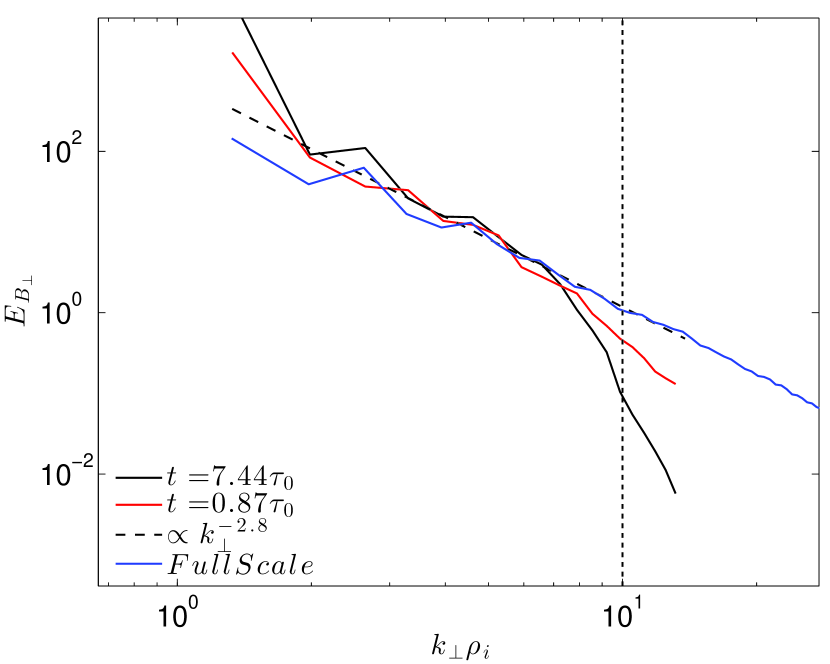
Figure 1: (Color online) Perpendicular magnetic energy spectra at the beginning (red) and end (solid black) of the frequency analysis compared to a larger, higher resolution simulation with similar plasma parameters (blue). The dashed line corresponds to a spectral slope of $-2.8$, and the vertical dotted line corresponds to the maximum fully resolved perpendicular scale.

III Critical Balance Theory

The strength of turbulence can be characterized by the ratio of the nonlinear cascade rate or perpendicular eddy turn-around time, $\omega_{nl}\simeq k_{\perp}v_{\perp}$, to the linear frequency,

$$\chi=\frac{\omega_{nl}}{\omega}=\frac{k_{\perp}v_{\perp}}{k_{\parallel}v_{A}}.$$ (4)

When $\chi\ll 1$, the turbulent fluctuations exist for several turn-around times at a given scale before their energy is cascaded to smaller scales—many wave-wave “collisions” are required to cascade their energy Iroshnikov (1963); Kraichnan (1965). This situation, known as weak turbulence Sridhar and Goldreich (1994), generates a cascade of energy in only the perpendicular direction Montgomery and Turner (1981); Shebalin et al. (1983). Therefore, $\chi$ grows with increasing perpendicular wavenumber, strengthening the nonlinear interactions. Once $\chi\simeq 1$, the timescales of the nonlinear and linear processes become equal, and the turbulence is said to be critically balanced Goldreich and Sridhar (1995, 1997).

It is interesting to consider also the over-strong case, $\chi\gg 1$. In this case, the nonlinear frequency is larger than the linear frequency, so two interacting Alfvén wave packets can undergo multiple cascades to smaller scales in a single linear crossing time. Therefore, the Alfvén wave packets are expected to be rapidly cascaded in the parallel direction until they restore the condition of critical balance, $\chi\simeq 1$. Note that fluctuations with $k_{\parallel}\simeq 0$, and therefore with $\omega\simeq 0$, are naturally generated by three-wave interactions of the Alfvénic turbulence Montgomery and Turner (1981); Goldreich and Sridhar (1995). This regime of over-strong turbulence is dominated by uncorrelated fluctuations, because fluctuations of scale $k_{\perp}$ are decorrelated over parallel distances greater then $k_{\parallel}\chi$. Thus, the energy in this over-strong region of wavenumber space is expected to be roughly constant, as observed in simulations of MHD turbulence Maron and Goldreich (2001).

The assumptions of critical balance and constant energy cascade rate lead to a predicted wavenumber anisotropy scaling of

$$k_{\parallel}\propto\begin{cases}k_{\perp}^{2/3},&{k}_{\perp}\rho_{i}\ll 1\\ k_{\perp}^{1/3},&{k}_{\perp}\rho_{i}\gg 1,\end{cases}$$ (5)

which can be combined into a single equation of the form

$${k}_{\parallel}\rho_{i}=(k_{i}\rho_{i})^{1/3}\frac{({k}_{\perp}\rho_{i})^{2/3}+({k}_{\perp}\rho_{i})^{\xi+2}}{1+({k}_{\perp}\rho_{i})^{2}},$$ (6)

where $\xi=1/3$ gives the standard dissipation range scaling derived from fluid theories assuming critical balance holds in the dissipation range Galtier (2006); Howes et al. (2008); Schekochihin et al. (2009). The form of Equation (6) has been chosen so that the asymptotic limits are continuously connected and it is well-behaved in its domain. Note that substituting Equation (6) into Equation (3) yields the linear Alfvén/KAW frequency $\omega$ in terms of only $k_{\perp}$.

A schematic diagram depicting the expected population of energy in critically balanced Alfvénic turbulence in terms of $\omega$ and $k_{\perp}$ is presented in Figure 2. The dispersion relation defines the critical balance boundary in the $k_{\perp}$-$\omega$ plane and corresponds to the solid line in Figure 2. Critical balance suggests the turbulent energy will fill the region below the critical balance boundary (shaded), as seen in inertial range MHD simulations of turbulence, e.g., Cho and Vishniac (2000); Maron and Goldreich (2001); Cho et al. (2002); Cho and Lazarian (2003); Oughton et al. (2004), and in dissipation range electron MHD simulations, e.g., Cho and Lazarian (2004, 2009).

Figure 2: Schematic diagram depicting the population of energy in the $k_{\perp}$-$\omega$ plane assuming critical balance holds. The solid lines correspond to the critical balance boundary. The isotropic energy injection scale is ${k}_{i}\rho_{i}=10^{-4}$.

To obtain a more realistic prediction of critical balance, we construct a physical model of the expected energy distribution. Previous models of critical balance, e.g., Goldreich and Sridhar (1995); Maron and Goldreich (2001), assume a form for the energy distribution in $k_{\perp}$-$k_{\parallel}$ space of $E(k_{\parallel},k_{\perp})\sim k_{\perp}^{-10/3}f(k_{\parallel}L^{1/3}/k_{\perp}^{2/3})$, where $f(|u|)\simeq 1$ for $u\leq 1$ and is negligibly small for $u\gg 1$.

We assume a similar functional form in $k_{\perp}$-$\omega$ space,

$$E(\omega,k_{\perp})=$$ (7)

$$E_{0}\frac{({k}_{\perp}\rho_{i})^{-\gamma-2/3}+({k}_{\perp}\rho_{i})^{-\epsilon+0.8}}{1+({k}_{\perp}\rho_{i})^{2}}\frac{1}{1+\left(\hat{\omega}/\hat{\omega}_{cb}\right)^{8}},$$

where $E_{0}$ is an overall energy normalization, $\gamma$ and $\epsilon$ are the desired inertial and dissipation range energy scalings, and $\hat{\omega}_{cb}=k_{\parallel}^{2}a_{0}\bar{\omega}/\sqrt{\beta_{i}}$. The functional form for the $k_{\perp}$ portion of Equation (7) is chosen empirically so that the frequency integrated energy reduces to a one-dimensional perpendicular energy spectrum that scales as $E_{B_{\perp}}(k_{\perp})=\int E(\omega,k_{\perp})\,d\omega\ \propto k_{\perp}^{-\gamma}$ in the inertial range and $k_{\perp}^{-\epsilon}$ in the dissipation range. We take $\gamma=5/3$ and $\epsilon=2.8$, consistent with the dissipation range solar wind Alexandrova et al. (2009) and large scale kinetic numerical simulations Howes et al. (2011). The functional form of the frequency has been chosen to have a flat energy spectrum up to $\sim\omega_{cb}$ followed by an $8$-th order roll-off at higher frequencies.

The logarithm of Equation  (7) is plotted in Figure 3a. Over plotted in Figure 3a is the linear frequency, which corresponds to the critical balance boundary. To make the boundary more clear, normalizing the energy at each $k_{\perp}$ by the zero frequency energy, $E(\omega,k_{\perp})/E(0,k_{\perp})$, yields Figure 3b.

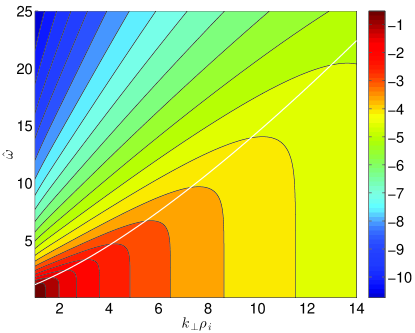
(a)

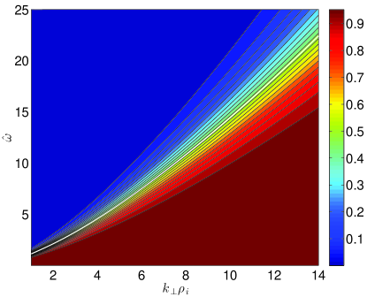
(b)

Figure 3: (Color online) (a) $\log{\left[E_{B_{\perp}}(\omega,k_{\perp})\right]}$ and (b) $E_{B_{\perp}}(\omega,k_{\perp})/E_{B_{\perp}}(0,k_{\perp})$, both computed based upon theoretical expectations. The white curve in both panels corresponds to the linear dispersion relation of kinetic Alfvén waves with $\xi=1/3$.

Since we have now constructed a more realistic numerical model of the critical balance energy distribution, given by Equation (7), we can examine the fraction of the turbulent energy falling below the critical balance boundary (in frequency) relative to the total energy at each $k_{\perp}$,

$$\frac{E}{E_{tot}}=\frac{\int_{\omega<\omega_{cb}}E(\omega,k_{\perp})\,d\omega\ }{\int E(\omega,k_{\perp})\,d\omega\ }.$$ (8)

This fraction is plotted as the solid line in Figure 4. Up to the point where finite box size limitations become important, $\simeq 90\%$ of the energy lies below the critical balance boundary.

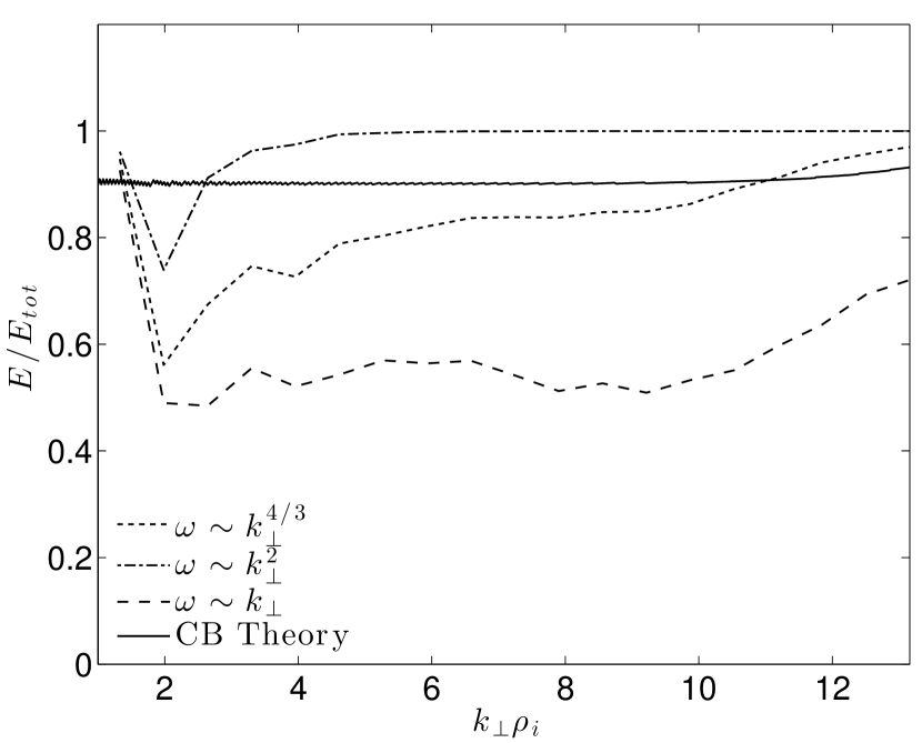
Figure 4: The fraction of energy beneath the critical balance boundary at each $k_{\perp}$. The solid line is based upon theoretical considerations of critical balance, while the other three curves are calculated from the AstroGK simulation with different values of $\xi$.

IV Critical Balance Simulation

We may now compare the energy distribution in $k_{\perp}$-$\omega$ space from the theoretical model for critical balance, given by Equation (7), with that determined through frequency analysis of our kinetic Alfvén wave turbulence simulation using AstroGK.

In Figure 5a is plotted the logarithm of the perpendicular magnetic energy. The figure was constructed by integrating the 3D AstroGK data in $k_{z}$ and annular sections in the $k_{x}$-$k_{y}$ plane. The over-plotted curves (black) correspond to critical balance with $\xi$ in Equation  (6) set to $0$ (dashed), $1/3$ (solid), and $1$ (dot-dashed), where $\xi=1/3$ is the conventional prediction for critically balanced kinetic Alfvén wave turbulence in the dissipation range.

Below the $\xi=1/3$ (solid black) critical balance boundary in Figure 5a, we find excellent qualitative agreement with the theoretical prediction represented in Figure 3a. Although the agreement is slightly poorer above this boundary, the fraction of the energy in this region is very small. The energy fraction falling below each of the curves in Figure 5a is plotted in Figure 4. The upward trend beginning at $k_{\perp}\rho_{i}\simeq 8$ is due to hypercollisionality and finite box size limitations, and the poor agreement at small $k_{\perp}$ is due to the effect of driving. Away from these limiting values, the difference between the theory and the simulation for $\xi=1/3$ is within approximately $10\%$.

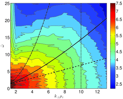
(a)

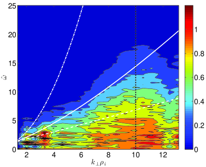
(b)

Figure 5: (Color online) (a) $\log{\left[E_{B_{\perp}}(\omega,k_{\perp})\right]}$ and (b) $E_{B_{\perp}}(\omega,k_{\perp})/E_{B_{\perp}}(0,k_{\perp})$ from the AstroGK simulation. The curves correspond to critical balance with $\xi=0,1/3,$ and $1$ in ascending order.

In Figure 5b is plotted the perpendicular magnetic energy at each $k_{\perp}$ normalized to the zero frequency energy, $E_{B_{\perp}}(\omega,k_{\perp})/E_{B_{\perp}}(0,k_{\perp})$. The figure was constructed in the same manner as Figure 5a, and the curves (white) correspond to the same values of $\xi$. As demonstrated with the theoretical model, plotting the energy distribution in $\omega$-$k_{\perp}$ space normalized in this fashion highlights the critical balance boundary, which closely follows the standard dissipation range prediction of $\xi=1/3$ (solid white). Again, the qualitative agreement with the prediction of critical balance is excellent. The non-smooth distribution of energy below the critical balance line in Figure 5b is primarily due to the discrete nature of this moderate resolution simulation.

Another method of visualizing the perpendicular magnetic energy distribution is to perform cuts along $\hat{\omega}$ at fixed $k_{\perp}$, as presented in Figure 6. Since the energy is plotted linearly, the area under each curve corresponds to the turbulent energy. Each panel of the figure represents a different $k_{\perp}$ slice, and the vertical dashed lines indicate the $\xi=1/3$ critical balance boundary. Panel a is influenced by the driving at $k_{\perp}\rho_{i}=1$, but it still displays similar qualitative behaviour to cuts at higher $k_{\perp}\rho_{i}$. The general trend can be seen to be an approximately flat energy distribution up to a frequency somewhat less than the critical balance boundary, followed by a steep roll-off. The majority of the energy in all cases is contained within the critical balance boundary. This plot makes clear an important characteristic of the turbulence: no energy significantly in excess of that predicted by the critical balance model is seen either at $\hat{\omega}=0$ or at frequencies above critical balance.

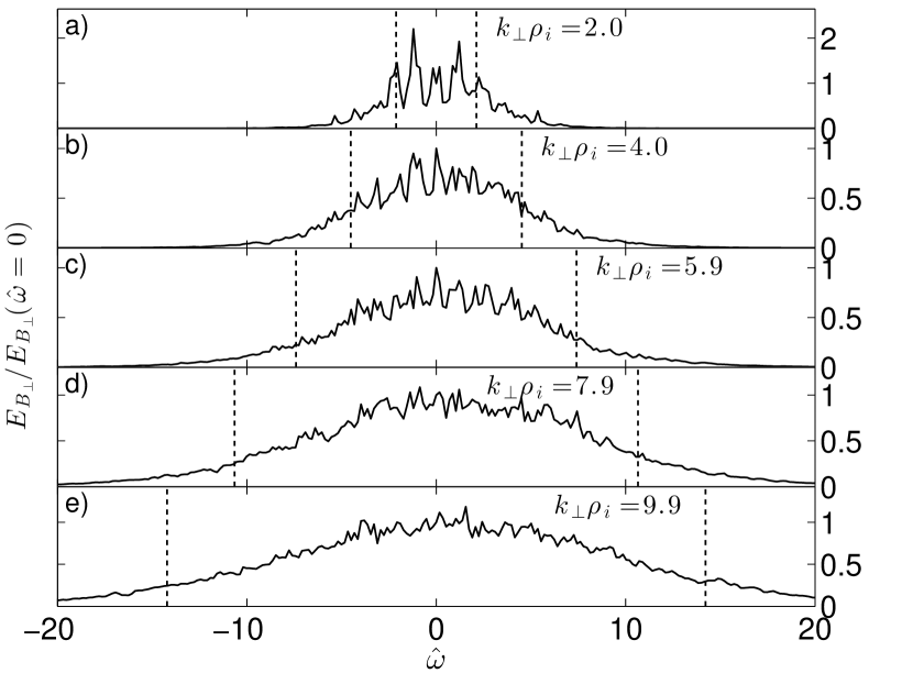
Figure 6: Perpendicular magnetic energy normalized to the zero frequency energy at each $k_{\perp}$ versus frequency at fixed $k_{\perp}$. The vertical lines represent the $\xi=1/3$ critical balance boundary. Panels a) - e) step through $k_{\perp}$ bins.

V Eulerian Frequency Analysis

Eulerian frequency spectra are constructed by placing an array of “probes” across a single spatial $x$-$y$ plane in the middle of the simulation domain. We use an array of $64\times 64$ probes across the plane to record a time series of the fluctuating magnetic field components. A schematic of the probe distribution can be seen in Figure 7.

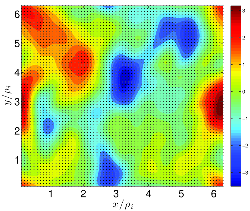
Figure 7: (Color online) $E_{B_{x}}$ at a single $z$ plane in the middle of the simulation domain. Overlaid are the positions of the “probes” used to record temporal fluctuations.

The evolution in time of the three magnetic field components at a single probe location over the same time interval used for the preceding critical balance study are illustrated in the upper panel of Figure 8. For illustrative purposes, over-plotted in the figure is $\cos{(t/\tau_{0}+0.5)}$. Clearly, the $B_{x}$ (blue) component is dominated by $\hat{\omega}\simeq 1$ fluctuations, which corresponds to the driving frequency and the lowest linear mode of the system.

In the lower panel of Figure 8 are plotted the Fourier response of the three magnetic field components averaged over the full probe array. All three magnetic field components are dominated by spectral peaks at $\hat{\omega}\simeq 0$ and $\pm 1$, with a clear band-gap between the values. As noted above, $\hat{\omega}\simeq\pm 1$ corresponds to the driving frequency and the lowest linear mode of the system. As such, this spectral component should contain the most power due to the driving, responsible for generating the forward cascade of energy to higher frequencies. We conjecture that the peak at $\hat{\omega}=0$ exhibits significant energy because this mode is responsible for nonlinear scattering in three-wave interactions of turbulence and is self-consistently generated via the nonlinear interaction Montgomery and Turner (1981); Sridhar and Goldreich (1994); Galtier and Bhattacharjee (2003).

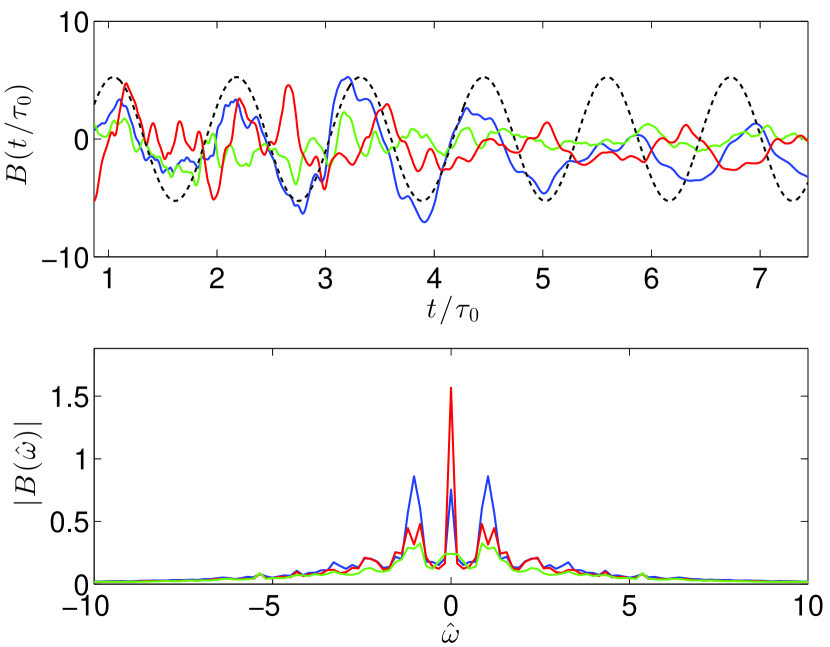
Figure 8: (Color online) In the upper panel is presented the temporal evolution at a single probe location of the three magnetic field components: $B_{x}$ (blue), $B_{y}$ (red), and $B_{z}$ (green). The dotted black line is $\cos{(t/\tau_{0}+0.5)}$. In the lower panel are presented the Fourier responses of the three magnetic field components averaged over the full probe array.

Figure 9 presents the Eulerian frequency spectrum of the perpendicular magnetic energy averaged over all probes. The vertical dotted lines indicate the minimum and maximum linear frequencies for the minimum and maximum resolved length scales in the simulation domain, as given by Equation (3). The frequency range around $\hat{\omega}\simeq 1$ is dominated by the antenna driving, so we fit from $\hat{\omega}=2$ to $14.4$ to obtain a spectral index of $\simeq-3.2$ for the Eulerian frequency spectrum.

Excluding the the driving dominated portion of the spectrum around $\hat{\omega}\simeq 1$, the energy in the low frequency range below $\hat{\omega}^{cb}_{min}$ is approximately constant, consistent with the predictions of critical balance outlined in §III. It is important to note that very little energy resides in these low frequency modes: the total integrated energy in the turbulence is the area under a linear plot of the frequency spectrum, so this low-frequency range corresponds to very little integrated area but is exaggerated in the logarithmically plotted Figure 9.

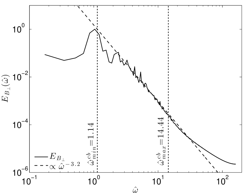
Figure 9: The perpendicular magnetic energy spectrum as a function of frequency averaged over the full probe array. The dashed line corresponds to a spectral index of $-3.2$. The vertical dotted lines correspond to the expected minimum and maximum frequencies from linear theory.

VI Discussion

The model for critical balance constructed in §III is based upon the theoretical expectations for strong turbulence, the foundation for which was established by Goldreich and Sridhar (1995): our model quantifies the qualitative arguments given therein and extends the notion of critical balance into the dissipation range, permitting arbitrary perpendicular wavevector scaling to agree with the results of large-scale kinetic numerical simulations Howes et al. (2011) and solar wind observations Alexandrova et al. (2009) of the dissipation range.

The theoretical model of critical balance is compared to our numerical simulations in §IV. Considering that the concept of critical balance is based upon order of magnitude scaling arguments, the agreement between theory and simulation presented in Figure 5b is striking. It is important to note that the nature of the energy input into our simulation domain generates perpendicular magnetic energy fluctuations that resemble linear Alfvén/KAWs. The turbulent fluctuations, however, are only driven at the smallest resolved wave numbers of our simulation domain, with the frequency range of the driving energy centered at $\hat{\omega}=\hat{\omega}_{0}$. Therefore, all of the energy at larger wave numbers and frequencies away from $\hat{\omega}_{0}$ results from self-consistent, nonlinear turbulent interactions.

The spectral anisotropy in fluid simulations is typically determined via two-point, second-order structure function analyses, e.g., Cho and Vishniac (2000); Maron and Goldreich (2001); Cho and Lazarian (2004); Chen et al. (2011). This approach allows one to identify the wavevector parallel to the local mean magnetic field at a given scale. A standard Fourier analysis provides only wavevectors parallel and perpendicular to the global mean magnetic field, i.e., $k_{z}$ and $k_{R}$, rather than $k_{\parallel}$ and $k_{\perp}$ Cho and Vishniac (2000); Maron and Goldreich (2001). This effect is a consequence of the inherent averaging of the Fourier transform. Turbulent fluctuations relevant to solar wind turbulence in the dissipation range are characterized by $\delta B_{\perp}/B_{0}\ll 1$ and $k_{\parallel}/k_{\perp}\ll 1$, so the Fourier transformed wavevector components are given, to lowest order, by $k_{R}\simeq k_{\perp}$ and $k_{z}\simeq\theta k_{\perp}$, where $\theta\simeq\delta B_{\perp}/B_{0}$ Maron and Goldreich (2001). Thus, a standard Fourier approach to analyzing turbulent simulations is sensitive only to the spectrum in $k_{\perp}$ and the amplitude of the fluctuating field, rather than $k_{\parallel}$ spectrum along the local mean magnetic field.

The structure function approach works well in MHD inertial range turbulence simulations and undamped dissipation range turbulence simulations, wherein the spectral slope is relatively shallow. The perpendicular spectra in kinetic simulations of dissipation range turbulence Howes et al. (2011) and in solar wind observations Alexandrova et al. (2009) have spectral indices around $-2.8$, and the parallel spectrum is expected to be steeper yet Cho and Lazarian (2004); Schekochihin et al. (2009); Chen et al. (2010). Two-point, second-order structure functions cannot recover spectral indices steeper than $-3$ Farge and Schneider (2006), and thus structure functions cannot be used to analyze the parallel spectrum of our dissipation range simulations.

The analysis performed herein obviates the limitations of structure function and spatial Fourier analyses by using the frequency $\omega$ as a proxy for $k_{\parallel}$. This approach is motivated by the fact that the linear frequency for the Alfvén and kinetic Alfvén wave is linearly proportional to parallel wavenumber, $\omega\propto k_{\parallel}$. This relation can be seen clearly by rewriting Equation (3) in the form $\omega(k_{\perp},k_{\parallel})=\overline{\omega}(k_{\perp})k_{\parallel}v_{A}$. The observation of a critical balance scaling in the turbulent energy distribution in $k_{\perp}$-$\omega$ space for our kinetic simulation of dissipation range turbulence implies that the spectral anisotropy observed in MHD inertial range simulations Cho and Vishniac (2000); Maron and Goldreich (2001); Cho et al. (2002); Cho and Lazarian (2003) and electron MHD dissipation range simulations Cho and Lazarian (2004, 2009) persists even in a turbulent kinetic plasma. Since the conventional critical balance boundary given by $\xi=1/3$ is a good fit to the turbulent energy distribution from our simulation, we conclude that the turbulent spectrum of kinetic Alfvén waves is well described by an anisotropic, critically balanced energy distribution in wavevector space given by $0<\xi\leq 1/3$, even for a fully nonlinear and collisionlessly damped kinetic simulation.

The results of §IV and V demonstrate that the theory of critical balance extends into the dissipation range of turbulence. Since critical balance is fundamentally a balancing of the linear and nonlinear processes in plasma turbulence, our results suggest that linear wave theory plays an important role, even in a strongly nonlinear turbulent plasma.

Dmitruk and Matthaeus (2009) (DM) performed a similar Eulerian frequency analysis of driven MHD turbulence, but their conclusions about the nature of the turbulence differ dramatically from our findings. In particular, they claim to find an excess accumulation of energy extending from their lowest linear mode to zero frequency and a very steep spectrum above their lowest linear mode. They conclude that linear waves play little role in MHD plasma turbulence. We believe the conclusions of DM are significantly biased by the set-up of their numerical simulations, for a number of reasons detailed below.

First, DM drive their simulations isotropically (with $k_{\perp}\sim k_{\parallel}$ for the driven modes) with a fixed amplitude, yielding a turbulent fluctuation amplitude $\delta B\sim 1$, for a range of values of the mean field strength $B_{0}=0,1,2,8,16$. The nonlinearity parameter for Alfvénic turbulence may be expressed as $\chi=k_{\perp}\delta B/k_{\parallel}B_{0}$, so the only case that yields strong MHD turbulence with $\chi\sim 1$ is the $B_{0}=1$ case; all other cases correspond to simulations of weak turbulence, with increasingly small nonlinearity parameters, $\chi=1/2,1/8,1/16$. That the turbulence is indeed weak is supported by the very steep spectral indices of their frequency spectra.

The nonlinear frequency in the weak turbulence regimeMaron and Goldreich (2001); Howes et al. (2011) is given by $\omega_{nl}\simeq\chi^{2}k_{\parallel}v_{A}$ , which suggests that one may expect to see a signature in the frequency spectrum corresponding to this very low nonlinear frequency, as indeed observed by DM. In addition, DM report that their simulations require “tens of nonlinear times” to reach a saturated steady state, although they do not define what they mean by a “nonlinear time.” If nonlinear time is taken to mean the Alfvén crossing time, their result is consistent with the expectation that it will take approximately one full nonlinear timescale, $\tau_{nl}\simeq\tau_{A}/\chi^{2}$, or many Alfvén crossing times, $\tau_{A}=2\pi/k_{\parallel}v_{A}$, to reach the steady state of the weak turbulent cascade. Note that other simulations of driven, strong MHD turbulence report the establishment of a steady state within one to a few Alfvén times, as expected for $\chi\sim 1$ Biskmap et al. (1999); Cho and Vishniac (2000); Cho and Lazarian (2004, 2009); Perez and Boldyrev (2010). Therefore, we speculate that the excess energy at low frequency observed in the weak turbulence simulations of DM may be attributed either to the response of the plasma at the low nonlinear frequency or to the inclusion, in the interval used for the frequency analysis, of the long transient evolution of the turbulence as it approaches a steady state.

Second, in weak turbulence, the resonant matching conditions for the nonlinear term in wavevector and frequency Shebalin et al. (1983); Sridhar and Goldreich (1994) for the dominant three wave interactions Montgomery and Matthaeus (1995); Ng and Bhattacharjee (1996); Goldreich and Sridhar (1997); Galtier et al. (2000); Galtier and Bhattacharjee (2003) imply a crucial role for modes with $k_{\parallel}=0$ in the nonlinear transfer of energy. According to the linear dispersion relation for Alfvén waves, $\omega=\pm k_{\parallel}v_{A}$, a fluctuation with $k_{\parallel}=0$ also has $\omega=0$. If such modes are generated by the nonlinear interactions in the turbulence, this could be another possible cause for an excess of energy in their frequency spectra at $\omega\simeq 0$.

Third, DM report that the frequency spectrum of their driving has the form $P(\omega)\sim 1/(\omega^{2}+\omega_{c}^{2})$, with $\omega_{c}=3$ in their dimensionless units. The antenna power therefore scales $P\propto\omega^{0}$ for $\omega\ll\omega_{c}$ and $P\propto\omega^{-2}$ for $\omega\gg\omega_{c}$. However, DM do not present a plot of the frequency spectrum of their driving, making it difficult to assess fairly the impact of the driving on the frequency spectra of their turbulence simulations. Since the parallel energy spectrum of strong MHD turbulence Howes et al. (2011) is predicted to scale as $E(k_{\parallel})\propto k_{\parallel}^{-2}$, the linear relationship between the parallel wavenumber and frequency implies a frequency spectrum $E(\omega)\propto\omega^{-2}$. In weak turbulence, the frequency spectrum would be steeper yet. Therefore, it is questionable whether one could observe even the strong turbulent frequency spectrum in the presence of their driving.

One may attempt to judge the impact of the driving by examining Figure 8 in DM, a comparison of the frequency spectra from a driven and an undriven simulation. It is important to note that both are weak turbulence simulations, so the contribution to the spectra due to the nonlinear turbulent fluctuations should be similar. The driven simulation shows a significantly larger signal over the frequency range $0.4\leq\omega\leq 10$, suggesting that the driving has a significant, if not dominant, effect on the frequency spectrum over this range. DM attribute the broadband nature of the frequency spectra in their suite of simulations, presented in their Figure 2, to the inherently nonlinear nature of MHD turbulence. We suggest that a more careful evaluation of the impact of their driving on the frequency spectrum is required to establish the validity of their conclusion.

We believe the arguments outlined above raise serious questions about the conclusions that DM reach regarding the nature of MHD turbulence, in particular the claim that linear mode properties play little role in the turbulent evolution. The concept of critical balance implicitly assumes that linear wave modes do play a role in plasma turbulence. The numerical evidence presented here for critical balance in the kinetic Alfvén wave cascade of dissipation range turbulence therefore indirectly supports the notion that linear wave modes do indeed play a role in strong plasma turbulence.

VII Conclusion

We have developed a theoretical model for critically balanced Alfvén/KAW turbulence and compared the results of a fully nonlinear, driven, gyrokinetic simulation to the theoretical prediction. We find excellent qualitative and quantitative agreement with the predictions of critical balance in the dissipation range of KAW turbulence. This result constitutes the first evidence of critical balance to be observed in a damped and dissipative kinetic turbulence simulation.

Having found agreement with critical balance implies the anisotropic cascade of Alfvén waves in the inertial range extends into the dissipation range, where the anisotropic scaling of KAW turbulence is observed to be approximately $k_{\parallel}\propto k_{\perp}^{\xi}$ with $0<\xi\leq 1/3$. The upper bound of this result agrees with theoretical predictions for the dissipation range scaling based upon fluid descriptions, and the damping present in our kinetic simulation is expected to strengthen the anisotropy Howes et al. (2011).

The results of our Eulerian frequency analysis performed by temporally sampling the magnetic field data across a fixed $x$-$y$ plane provide further evidence of a critically balanced cascade of energy beginning at our driving frequency. Aside from the expected population of energy in the $\omega=0$ mode, we find no evidence of excess energy either below the lowest or above the highest linear modes resolved in our simulation, in contradiction to Dmitruk and Matthaeus (2009).

Although the current analysis does not directly address the importance linear wave theory to plasma turbulence, agreement with critical balance implies linear wave modes play some role in governing turbulence. Forthcoming simulation analyses will explore the importance of linear wave modes in fully developed, strong plasma turbulence in more detail.