Measurements of the Cosmic Ray Composition with Air Shower Experiments

Abstract

In this paper we review air shower data related to the mass composition of cosmic rays above $10^{15}$ eV . After explaining the basic relations between air shower observables and the primary mass and energy of cosmic rays, we present different approaches and results of composition studies with surface detectors. Furthermore, we discuss measurements of the longitudinal development of air showers from non-imaging Cherenkov detectors and fluorescence telescopes.

The interpretation of these experimental results in terms of primary mass is highly susceptible to the theoretical uncertainties of hadronic interactions in air showers. We nevertheless attempt to calculate the logarithmic mass from the data using different hadronic interaction models and to study its energy dependence from $10^{15}$ eV to $10^{20}$ eV .

1 Introduction

Knowledge of the mass composition of cosmic rays is of key importance for solving the long standing puzzle about the origin of high-energy cosmic rays. The mass (and therefore charge) distribution can provide strong constraints on the acceleration of cosmic rays and on their propagation through the galactic and extragalactic Universe. Of particular interest are measurements of the mass composition in vicinity of structures observed in the energy spectrum of cosmic rays, most prominently the “knee” and the “ankle” at approximately $10^{15.5}$ eV and $10^{18.5}$ eV , respectively, as well as at energies above $10^{19.5}$ eV at which a flux suppression — possibly the GZK-effect — has been observed. Correlated changes of the energy spectrum and mass composition can provide important clues to the origin of these features. For instance, a rigidity dependent cut-off [1] of the spectra of cosmic rays with different charge can lead to a gradual increase in the average mass of galactic (see [2] and references therein) and extra-galactic cosmic rays [3, 4, 5]. On the other hand, the interpretation of the ankle and flux suppression as a signature of propagation effects [6, 7] of ultra-high energy extragalactic protons would require a very light composition above the ankle [8]. Furthermore, the location and nature of the transition from galactic to extragalactic cosmic rays (or lack thereof [9]) leads to distinct predictions of the energy evolution of the mass composition of cosmic rays in the energy region between $10^{17}$ eV and $10^{19}$ eV (see e.g. [10, 11, 12, 13, 14, 15]).

Up to energies of some $10^{14}$ eV , the cosmic ray composition can be measured directly and with only minor, or none disturbing effects from cosmic ray interactions in the atmosphere, by employing stratospheric balloon- or satellite-borne experiments, respectively. Cosmic rays at these energies are covered elsewhere, see e.g. [16] or [17] and [18] in this volume. At higher energies, measurements of cosmic rays are only possible via observations of extensive air showers (EAS). Amongst all EAS measurements, those aiming at reconstructing the cosmic ray mass composition are the most difficult ones. This is, because the mass of the primary particle can only be inferred from detailed comparisons of experimental observables with air shower simulations, with the latter being subject to uncertainties of hadronic interactions at the highest energies. Fortunately, the data from the LHC at CERN will allow for detailed tests of interaction models up to center of mass energies being equivalent to cosmic ray energies of $10^{17}$ eV , but an appreciable amount of extrapolation of the properties of hadronic interactions will still be needed to interpret the air shower data up to energies of $10^{20}$ eV . In fact, these model uncertainties become a dominant source of systematics of estimates of the cosmic ray mass composition at the highest energies. Therefore, identifying different EAS observables with sensitivity to the primary mass is of great importance as these different observables should lead to consistent conclusions about the properties of the primary particles. Inconsistent conclusions, on the contrary, would be indicative for deficiencies of the employed hadronic interaction models.

High energy photons and neutrinos can provide an indirect approach to the composition of cosmic rays at the highest energies. This is because photo-pion production via the Greisen-Zatsepin-Kuzmin effect [6, 7] leads to emission of neutrinos [19] and photons from pion decays in the reactions $p+\gamma_{\mathrm{CMB}}\to p+\pi^{0}\to p+\gamma\gamma$, or likewise $p+\gamma_{\mathrm{CMB}}\to n+\pi^{+}\to n+\mu^{+}+\nu_{\mu}\to n+e^{+}+\nu_{e}+\bar{\nu}_{\mu}+\nu_{\mu}$. The discovery of cosmogenic photons and neutrinos would prove the existence of the GZK energy loss mechanism independently from the cut-off in the cosmic ray energy spectrum and would be the unambiguous consequence of a light cosmic ray composition at ultra-high energies. In the case of heavy primaries, the photo-pion production sets in at much higher energies, because the energy threshold for this reaction depends on the energy per nucleon and not the total energy. Instead, photo-disintegration is the dominant process [20] for energy losses, giving rise to neutrinos from neutron decays, but yielding much lower neutrino fluxes in the EeV range compared to the photo-pion production by primary protons.

This paper is organized as follows: In the next section we will provide an overview of the most important air shower observables with respect to measurements of the nuclear composition. In Sec. 3 experimental results covering the energy range from the knee to ultra-high energies will be presented and searches for high energy photons and neutrinos will be briefly discussed in Sec. 4. In this review we focus on measurements of the cosmic ray composition from air shower experiments only. Other aspects of cosmic rays above the knee are discussed elsewhere in this volume [21, 22, 23] and in [24, 25, 26, 27].

2 Air Shower Observables Sensitive to Composition

There exist a plethora of experimental techniques to characterize air shower features. In the context of mass composition at least two orthogonal measurements are needed to estimate both, the energy and mass, of the primary cosmic ray that initiated the EAS. This is usually achieved by observing either the longitudinal development of a shower or by the simultaneous determination of the electromagnetic and muonic component of EAS at ground level. Further insights can be gained by the study of the lateral distribution of particles at ground level, which is related to the longitudinal development stage of the shower at observation level.

The ability to deduce the nuclear composition of cosmic rays on a statistical basis from these measurements relies to a large extent on the theoretical understanding of the shower development and the hadronic interactions that occur within the cascade. However, the major differences between air showers induced by different primary masses have a rather simple cause. The discriminating power originates from the fact that a primary nucleus of mass $A$ and energy $E$ can in good approximation be treated as a superposition of $A$ nucleons of energy $E^{\prime}=E/A$. This superposition model seems plausible because the binding energy of nucleons is much smaller than the energy of the primary particle. However, the nucleons of a primary nucleus are obviously not independent. For instance, the first interaction of a nucleus of mass $A$ will happen on average at a depth $\langle X_{\mathrm{first}}\rangle$ equal to the interaction length $\lambda_{A}<\lambda_{p}$ and the average number of nucleons participating in the first interaction, $\langle n_{A}\rangle$, fluctuates. Interestingly enough, it can be shown [28] that for $\langle n_{A}\rangle=A\,\lambda_{A}/\lambda_{p}$ (the average number of participating nucleons from Glauber theory [29]), the inclusive distribution of first interactions follows exactly the expectation of the naive superposition model, namely that the average depth of interaction of the $A$ nucleons is $\lambda_{p}$. This is the semi-superposition theorem that provides a justification of the superposition ansatz under more realistic assumptions.

Whereas the superposition model can explain the main differences between air showers induced by different nuclei, it does of course not account for nuclear effects such as re-interaction in the target nucleus or for the effect of nuclear fragmentation on air shower fluctuations (see e.g. [30, 31, 32]). More realistic predictions of air showers can be obtained by using transport codes like Corsika [33], Aires [34] or Cosmos [35] together with hadronic interactions models such as Epos [36], QGSJet [37] or Sibyll [38] (see [39] for a comprehensive review of air shower simulations).

While these transport codes can give an accurate description of air showers given a model for hadronic interactions, it is often desirable to qualitatively understand the basic physics behind a certain air shower observable. For this purpose it can be constructive to calculate the air shower development within the Heitler-model [40, 41] in which the cascade is approximated by a simple deterministic branching model. The original treatment of electromagnetic cascades has recently been extended to hadronic showers in [42, 43, 44] and some of these qualitative dependencies will be referred to in the following.

2.1 Longitudinal Development

The observation of the longitudinal development of the particle cascade in the atmosphere is especially well suited for composition studies. In analogy to particle physics detectors, the atmosphere acts as a huge homogeneous (as opposed to sampling) calorimeter in which the air is both the passive material that drives the shower development and the active material that allows the detection of the produced particles via fluorescence or Cherenkov light (cf. Sec. 3.2 and 3.3), as well as the light guide through which the signal is transferred to the detector.

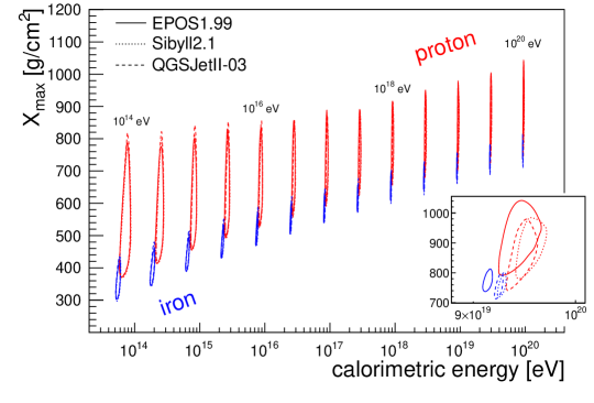
Figure 1: Air shower simulation of the shower maximum vs. calorimetric energy. Contour lines illustrate the regions which include 90 % of the showers and the inset shows a detailed view at $10^{20}$ eV .

The first inelastic interaction of the primary particle of energy $E$ and mass $A$ with an atmospheric nucleus occurs at an average depth which is equal to interaction length for inelastic nucleus-air collisions, $\lambda_{A-\mathrm{air}}$. In this and each consecutive interaction about one third of the primary energy is transferred from the hadronic to the electromagnetic component of the shower via decays of neutral pions into photons. The energy transfer continues until the charged hadrons decouple from the shower by decay into muons and neutrinos, i.e. until their interaction length becomes larger than their decay length (see next section). If the charged hadrons start to decay on average after $n_{\mathrm{d}}$ interaction lengths, then the energy in the electromagnetic component is

$$E_{\mathrm{cal}}\approx E\left(1-\left(\frac{2}{3}\right)^{n_{\mathrm{d}}}\right).$$ (1)

Since $n_{\mathrm{d}}\geq 5$ for energies $\geq$$10^{15}$ eV  [45], it follows that most of the energy of an air shower can be observed in its electromagnetic part and it is this so-called calorimetric energy which allows detectors that can observe the longitudinal air shower development to estimate the primary energy with good accuracy.

Given this estimator of the energy of the primary particle, the orthogonal variable sensitive to its primary mass is the slant depth at which the particle cascade reaches its maximum in terms of the number of particles, ${X_{\mathrm{max}}}$. This shower maximum is dominated by electromagnetic sub-showers produced in the interaction with the largest inelasticity which is usually (though not always) the first interaction. An electromagnetic shower of energy $E$ reaches its maximum at about

$$\langle X_{\mathrm{max}}^{\mathrm{emag}}\rangle\approx X_{0}\ln{E/\varepsilon_{\mathrm{c}}^{\mathrm{em}}}$$ (2)

where $X_{0}\approx 36.62$ g/cm² is the radiation length in air and $\varepsilon_{\mathrm{c}}^{\mathrm{em}}\approx 84$ MeV is the critical energy in air at which ionization and bremsstrahlung energy losses are equal. If the total multiplicity of hadrons produced in the main interaction is $N$ and the average hadron energy is $E/N$, then the shower maximum of a primary proton is

$$\langle X_{\mathrm{max}}^{p}\rangle\approx\lambda_{p}+X_{0}\ln\left(\frac{E}{2N\varepsilon_{\mathrm{c}}^{\mathrm{em}}}\right)$$ (3)

where both the hadronic interaction length and particle production multiplicity are energy dependent. The factor 2 takes into account that neutral pions decay into two photons. Furthermore, the shower maximum is expected to be influenced by the elasticity of the first interaction, $\kappa_{\mathrm{ela}}=E_{\mathrm{lead}}/E$, where $E_{\mathrm{lead}}$ is the energy of the highest energy secondary produced in the interaction. For interactions with $\kappa_{\mathrm{ela}}>0.5$ most of the primary energy will be transferred deeper into the atmosphere and correspondingly the shower maximum will be deeper. We are not aware of a consistent treatment of the elasticity within a Heitler model for the longitudinal development, however using air shower simulations, the dependence on the elasticity fits well to

$$\langle X_{\mathrm{max}}^{p}\rangle\approx\lambda_{p}+X_{0}\ln\left(\frac{\kappa_{\mathrm{ela}}E}{2N\varepsilon_{\mathrm{c}}^{\mathrm{em}}}\right).$$ (4)

The elongation rate [46, 47, 48] is a measure of the change of the shower maximum per logarithm of energy,

$$D=\frac{\text{d}\langle X_{\mathrm{max}}\rangle}{\text{d}\ln E}.$$ (5)

For protons and constant elasticity Eq. (4) gives

$$D_{\mathrm{p}}=\frac{\mathrm{d}\langle X_{\mathrm{max}}^{p}\rangle}{\mathrm{d}\ln E}\approx X_{0}\,(1-B_{N}-B_{\lambda})$$ (6)

where the changes in multiplicity and interaction length are given by

$$B_{N}=\frac{\mathrm{d}\ln N}{\mathrm{d}\ln E}\quad\mathrm{and}\quad B_{\lambda}=-\frac{\lambda_{p}}{X_{0}}\frac{\mathrm{d}\ln\lambda_{p}}{\mathrm{d}\ln E}.$$ (7)

Since hadronic interaction models predict an approximately logarithmic decrease of $\lambda_{p}$ with energy and $N\varpropto E^{\delta}$, $D_{p}$ is approximately constant and therefore

$$\langle X_{\mathrm{max}}^{p}\rangle\approx c+D_{p}\ln E,$$ (8)

with parameters $c$ and $D_{\mathrm{p}}$ being dependent on the characteristics of hadronic interactions. Using the aforementioned (semi-)superposition assumption, one obtains

$$\langle X_{\mathrm{max}}^{A}\rangle=\langle X_{\mathrm{max}}^{p}(E^{\prime}=E/A)\rangle=c+D_{p}\ln(E/A)$$ (9)

and at a given energy the average shower maximum for a mixed composition with fractions $f_{i}$ of nuclei of mass $A_{i}$ is

$$\langle X_{\mathrm{max}}\rangle\approx\sum_{i}f_{i}\,\langle X_{\mathrm{max}}^{A_{i}}\rangle=\langle X_{\mathrm{max}}^{p}\rangle-D_{p}\,\langle\ln A\rangle.$$ (10)

This equation explicitly demonstrates the relation of ${\langle X_{\mathrm{max}}\rangle}$ to the average logarithmic mass of the cosmic ray composition, $\langle\ln A\rangle=\sum_{i}f_{i}\,\ln A$.

The numerical value of $D_{p}$ from air shower simulations is about 25 g/cm² (or about 60 g/cm² for the change in ${\langle X_{\mathrm{max}}\rangle}$ per decade, $D_{10}^{p}=\ln(10)\,D_{p}$) and therefore proton and iron induced air showers are expected to differ by around $D_{p}(\ln 56-\ln 1)\approx 100\,{\mathrm{g/cm}^{2}}$. Moreover, if the hadronic cross sections and multiplicities rise with energy (and if there are no sudden changes in the elasticity as for instance suggested in [49]), then Eq. (7) leads to Linsley’s elongation rate theorem which states that the value of $D_{p}$ cannot exceed the radiation length in air, $X_{0}$. Therefore, Eq. (10) implies that if an experiment measures an elongation rate of $D>X_{0}$, then a change in the cosmic ray composition from light to heavy, $\text{d}\langle\ln A\rangle/\text{d}\ln E>0$, must be responsible for that larger value.

Results of air shower simulations of $\langle X_{\mathrm{max}}\rangle$ and $E_{\mathrm{cal}}$ are shown in Fig. 1. As can be seen, the calorimetric energy is indeed a good proxy for the primary energy and exhibits only small shower-to-shower fluctuations. And, as expected from the relations sketched above, the shower maximum penetrates deeper into the atmosphere with the logarithm of the energy and is shallower for heavy nuclei than for light ones. The shower-to-shower fluctuations in $X_{\mathrm{max}}$ are however large and even extreme compositions like pure proton vs. pure iron have a considerable overlap in their ${X_{\mathrm{max}}}$-distributions.

However, these fluctuations carry interesting information about the primary particle types and/or the ’mixedness’ of the cosmic ray composition, that can be experimentally exploited. For protons the standard deviation $\sigma$ of the ${X_{\mathrm{max}}}$-distribution, $\sigma^{2}=\langle(X_{\mathrm{max}}^{p})^{2}\rangle-\langle X_{\mathrm{max}}^{p}\rangle^{2}$, is given by the quadratic sum of the fluctuation of the first interaction point and the fluctuations of the shower development, which in case of the simple Heitler model Eq. (4) reduces to

$$\sigma^{2}_{p}\approx\lambda_{p}^{2}+\left(X_{0}\frac{\sigma(N)}{N}\right)^{2}+\left(X_{0}\frac{\sigma(\kappa_{\mathrm{ela}})}{\kappa_{\mathrm{ela}}}\right)^{2}.$$ (11)

Interestingly, for a geometrical treatment of nucleus-nucleus scattering [50], the relative fluctuations of the multiplicity, $\sigma(N)/N$, are constant. Furthermore, if the relative fluctuations of the elasticity do not depend on energy, then $\sigma^{2}_{p}$ is expected to decrease with energy reflecting the logarithmic rise of the proton-air cross section.

For primary nuclei, the naive expectation from the superposition model would be $\sigma_{A}=\sigma_{p}/\sqrt{N}$. As will be seen in Fig. 11, air shower simulations predict a $\sigma_{p}$ of about 60 g/cm² at $10^{18}$ eV and correspondingly $\sigma_{\mathrm{Fe}}$ should be at the level of 8 g/cm² whereas a much larger value of $\approx 20$ g/cm² is predicted. The reason for this discrepancy is that although according to the semi-superposition theorem the positions of elementary nucleon-nucleon interactions are distributed $\varpropto\exp(-X/\lambda_{p})$, the individual positions are not independent. For instance, the $n$ nucleons participating in the first interaction have all the same $X=X_{\mathrm{first}}$. These correlations together with the event-by-event variance of $n$ are the main reason for $\sigma_{A}>\sigma_{p}/\sqrt{N}$. In addition there are two extreme cases for the spectator nucleons: Either complete fragmentation (i.e. all $A-n$ spectators propagate independently after $X_{\mathrm{first}}$) or a single spectator nucleus with $A^{\prime}=A-n$, where the latter case without fragmentation would result to an additional broadening of the ${X_{\mathrm{max}}}$-distribution.

In the interesting case of a mixed composition with fractions $f_{i}$ of nuclei of mass $A_{i}$, the combined ${X_{\mathrm{max}}}$-distribution follows from elementary statistics [51]. If each component has an average shower maximum of ${\langle X_{\mathrm{max}}\rangle}_{i}$ with width $\sigma_{i}$ then

$$\sigma({X_{\mathrm{max}}})^{2}=\langle\sigma_{i}^{2}\rangle+\left(\left\langle{\langle X_{\mathrm{max}}\rangle}_{i}^{2}\right\rangle-{\langle X_{\mathrm{max}}\rangle}^{2}\right)$$ (12)

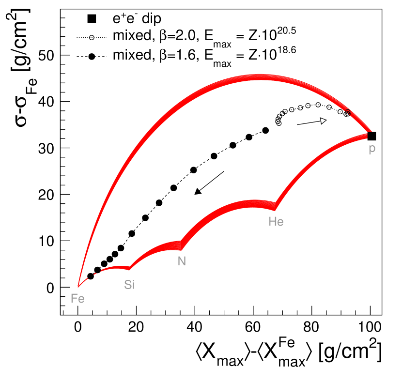
Figure 2: Composition sensitivity of a combined measurement of the shower maximum and its fluctuations. Dots denote different models of the extragalactic cosmic ray composition at Earth: Pure proton composition in the dip-model [8] and mixed composition with a large [11] or small [23] maximum energy of the sources and different spectral indices $\beta$ at the source. Energies range from $10^{18.5}$ eV to $10^{20}$ eV with a spacing of $\Delta\lg E=0.1$. Red lines are simulations with Sibyll at the same energies for various two-component transitions. The contour defined by these transition contains all other possible mixtures for $1\leq A\leq 56$.

where ${\langle X_{\mathrm{max}}\rangle}=\left\langle{\langle X_{\mathrm{max}}\rangle}_{i}\right\rangle$ is the mean of the combined distribution. In case of a composition comprised of two components only, this reduces to

$$\sigma({X_{\mathrm{max}}})^{2}=f\sigma_{1}^{2}+(1-f)\,\sigma_{2}^{2}+f(1-f)(\Delta{\langle X_{\mathrm{max}}\rangle})^{2}.$$ (13)

Therefore, depending on the separation of the mean values $\Delta{\langle X_{\mathrm{max}}\rangle}$ and the fraction $f$ of component $1$, it can happen that the combined distribution is broader than the individual distributions because their separation adds to the total width. In terms of average logarithmic mass, Eq. (12) can be rewritten as

$$\sigma({X_{\mathrm{max}}})^{2}=\langle\sigma_{i}^{2}\rangle+D_{p}^{2}\left(\langle\ln^{2}A\rangle-{\langle\ln A\rangle}^{2}\right),$$ (14)

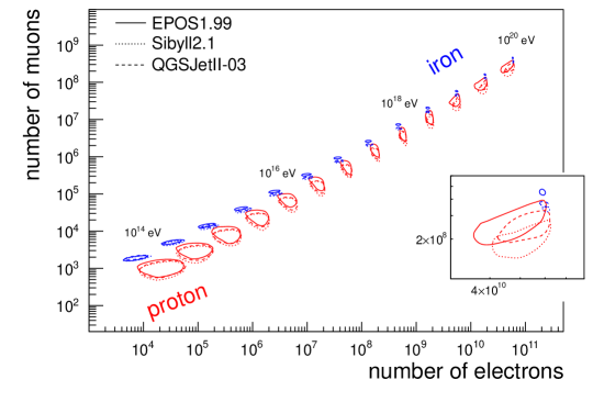
Figure 3: Air shower simulation of the number of muons vs. electrons at ground level for a vertical shower observed at 800 g/cm². Contour lines illustrate the regions which include 90 % of the showers and the inset shows a detailed view at $10^{20}$ eV .

which demonstrates that $\sigma({X_{\mathrm{max}}})^{2}$ is proportional to the variance of $\ln A$. Starting from this equation, Linsley proposed to analyze air shower data in the $\sigma(\ln A)-{\langle\ln A\rangle}$ plane [52] which, however, involves the need to specify the dependence of $\sigma_{A}$ on $\ln A$. In this article we will use a similar approach below (cf. Sec. 3.3), but stick to the experimental $\sigma({X_{\mathrm{max}}})$ and ${\langle X_{\mathrm{max}}\rangle}$ values. For the purpose of comparing data at several energies to model predictions, it is useful to subtract the (energy dependent) values for iron nuclei from both the data and predictions. The approximate energy independence of this subtracted variables is illustrated in Fig. 2. Two-component transitions as predicted from air shower simulations with Sibyll are shown as curves that are, as expected from Eq. (13), parabolas in the $\sigma({X_{\mathrm{max}}})$-${\langle X_{\mathrm{max}}\rangle}$ plane. These parabolas define a closed contour that contain all possible combinations of mass mixtures for $A\in[1,56]$. To illustrate the discriminative power of the $\sigma({X_{\mathrm{max}}})$-${\langle X_{\mathrm{max}}\rangle}$ combination, three models for energy evolution of the extragalactic cosmic ray composition [8, 11, 23] are shown as well.

2.2 Particles at Ground

Another way of detecting cosmic rays and to estimate their mass is given by the measurement of particle densities of air showers at ground. In the calorimeter analogy of the previous section, this would correspond to a calorimeter with only one active readout plane and correspondingly this measurement technique is more susceptible to shower-to-shower fluctuations. Nevertheless, ground measurements are still frequently used in cosmic ray detectors because of their geometric acceptance and high duty cycle.

An estimate of the qualitative dependencies of the number of muons and electrons on primary mass and characteristics of hadronic interactions can again be obtained within the Heitler model. Given the average multiplicity $N$ of each interaction, the energy of charged and neutral pions in a shower initiated by a primary proton of energy $E$ is $E_{\pi}=E/N^{n}$ after the $n$th interaction if one (somewhat unrealistically) assumes an energy independent multiplicity. This energy splitting continues until the charged pion energy reaches the decay energy at which the hadronic interaction length $\lambda_{\mathrm{int}}$ becomes equal to the decay length $\lambda_{\mathrm{dec}}=\rho\,\gamma\,c\tau$, where $\rho$ is the height-dependent density of air, $\gamma$ denotes the Lorentz-boost and $\tau$ is the pion lifetime. For a shower with incident angle $\theta$ in an isothermal atmosphere with scale height $h_{0}$, the density at slant depth $X$ is

$$\rho(h)=\frac{X}{h_{0}}\cos\theta=\frac{n\lambda_{\mathrm{int}}}{h_{0}}\cos\theta.$$ (15)

Therefore, the condition $\lambda_{\mathrm{int}}=\lambda_{\mathrm{dec}}$ leads to a decay energy that is independent of the interaction length. It is reached after $n_{\mathrm{d}}$ interactions for which

$$n_{\mathrm{d}}\,N^{-n_{\mathrm{d}}}=\frac{h_{0}}{c\tau}\frac{m_{\pi}\,c^{2}}{E}\frac{1}{\cos\theta}$$ (16)

and therefore

$$n_{\mathrm{d}}=-\frac{\mathrm{W}_{\kern-0.70004pt-1}\left(-\frac{h_{0}}{c\tau}\frac{m_{\pi}\,c^{2}}{E}\frac{\ln N}{\cos\theta}\right)}{\ln N},$$ (17)

where $\mathrm{W}_{\kern-0.70004pt-1}$ denotes the lower branch of the Lambert-W function (see e.g. [53]). The decay energy is then given by

$$\varepsilon_{\mathrm{d}}^{\pi}=\frac{E}{N^{n_{\mathrm{d}}}}$$ (18)

for which we find numerical values of a few tens of GeV and a slow decrease with primary energy in agreement with the estimates of [43]. The total number of muons produced in a shower is equal to the number of pions with $E_{\pi}=\varepsilon_{\mathrm{d}}^{\pi}$ and therefore

$$N_{\mu}^{p}\approx\left(\frac{E}{\varepsilon_{\mathrm{d}}^{\pi}}\right)^{\beta}$$ (19)

with

$$\beta=\frac{\ln\frac{2}{3}N}{\ln N},$$ (20)

where the factor $\frac{2}{3}$ gives the approximate fraction of charged pion secondaries. Air shower simulations predict $\beta$ to be in the range of 0.88 to 0.92 [42], corresponding to effective multiplicities from 30 to 200 in Eq. (20). It is interesting to note, that because the interaction length drops out in the calculation of $n_{d}$ (cf. Eq. (16)), the number of muons at ground are expected to be independent of $\lambda_{\mathrm{int}}$.

The number of electrons at shower maximum, i.e. at the point at which the electron energies become too low to produce new particles ($E_{e}=\varepsilon_{\mathrm{c}}^{\mathrm{em}}$), can be estimated from the total amount of energy in the electromagnetic cascade given by the primary energy minus the energy in muons. Since $E_{\mu}=N_{\mu}\varepsilon_{\mathrm{d}}^{\pi}$, the number of electrons is

$$N_{e,\mathrm{max}}^{p}=\frac{E}{\varepsilon_{\mathrm{c}}^{\mathrm{em}}}-\frac{\varepsilon_{\mathrm{d}}^{\pi}}{\varepsilon_{\mathrm{c}}^{\mathrm{em}}}\left(\frac{E}{\varepsilon_{\mathrm{d}}^{\pi}}\right)^{\beta}\approx\frac{E}{\varepsilon_{\mathrm{c}}^{\mathrm{em}}},$$ (21)

where the last approximation can be made at high energies at which the energy fraction transfered to muons becomes small.

Using again the superposition model and substituting $E$ with $E^{\prime}=E/A$, one obtains the following relations for nuclear primaries:

$$N_{e,\mathrm{max}}^{A}\approx A\frac{E/A}{\varepsilon_{\mathrm{c}}^{\mathrm{em}}}=N_{e,\mathrm{max}}^{p}$$ (22)

and

$$N_{\mu}^{A}\approx A\left(\frac{E/A}{\varepsilon_{\mathrm{d}}^{\pi}}\right)^{\beta}=N_{\mu,\mathrm{max}}^{p}\,A^{1-\beta}.$$ (23)

So, whereas the number of electrons at shower maximum gives a good estimate of the primary energy independent of the composition, the number of muons can be used to infer the mass of the primary particle, since it grows with $A^{1-\beta}$. Moreover, the evolution of the muon number with energy, $\mathrm{d}N_{\mu}/\mathrm{d}\ln E$, is a good tracer of changes in the primary composition. Just as in the case of the elongation rate of the longitudinal development, a constant composition gives $\mathrm{d}N_{\mu}/\mathrm{d}\ln E=\beta$ and any departure from that behavior can be interpreted as a change of the average mass of the primaries.

Unfortunately, the experimental situation is more complicated, because surface detectors do not observe the number of electrons at shower maximum, but at a fixed depth $X_{\mathrm{ground}}/\cos\theta$. If the detector and shower maximum are separated by $\Delta X=X_{\mathrm{ground}}/\cos\theta-{X_{\mathrm{max}}}$, then only the attenuated number of electrons is observed with

$$N_{e,\mathrm{ground}}\approx N_{e,\mathrm{max}}\,\exp{\left(-\frac{\Delta X}{\Lambda}\right)},$$ (24)

where $\Lambda\approx 60$ g/cm² is the attenuation length of the number of electrons after the shower maximum. Since heavy primaries reach their shower maximum at smaller depths than light ones, the number of electrons on ground is expected to be composition sensitive as well, with a larger electron number for air showers initiated by light primaries. This feature is visible in Fig. 3, where $N_{\mu}$ vs. $N_{e}$ is shown for air shower simulations at different energies for a detector located at 800 g/cm². As can be seen, the $\ln N_{\mu}$ and $\ln N_{e}$ observables are basically rotated from the desired quantities, $\ln A$ and $\ln E$. Due to the steeply falling cosmic ray spectrum, this rotation causes a complication in the analysis of air shower data, because showers of equal $\ln N_{e}$ are enriched in light elements (cf. Sec. 3.1 for a description of unfolding methods to overcome this problem). Furthermore, Eq. (24) implies that given the ${X_{\mathrm{max}}}$ fluctuations explained in the last section, the relative fluctuations of the electron number are expected to be quite substantial,

$$\frac{\sigma(N_{e,\mathrm{ground}})}{N_{e,\mathrm{ground}}}\approx\frac{\sigma({X_{\mathrm{max}}})}{\Lambda}.$$ (25)

These attenuation effects can be reduced considerably by choosing an appropriate detector site which is situated at a height close to the shower maximum. The exponential attenuation Eq. (24) is only valid far from the maximum, whereas in its close vicinity the shower size is nearly invariant under small displacements from the maximum (see Fig. 9 below). Since the simulations in Fig. 3 were performed at a fixed ground depth of 800 g/cm², the evolution of the attenuation effect with distance to the shower maximum can be seen indirectly: At low energies where the observation level is far from the shower maximum, the difference in the number of electrons between proton and iron primaries is large and diminishes while the shower maximum approaches the ground level at higher energies.

Besides the measurement of the number of electrons and muons, experiments with surface detectors have further means to determine the shower age (i.e. the distance to the shower maximum) by studying the shape of the particle densities with respect to the distance to the shower core. These measurements of the lateral distribution as well as other additional composition sensitive variables from ground detectors will be discussed in Sec. 3.1.2.

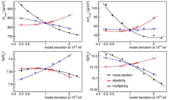
Figure 4: Sensitivity of air shower observables on characteristics of hadronic interactions as a function of a change in model characteristics growing logarithmically from zero at Tevatron energies to the quoted values on the x-axis at $10^{19}$ eV (proton showers at $10^{19.5}$ eV , adapted from [54]).

2.3 Model Uncertainties

The physics of air showers is very well understood in terms of particle transport through the atmosphere and for electromagnetic showers it is currently believed that they can be modeled without any significant uncertainties. In the case of hadronic showers, however, there is a fundamental lack of theoretical and experimental knowledge of the characteristics of hadronic interactions (see e.g. [55, 56] for recent discussions of hadronic interactions in air showers). Since most of the interactions in an air shower are ’soft interactions’, i.e. occur with only a small momentum transfer, perturbative QCD is not applicable. The phenomenological interaction models that have to be used instead, are constrained by low energy experimental data only, but even at these energies the full phase space relevant for air shower interactions is not fully covered [57, 58, 45, 59]. At ultra-high energies, the center of mass energies of the first nucleus-air interactions are beyond accelerator energies and correspondingly the models solely rely on extrapolations.

This somewhat bleak situation is currently alleviated by special-purpose programs to measure particle production data relevant for cosmic rays (e.g. [60, 61]) and by the wealth of new data from the multipurpose detectors at the LHC with which the interaction models can be tested and re-tuned. At its maximum center of mass energy of 14 TeV the LHC will eventually reach the equivalent of $10^{17}$ eV in the laboratory system and thus cover most of the energy range at which galactic cosmic rays are detected with air showers. First comparisons of the 7 TeV data to interaction models used in air shower simulations suggest that the LHC data are bracketed by these models [62].

The effect of uncertainties in hadronic interaction characteristics on air shower observables has been recently studied in [54] and [63]. Some of the results from [54] are displayed in Fig. 4 where response of air shower observables to ad-hoc changes of the Sibyll interaction model are shown. As can be seen, all air shower observables are highly susceptible to such changes but to a different degree. For instance, the muon number and ${X_{\mathrm{max}}}$ are very sensitive to the multiplicity (as expected from Eqs. (4) and (20), whereas the ${X_{\mathrm{max}}}$ fluctuations are not. And likewise there is a strong dependence of ${X_{\mathrm{max}}}$ and $\sigma({X_{\mathrm{max}}})$ on $\lambda$ but not so for $N_{\mu}$ (as suggested by $\lambda$-independence of $n_{\mathrm{d}}$ in Eq. (16)).

3 Measurements of the Nuclear Composition

Strictly speaking, no air shower observatory measures the primary composition of cosmic rays. Instead, one or more of the mass sensitive observables from the last section can be measured and the data can then be interpreted in terms of primary mass by a comparison to air shower simulations using hadronic interaction models. Since different air shower observables react differently to changes in the characteristics of hadronic interactions, one may hope to diminish the model dependence of primary mass estimates by comparing the results from different observables.

In this section we will therefore first review measurements of composition related air shower observables from particle detectors at ground and from optical detectors. The data will then be compared to each other in terms of the average logarithmic mass in Sec. 3.4.

3.1 Particle Detectors

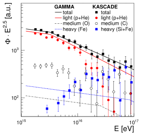
(a) QGSJet01

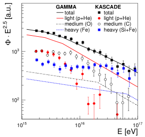
(b) Sibyll2.1

Figure 5: Unfolded fluxes from GAMMA [64] and KASCADE [65] using two different interaction models. The spectra of elemental groups have been adjusted by a common factor (within 35%) to match the all-particle spectra of the two experiments. KASCADE points were slightly displaced in energy for better visibility.

3.1.1 $N_{e}$-$N_{\mu}$ Method

Measuring electron and muon numbers (and their fluctuations) has become the first and most commonly employed technique applied to infer the cosmic ray composition from EAS data. The basic principles of this approach can be understood very intuitively, since the sum of electron and muon numbers measured at ground relates to the primary energy, while the ratio of the muon to electron number relates to the primary mass for reasons described in the previous section. These general features can also be observed in Fig. 3. Fukui et al. [66] and Khristiansen et al. [67] were the first to study the muon number fluctuations in the knee region and they were also the first concluding an enrichment by heavy nuclei above the knee energy [68]. Similar conclusions were drawn in [69] based on a larger data set.

In the most classical approach, electron-muon discrimination is achieved by employing a combination of unshielded and shielded scintillation detectors at ground level. Recent examples include AGASA [70], CASA-MIA [71], EAS-TOP [72], GRAPES [73], KASCADE [74], KASCADE-Grande [75], Maket-ANI [76], GAMMA [64], and Yakutsk [77]. The Pierre Auger Observatory [78] operates water Cherenkov detectors of 1.2 m depth which also enables limited muon identification. The electromagnetic particles (electrons, positrons, and photons) are more numerous than the muons but their mean energy at detector level is only some 10 MeV while that of the muons is about 1 GeV. The former thus produce a large number of relatively small Cherenkov pulses whereas muons produce a small number of large pulses. This type of discrimination technique was pioneered at the Haverah Park detector [79]. Since FADC readout was not available at that time, signal traces of the detectors were photographically recorded from oscilloscopes. IceTop at the South Pole [80] uses tanks of frozen ice instead of water for obvious reasons. Sensitivity to the primary composition is achieved by measuring the dominant electromagnetic component at ground level in IceTop in coincidence with high energy muon bundles in IceCube (muon threshold about 500 GeV), originating from the first interactions in the atmosphere. Similar combinations of surface and underground detectors have been used e.g. by EAS-TOP and MACRO at the Gran Sasso [81] and at the Baksan underground laboratory [82]. Such methods are potentially very attractive for composition studies, as the TeV energy muons measured deep underground probe the energy per nucleon while the surface array probes the energy per particle of the cosmic ray primary. The disadvantage is the reduced statistical accuracy of the muon measurements and the limited solid angle available for coincident cosmic ray observations. Finally, Tibet-AS$\gamma$ [83] complemented their air shower array with emulsion chambers and so-called burst detectors, and Telescope Array (TA) [84] employ solely unshielded scintillation detectors and thus do not discriminate muons from electrons at detector level. Composition studies in these cases rely on additional measurements discussed below.

The importance and proper treatment of air shower fluctuations in any analysis of the nuclear mass composition has already been emphasized. It is important to realize that electron and muon numbers do not fluctuate independently on event-by-event basis, but are mutually correlated (cf. Fig. 3). All these effects can be properly accounted for by a two-dimensional unfolding technique, first utilized by the KASCADE-Collaboration [65, 85]. This approach yields a set of energy spectra of primary mass groups, such that their resulting simulated double differential electron and muon number distribution, $\mathrm{d}^{2}N/\mathrm{d}N_{e}\mathrm{d}N_{\mu}$, resembles the observed one. The only input required for solving the underlying mathematical equations are the so-called kernel functions describing the transformation $(E,A)\to(N_{\mu}^{\rm obs},N_{e}^{\rm obs})$ including their shower-by-shower fluctuations. These functions need to be generated from air shower simulations (including detector response functions) and thus will depend on the chosen hadronic interaction model employed in the EAS simulations. The level of systematic uncertainties imposed by the interaction models can be studied by constructing kernel functions using different hadronic interaction models and comparing the corresponding unfolded results (cf. Fig. 5). Moreover, the observed two-dimensional $(N_{\mu}^{\rm obs},N_{e}^{\rm obs})$ distribution can be directly compared to the forward folded distribution when using the unfolding results as input. Based on such kind of systematic studies the KASCADE Collaboration concluded that neither QGSJet-01 nor Sibyll2.1 is able to describe the full range of energies consistently. Specifically, a muon deficit (or electron excess) has been found for Sibyll2.1 simulations when compared to data [65]. Expressed in terms of the mean logarithmic mass (see below) the two models differ systematically by about half a unit but yield the same basic result of a light (He dominated) composition at the knee with a change towards a heavy composition at higher energies. Moreover, the data are consistent with the assumption of a rigidity dependent change of the knee energy. Similar conclusions about an increasing mass across the knee have been drawn e.g. in [86, 87, 81]. More recently, the GAMMA Collaboration [64] performed a forward folding approach to their electron and muon distributions. In this case, specific spectral shapes are to be defined (here: power-law indices below and above the knee, $E_{\text{k}}/Z$, and the fluxes of four different mass groups). By optimizing the spectral parameters one tries to match the forward folded mean $N_{e}$ vs. $N_{\mu}$ distribution to the measured data. The results of this analysis are included in Fig. 5 and are shown as full and dashed lines. A good description of the all-particle spectrum is again found for a light composition at the knee with an increasing fraction of heavy primaries above. However, differences between forward folding by QGSJet-01 and Sibyll2.1 lead to $\Delta\langle\ln A\rangle\approx 0.7$-$0.8$ with an overall rather light composition (cf. Fig. 14). Data from Tibet AS$\gamma$ [88], on the other hand, seem to suggest an increasing mass composition already below the knee leading to a heavy dominated composition at the knee. This conclusion, however, is based on a number of assumptions and a rather limited statistics of events. Since the set-up and event selection used in Ref. [88] was essentially blind to heavy primaries, the heavy component has been deduced in Ref. [88, 89] rather indirectly by subtracting the flux of the light component (p+He) from the all-particle spectrum measured by Tibet-III [90].

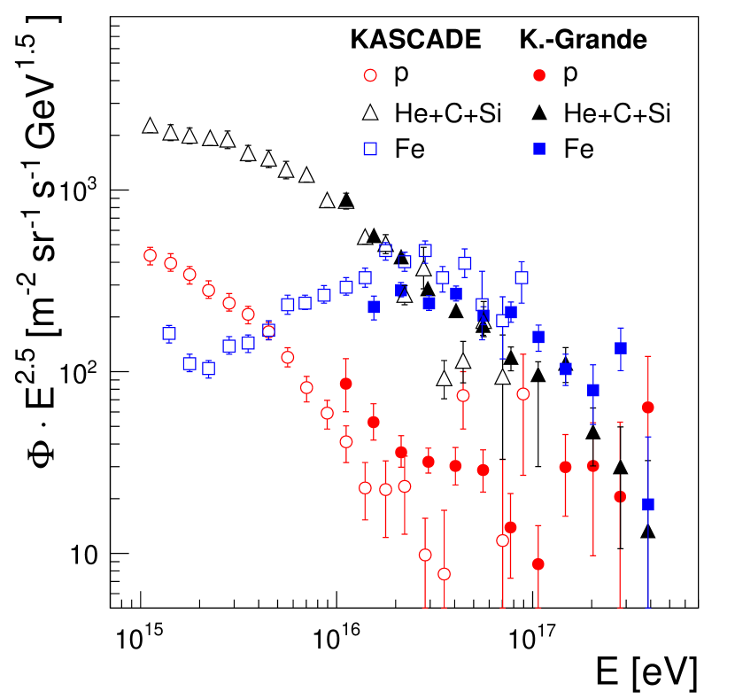
Figure 6: Unfolded fluxes from KASCADE and KASCADE-Grande (open and full symbols, respectively) based on the QGSJet-II-02 interaction model (data are from [91, 92].

Only very recently, data from the KASCADE-Grande experiment reached sufficient statistics allowing the unfolding analyses to be extended to energies nearing $10^{18}$ eV (cf. Fig. 6). Because of poorer detector resolution in KASCADE-Grande, the analysis has been limited to only three mass groups. However, the preliminary unfolding results [92] confirm earlier findings of KASCADE and indicate a very heavy composition at about $10^{17}$ eV . Similar conclusions about the mass composition using electron-poor and electron-rich showers have been drawn in [93] with a knee-like structure observed at $8\times 10^{16}$ eV that could be identified with the heavy component of primary cosmic rays.

3.1.2 Steepness of Lateral Distribution Function

The determination of the lateral density distribution of particles in EAS is the most fundamental task of a particle detector, because the total number of charged particles, electrons, or muons is obtained by fitting the radial fall-off of the measured particle densities to proper analytical functions and performing the radial integration. The energy and mass of the primary particle can then be deduced from the electron and muon numbers, as described in the previous section. Historically, choices of parameterizations of both electron and muon lateral distributions were influenced very much by the seminal review of Greisen [94] in which the analytical calculations performed by Kamata and Nishimura [95] for electromagnetic showers were generalized to the Nishimura-Kamata-Greisen (NKG) function:

$$\rho_{\rm NKG}(r,s,N_{e}) = \frac{N_{e}}{r_{M}^{2}}\;\;\frac{\Gamma(4.5-s)}{2\pi\Gamma(s)\Gamma(4.5-2s)}$$ (26)

$$\times\;\Bigg{(}\frac{r}{r_{M}}\Bigg{)}^{s-2}\Bigg{(}1+\frac{r}{r_{M}}\Bigg{)}^{s-4.5}$$

with the shower age $0.5<s<1.5$, the Molière radius $r_{M}$, and the electron shower size $N_{e}$. A large variety of Lateral Distribution Functions (LDFs) is found in the literature (named Greisen, Greisen-Linsley, etc.), often being specific modifications of the NKG-function aiming at providing an optimum description for either electrons or muons, or both, or are simple power-laws being optimized to describing densities measured by scintillators or water Cherenkov detectors, etc. [96, 97, 98].

Besides being a tool to reconstruct shower sizes, the actual shape of the LDF also contains information about the underlying particle physics in the EAS and, thereby, also about the mass of the primary particle. Generally, showers initiated by heavy primaries and reaching their maximum at high altitudes will exhibit a flatter LDF than those initiated by light primaries and developing deeper into the atmosphere. This feature is observed both for electrons and muons and the steepness of the LDF can be extracted for samples of EAS (properly selected by shower size and zenith angle) [99] or, if sampling statistics does allow, also on event by event basis [97]. A reanalysis of data from Volcano Ranch [100] was performed in Ref. [101] and yielded an iron fraction of about 75% at $E\simeq 10^{18}$ eV, if the QGSJet-01 model was adopted. The sensitivity of the LDF to the primary mass, however, is weaker as compared to the $N_{e}$-$N_{\mu}$ method or those techniques discussed below.

3.1.3 Muon Tracking and Timing

Interest in reconstructing the the mean heights of production of muons in EAS to learn about the longitudinal shower development date back to the 60ies of the last century [102]. However, at that time neither the angular resolution of EAS arrays nor the accuracy of shower simulations were appropriate to the use such measurements for investigating the mass composition of primary cosmic rays. The technique was revived in the 90ies with the Cosmic Ray Tracking (CRT) detectors at HEGRA (aiming at tracking of electrons and muons) [103], the Muon Tracking Detector at KASCADE [104] or at GRAPES [105]. In these detectors the orientation of the muon track is measured with respect to the shower axis and the muon production height is then reconstructed by means of triangulation. For such detectors one needs to find a compromise between a sufficiently long base-line at the ground (i.e. distance between shower core and tracking detector) and a sufficiently large area for the tracking detectors. Increasing the average distance improves the accuracy of the triangulation but shifts the tracking detector in regions of smaller muon densities. A typical compromise at energies around and above the knee is about 100 m baseline or more and at least 100 m² muon tracking area. Based on such measurements, no or only a small rise of the mean mass above the knee was concluded from CRT at HEGRA [106]. However, data were binned as a function of the electron shower size which imposes a strong bias towards electron rich showers, i.e. to light primaries. Measurements of the muon production height with KASCADE-Grande [107] are compatible with a clear transition from light to heavy cosmic ray primary particles with increasing shower energy across the knee.

An attractive alternative to infer the mean muon production depth in EAS was suggested in [108, 109]. Instead of performing a geometrical triangulation by complex and expensive tracking detectors, one measures the time delay of muons in each detector station at ground level with respect to the shower front. Since muons are in general produced close to the shower axis, those muons produced at high altitude can reach a detector station at some distance to the shower core at a shorter average path length as compared to muons produced deep in the atmosphere. Therefore, the relative time delay to the shower front plane is a direct measure of the mean Muon Production Depth (MPD) in the atmosphere. Similarly to the aforementioned muon tracking detectors, the resolution of measurements of the MPD improves both with increasing muon numbers observed in a detector station and with increasing distance of the station to the shower core. However, distortions become large close to the shower core because of limited FADC sampling times and electron contamination. Thus, a proper minimum distance to the shower core needs to be maintained.

A first application of this novel method to real data has been presented by the Pierre Auger Collaboration only very recently [110]. From the MPD distribution measured in each event, the quantity $X_{\mu}^{max}$ can be extracted by fitting a Gaisser-Hillas function [111] to this distribution, where $X_{\mu}^{max}$ can be interpreted as the point where the production of muons reaches the maximum along the cascade development. The resolution in individual events ranges from about 120 g/cm² at the lower energies to less than 50 g/cm² at the highest energy and the systematic uncertainties on $\langle X_{\mu}^{max}\rangle$ were reported 11 g/cm². Within these uncertainties, a mixed composition with a mild change to a heavier composition is reported in [110] for energies above $2\cdot 10^{19}$ (cf. Fig. 14).

3.1.4 Rise-Time

Further information about the primary mass of UHECR is encoded in the time profile of shower particles. This was first noted by Bassi et al. [112] and was used in the context of primary composition at Haverah Park [113, 114, 115]. An advantage of this technique is that it does not require electron-muon discrimination at the detector level, but makes use of the fact that muons are mostly detected near the shower front and that electrons are subject to stronger attenuation in the atmosphere than muons. Full exploitation of this technique, however, requires state-of-the-art FADC read-out electronics. Moreover, it has been noted that the signals from water Cherenkov detectors located upstream of an inclined shower exhibit faster rise-times than those located downstream. This is called the ‘rise-time asymmetry’ [116]. As rise-time we shall understand here the time it takes for the integral signal to increase from 10 to 50% of its full value.

For simple geometrical reasons, no rise-time asymmetry is expected for vertical showers. For very inclined showers one again finds only very small rise-time asymmetries between inner and outer detectors. This can be understood because of the absence of the electromagnetic component and dominance of the high energy muon component in inclined showers, the latter being basically free of asymmetries. The zenith angle at which the rise-time asymmetry becomes maximum, $\theta_{max}$, was demonstrated to be correlated with the shower development [116] and thereby to the average mass of the primary particles. Like the $N_{e}$-$N_{\mu}$ unfolding, this method cannot be applied on an event-by-event basis, which however is no major limitation. A first application to data was presented in Ref. [117] indicating a transition from a light to heavy composition in the energy range $3\times 10^{18}$ to $4\times 10^{19}$ eV (cf. Fig. 14).

3.2 Non-imaging Cherenkov Detectors

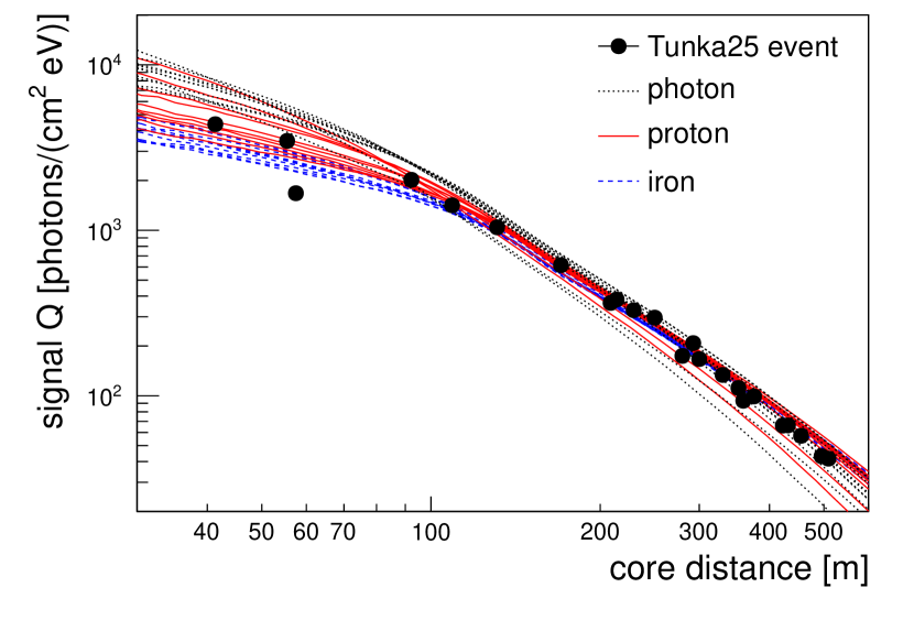
Figure 7: Example of a lateral Cherenkov light distribution as measured with non-imaging Cherenkov detectors. Data points are taken from [118] ($E=0.12$ EeV) and compared to ten simulated [33] air showers for three different primary particle types using the hadronic interaction model QGSJetII [37].

If atmospheric conditions permit, particle measurements at ground are often complemented by observations of Cherenkov or fluorescence light from EAS.

Cherenkov light emitted by extensive air showers in the atmosphere has been known for many years to contain information on shower development [119]. Non-imaging observations by operating PMTs with large Winston cones looking upwards into the night-sky are perhaps the simplest and most straightforward technique of EAS observations. The basic principles have been worked out in [120, 121] and the method was first successfully applied at energies around the knee by the AIROBICC detectors installed at the HEGRA array [122] and by CASA-BLANCA [123] in Utah. More recent measurements at the Tunka [118, 124] and Yakutsk [125] arrays have extended these measurements up to ultra-high energies.

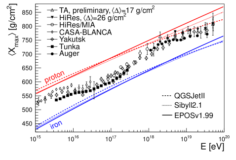
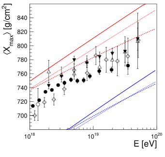
Figure 8: Measurements of $\langle X_{\mathrm{max}}\rangle$ with non-imaging Cherenkov detectors (Tunka [118, 126], Yakutsk [127, 128], CASA-BLANCA [123]) and fluorescence detectors (HiRes/MIA [129], HiRes [130], Auger [131] and TA [132]) compared to air shower simulations [133] using hadronic interaction models [36, 38, 37]. HiRes and TA data have been corrected for detector effects as indicated by the $\langle\Delta\rangle$ values (see text). The right panel shows a zoom to the ultra-high energy region.

The lateral distribution of Cherenkov light at ground is the result of a convolution of the longitudinal profile of charged particles in the shower with the energy threshold for Cherenkov emission and the Cherenkov emission angle which both depend on the air density and thus height. Moreover, the angular distribution of electrons in a shower due to multiple scattering contributes to the lateral extend of Cherenkov light at ground. Because the electron energy distribution (and thus the number of electrons above Cherenkov threshold) as well as their angular distribution are universal in shower age [134, 135, 136, 137], the non-imaging Cherenkov technique provides a model independent method to measure both, the calorimetric energy and shower maximum of air showers.

A characteristic feature of the lateral light distribution at ground is a prominent shoulder at around 120 m from the shower core (cf. Fig. 7) which is due to the strongly forward beamed emission of the Cherenkov light ($\theta_{\text{Ch}}^{\text{\,air}}\approx 1.4^{\circ}$) from near the shower maximum in the atmosphere. The slope of the lateral distribution measured within this 120 m is found to depend on the height of the shower maximum and hence on the mass of the primary cosmic ray nucleus. The overall Cherenkov intensity at distances beyond the shoulder, on the other hand, is closely related to the calorimetric energy.

The $\langle X_{\mathrm{max}}\rangle$ measurements from BLANCA [123], Tunka [118, 126] and Yakutsk [125] are shown in Fig. 8. At low energies ($E<10^{16}$ eV) the three measurements disagree by up to 40 g/cm², but all three detectors observed small elongation rates above $5\times 10^{15}$ eV, indicating a change towards a heavier composition. At around $10^{17}$ eV the absolute values of $\langle X_{\mathrm{max}}\rangle$ from Tunka and Yakutsk are approaching the simulation results for heavy primaries and beyond that energy the average shower maximum increases again towards the air shower predictions for light primaries. At even higher energies, only the Yakutsk array measured ${\langle X_{\mathrm{max}}\rangle}$ with Cherenkov detectors and we will discuss this range in the next section together with the data from fluorescence telescopes.

3.3 Fluorescence Telescopes

After the first prototyping and detection of fluorescence light from air showers [138, 139, 140], the Fly’s Eye detector [141] and its successor HiRes [142] established the measurement of the longitudinal development of air showers using fluorescence telescopes and studied the evolution of the shower maximum with energy [143, 144]. Currently, two observatories are in operation that use the fluorescence technique for the determination of the energy scale and for composition studies: The Pierre Auger Observatory in the Southern hemisphere [145] and the Telescope Array (TA) in the Northern hemisphere [84].

The measurement of the longitudinal air shower development with fluorescence telescopes relies on the fact that the charged secondaries of an air shower excite the nitrogen molecules in the atmosphere that in turn emit fluorescence light. Since the light yields [146] are proportional to the energy deposited in the atmosphere, this observation allows to reconstruct the longitudinal development of the air shower as a function of slant depth.

A typical example of a reconstructed energy deposit profile of an ultra-high energy air shower is shown in Fig. 9. For this particular shower, the full profile was observed and the total calorimetric energy could be obtained by simply adding up the data points. In general, however, only part of the profile can be detected, because the shower either reaches ground or its rising edge is obscured by the upper field of view boundary of telescope. Therefore, the profile is usually fitted with an appropriate trial function [147] that allows the extrapolation of the shower outside of the field of view and to below ground level. Popular choices for fitting longitudinal profiles are the Gaisser-Hillas function [111] (used e.g. by Auger [148]) or a Gaussian in shower age [149] as it was used for the final HiRes analyses. The calorimetric energy of the shower is then given by the integral of the fitted energy deposit profile.

In addition to the calorimetric energy, the measurement of the longitudinal energy deposit profile provides a direct observation of the shower maximum. As can be seen in Fig. 9, where simulated longitudinal shower profiles are superimposed on the measured profile, even on a shower-by-shower basis a rough distinction between heavy and light primaries is possible by comparing the position of ${X_{\mathrm{max}}}$. In principle, the full distribution of shower maxima for showers with similar energy contains the maximum information about composition that can be obtained from fluorescence detectors. Given enough statistics and an exact knowledge of the expected distributions for different primaries, it should be possible to extract composition groups (see e.g. [150]) similar to what is done for surface detectors. In the following, however, we will concentrate on the first two moments of the ${X_{\mathrm{max}}}$-distribution, $\langle X_{\mathrm{max}}\rangle$ and $\sigma(X_{\mathrm{max}})$.

For the determination of the average shower maximum, experiments bin the recorded events in energy and calculate the mean of the measured shower maxima. For this averaging not all events are used, but only those that fulfill certain quality requirements that vary from experiment to experiment, but all analyses accept only profiles for which the shower maximum had been observed within the field of view of the experiment. Without this condition, one would rely only on the rising or falling edge of the profile to determine its maximum, which was found to be to unreliable to obtain the precise location of the shower maximum. The field of view of fluorescence telescopes is typically limited to 1-30 degrees in elevation. Therefore some slant depths can only be detected with smaller efficiencies than others, resulting in a distortion of the measured ${X_{\mathrm{max}}}$-distribution due to undersampling in the tails of the distribution [151, 152]. For instance, a detector located at a height corresponding to 800 g/cm² vertical depth cannot detect shower maxima deeper than 800, 924 and 1600 g/cm² for showers with zenith angles of 0, 30 and 60 degrees respectively. On top of this acceptance bias an additional reconstruction bias may be present that can further distort the measured $\langle X_{\mathrm{max}}\rangle$-values.

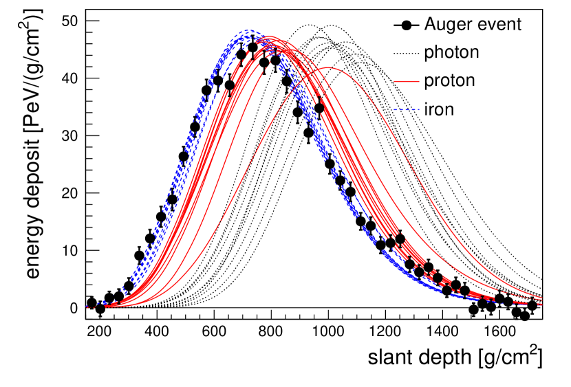
Figure 9: Example of a longitudinal air shower development as measured with fluorescence telescopes. Data points are taken from [145] ($E=(30\pm 2)$ EeV) and compared to ten simulated [133] air showers for three different primary particle types using the hadronic interaction model Epos1.99 [36].

There are two ways to deal with such biases: If one is only interested in comparing the data to air shower simulations for different primary particles, then the biased data can be simply compared to air shower predictions that include the experimental distortions. For this purpose the full measurement process has to be simulated including the attenuation in the atmosphere, detector response and reconstruction to obtain a prediction of the observed average shower maximum, ${\langle X_{\mathrm{max}}\rangle}_{\mathrm{obs}}$. Another possibility is to restrict the data sample to shower geometries for which the acceptance bias is small (e.g. by discarding vertical showers) and to correct the remaining reconstruction effects to obtain an unbiased measurement of $\langle X_{\mathrm{max}}\rangle$ in the atmosphere.

Whereas the former approach maximizes the data statistics, the latter allows the direct comparison of published data to air shower simulations even for models that were not developed at the time of publication. Moreover, only measurements that are independent of the detector-specific distortions due to acceptance and reconstruction can be compared directly.

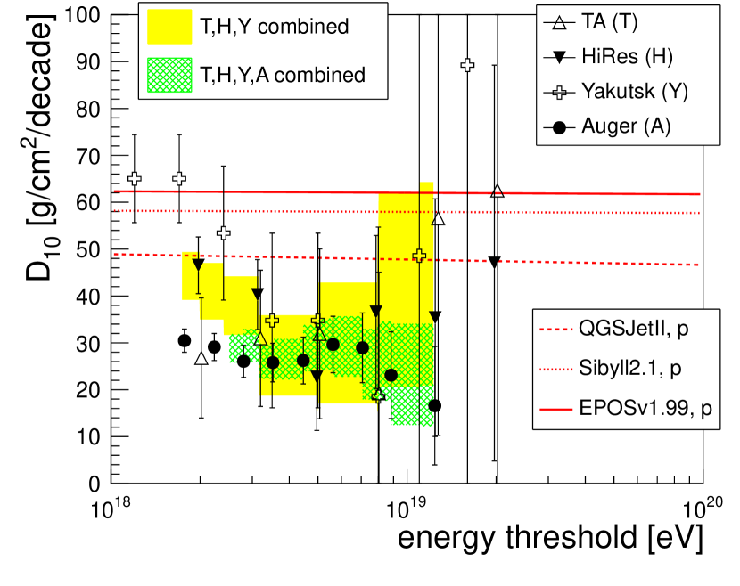
Figure 10: Elongation rates obtained by a linear fit in $\lg E$ to the $X_{\mathrm{max}}$ data of HiRes, Yakutsk, TA and Auger above different energy thresholds. Only fit results with $\chi^{2}/\mathrm{Ndf}<2$ are shown. The yellow, solid band is the average obtained for HiRes, Yakutsk and TA , the green hatched band indicates the average for all four experiments.

The HiRes and TA collaborations follow the strategy to publish ${\langle X_{\mathrm{max}}\rangle}_{\mathrm{obs}}$ [130, 132] and to compare it to the detector-folded air shower simulations. In the HiRes analysis the cuts were optimized to assure an $X_{\mathrm{max}}$-bias that is constant with energy, but different for different primaries and hadronic interaction models. The preliminary TA analysis uses only minimal cuts resulting in energy dependent detection biases. The Auger collaboration quotes average shower maxima that are without detector distortions within the quoted systematic uncertainties [153] due to the use of fiducial volume cuts. Yakutsk derives $X_{\mathrm{max}}$ indirectly using a relation between the slope of the Cherenkov-LDF and height of the shower maximum (cf. Sec. 3.2). This relation is derived from air shower simulations and is universal with respect to the primary particle and hadronic interaction models [154]. We will therefore assume in the following, that the the Yakutsk measurement is bias-free and that it can be compared to air shower simulations directly.

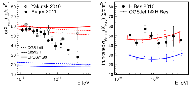
Figure 11: Left: Shower-to-shower fluctuations of ${X_{\mathrm{max}}}$ in the atmosphere as measured by Yakutsk [127] and Auger [131] compared to air shower simulations [133]. Right: Width of a Gaussian fit to the truncated ${X_{\mathrm{max}}}$-distributions as measured by HiRes [130] compared to air shower simulations including detector effects.

To allow a comparison of the results of these experiments and moreover to calculate $\langle\ln A\rangle$ using the Epos model (cf. Sec. 3.4) which was not used in some of the original publications, we correct the ${\langle X_{\mathrm{max}}\rangle}_{\mathrm{obs}}$-values of HiRes and TA by shifting them by an amount $\Delta$ which we infer from the difference of the published ${\langle X_{\mathrm{max}}\rangle}_{\mathrm{obs}}$-values for proton, QGSJetII to the simulated values that are obtained without detector distortions:

$${\langle X_{\mathrm{max}}\rangle}_{\mathrm{corr}}=\langle X_{\mathrm{max}}\rangle_{\mathrm{obs}}+\Delta$$ (27)

where

$$\Delta=\left\langle X_{\mathrm{max}}(\textsc{QGSJetII},\mathrm{p})\right\rangle-\left\langle X_{\mathrm{max}}(\textsc{QGSJetII},\mathrm{p})\right\rangle_{\mathrm{obs}}.$$ (28)

The obtained $\Delta$-values are approximately constant with energy for HiRes with $\langle\Delta\rangle=26$ g/cm². $\Delta$ decreases with energy for TA from $\Delta=24$ g/cm² at $10^{18.3}$ eV to $\Delta=9$ g/cm² at $10^{19.7}$ eV . Although these values correspond to up to 25% of the predicted proton/iron difference, the correction procedure seems justified, because both experiments measured a ${\langle X_{\mathrm{max}}\rangle}_{\mathrm{obs}}$ that is very close to the detector-distorted QGSJetII/proton predictions and the $\Delta$-correction preserves the residuals wrt. this prediction for ${\langle X_{\mathrm{max}}\rangle}_{\mathrm{corr}}$.

The $\langle X_{\mathrm{max}}\rangle$-values measurements from fluorescence detectors are shown in Fig. 8. At around the region of the ankle of the cosmic ray spectrum the measurements are compatible within their quoted systematic uncertainties ($\sim$10 g/cm²) and the ${\langle X_{\mathrm{max}}\rangle}$ is close to the prediction for air showers initiated by a predominantly light composition. Below this energy, the few data points from Auger as well as the HiRes/MIA data confirm the trend observed by the non-imaging Cherenkov detectors, namely a large elongation rate indicative of a transition from a heavy to a lighter composition. A complete coverage of the transition region down to $10^{17}$ eV with new fluorescence detector measurements is expected in the near future with the High Elevation Auger Telescopes (HEAT, operating since 2009) [155] and the Telescope Array Low Energy Extension (TALE, under construction) [156].

At ultra-high energies, the experimental situation can be quantified by fitting the data with a linear function in the logarithm of energy. The resulting elongation rates are summarized in Fig. 10. As can be seen, the elongation rates of the four experiments agree within uncertainties above a few EeV, though the statistical precision deteriorates quickly with increasing energy. Numerical values for fits above $10^{18.6}$ eV are given Tab. 1. Auger, which has collected by far the largest statistics of the four experiments, observes a small elongation rate of $D_{10}=26\pm 5$ (g/cm²)/decade, which could indicate a gradual increase of the average mass of cosmic rays at ultra-high energies if the elongation rate for a constant composition is indeed 50 to 60 (g/cm²)/decade as predicted by the models. This small value of $D_{10}$ is confirmed by HiRes, TA, and Yakutsk, for which the weighted average of elongation rates from Tab. 1 is 27$\pm$9 (g/cm²)/decade.

	$X_{19}$	$D_{10}$	$\chi^{2}$/Ndf
	[$\mathrm{g/cm^{2}}$]	[(g/cm2)/decade]
HiRes	782$\pm$3	23$\pm$11	1.7/4
Yakutsk	773$\pm$5	35$\pm$19	1.9/5
Auger	758$\pm$1	26$\pm$50	1.9/5
TA	774$\pm$5	32$\pm$18	1.4/4

Table 1: Results of a fit with ${\langle X_{\mathrm{max}}\rangle}=X_{19}+D_{10}(\lg(E/\text{eV})-19)$ to ${\langle X_{\mathrm{max}}\rangle}$-data above $10^{18.6}$ eV .

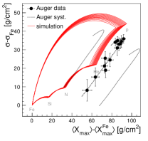
(a) QGSJet01

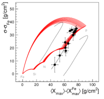
(b) QGSJetII

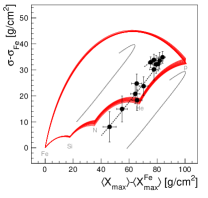
(c) Sibyll2.1

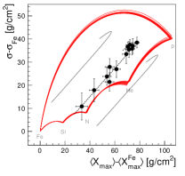
(d) Epos1.99

Figure 12: Comparison of Auger measurements [131] of the average shower depth and its fluctuations with air shower simulations. The energy of the data points increases from top to bottom, as indicated by the dashed line.

The absolute depths at $10^{19}$ eV are, however, in poor agreement among the four experiments and the differences of up to 24 g/cm² between the Auger and HiRes results are larger than expected for individual systematic uncertainties at the 10 g/cm² level. It is worthwhile noting that without the $\Delta$ correction, the three fluorescence detectors agree almost perfectly at ultra-high energies. This might be a mere coincidence or a hint that either HiRes and TA overestimate their bias or that the assumption of $\Delta\approx 0$ does not hold for Auger.

As explained in Sec. 2.1, the fluctuations of the shower maximum provide another composition sensitive observable. The measurements of $\sigma(X_{\mathrm{max}})$ from Auger and Yakutsk are shown in the left panel of Fig. 11. Both data sets were corrected for the detector resolution and can thus be directly compared to air shower simulations. The Auger data exhibits a significant narrowing of the $X_{\mathrm{max}}$ distributions with energy starting at about the energy of the ankle. The low energy width is compatible with a light or mixed composition, but the small $\sigma(X_{\mathrm{max}})$ at high energies points to the presence of a significant fraction of CNO or heavier nuclei with little admixture of light nuclei (cf. Eq. (12)). The data of the Yakutsk array are compatible with a light composition at all energies. Below $10^{19.3}$ eV there is a good agreement with the Auger results, but their last data point is in contradiction with the small width quoted by Auger.

The fluctuation measurements of HiRes are shown in the right panel of Fig. 11. Instead of $\sigma(X_{\mathrm{max}})$, HiRes published the width of a Gaussian fit to the $X_{\mathrm{max}}$-distributions that were truncated at $\pm 2{\sigma(X_{\mathrm{max}})}$ without correction for detector resolution. This variable can then be compared to air shower simulations including detector effects. As can be seen, HiRes finds a large width at low energy that is, similar to Auger and Yakutsk, compatible with a light or mixed composition. Above $10^{19}$ eV the width remains compatible with proton simulations, albeit with large statistical uncertainties that could also accommodate a narrower width.

The compatibility of the $\langle X_{\mathrm{max}}\rangle$ and $\sigma(X_{\mathrm{max}})$ measurements with air shower simulations can be studied within the $\sigma({X_{\mathrm{max}}})$-${\langle X_{\mathrm{max}}\rangle}$ plane introduced in Sec. 2.1. The Yakutsk data would cluster at around the simulated proton values in this plane and the HiRes data cannot be analyzed in this way without a full detector simulation. Therefore only the Auger data are shown in Fig. 12.

If hadronic interactions at ultra-high energies are modeled correctly and if the cosmic ray composition is any mixture of elements between proton and iron, then the data points must lie within the contours shown in Fig. 12. As can be seen, this is not the case for the outdated QGSJet01 model. For both, QGSJetII and Sibyll2.1, the Auger data are barely at the edge of the contour, which would imply a somewhat unnatural transition from a proton- to helium- to nitrogen-dominated composition. Using Epos1.99, the corresponding composition would be mixed at low energies and very nitrogen-rich at high energies. Whereas these considerations clearly demonstrate the power of a combined observation of $\langle X_{\mathrm{max}}\rangle$ and $\sigma(X_{\mathrm{max}})$, the current systematic uncertainties of the Auger measurements do not allow for a stringent test of the models: If the Auger data are shifted simultaneously by $\pm\mathrm{syst}(E)$, $\mp\mathrm{sys}({\langle X_{\mathrm{max}}\rangle})$ and $\pm\mathrm{syst}({\sigma(X_{\mathrm{max}})})$ as in [157] (indicated by lines in Fig. 12), then even for QGSJet01 a marginal compatibility remains.

3.4 Average Logarithmic Mass

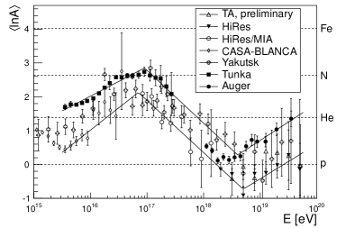
(a) QGSJet01

(b) QGSJetII

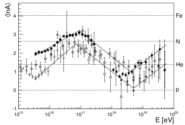
(c) Sibyll2.1

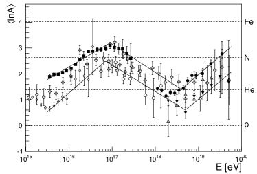
(d) Epos1.99

Figure 13: Average logarithmic mass of cosmic ray as a function of energy derived from ${X_{\mathrm{max}}}$ measurements with optical detectors for different hadronic interaction models. Lines are estimates on the experimental systematics, i.e. upper and lower boundaries of the data presented.

As it should have become clear in the previous sections, the measurement of the mass composition of cosmic rays from air shower data is a challenging task. There are still considerable systematic differences between the various air shower measurements that need to be resolved. A further obstacle arises from the large shower-by-shower fluctuations of air shower observables which are found to fluctuate at a level which, for light primaries, may become comparable to the mean separation of proton and iron primaries. Moreover, and maybe most importantly, the interpretation of these measurements in terms of the chemical composition of cosmic rays relies on the validity of models of hadronic interactions at ultra-high energies.

The best discrimination power in terms of models for the origin of ultra high energy cosmic rays is of course given by a determination of the energy dependence of different groups of primary elements. But as could be seen in e.g. Fig. 5, even when different experiments use the same hadronic interaction model to interpret their data, there are large differences in the quoted fluxes of elemental groups and similar discrepancies can be observed when comparing the unfolding results using different interaction models. Part of these difficulties arise due to the large negative correlations between the unfolded elemental fluxes, which are however not quoted by the experiments.

We therefore restrict ourselves to a comparison of the average logarithmic mass of cosmic rays, which we obtain from either

$${\langle\ln A\rangle}=\sum f_{i}\ln A_{i}$$ (29)

for experiments that derived elemental groups of mass $A_{i}$ with flux fractions $f_{i}$ or from

$${\langle\ln A\rangle}=\frac{\langle X_{\mathrm{max}}^{\mathrm{p}}\rangle-\langle X_{\mathrm{max}}^{\mathrm{data}}\rangle}{\langle X_{\mathrm{max}}^{\mathrm{p}}\rangle-\langle X_{\mathrm{max}}^{\mathrm{Fe}}\rangle}\ln 56$$ (30)

in case of experiments that measured $\langle X_{\mathrm{max}}\rangle$. For the latter, model uncertainties can be estimated by using different predictions for $\langle X_{\mathrm{max}}^{\mathrm{Fe}}\rangle$ and $\langle X_{\mathrm{max}}^{p}\rangle$. This comparison is shown in Fig. 13, where we also include the QGSJet01 model for completeness, due to the ubiquity of results from particle detectors that used this superseded model. Obviously, the systematic differences in $\langle X_{\mathrm{max}}\rangle$ discussed in the last section propagate directly to $\langle\ln A\rangle$. To guide the eye and to be able to compare the results from optical detectors with those of particle detectors (see below), the upper and lower $\langle\ln A\rangle$ ranges are sketched in Fig. 13 by solid lines. As can be seen, the experimental systematics in $\langle X_{\mathrm{max}}\rangle$ translates to an uncertainty of about $\sigma({\langle\ln A\rangle})\approx\pm 0.5$. The composition trends that were already visible in Fig. 8 can again be observed in $\langle\ln A\rangle$: All model interpretations suggest a gradual increase of the average logarithmic mass of cosmic rays between $10^{15}$ eV and $10^{17}$ eV followed by a transition towards a lighter composition during the next decade. The heaviest composition with $\langle\ln A\rangle$ $\approx 3.5$ follows from the Tunka data interpreted with QGSJetII at around $10^{17}$ eV . The $\langle\ln A\rangle$ values of HiRes and TA are compatible with a pure proton composition when using one of the two QGSJet-flavors. A trend towards a heavier composition would follow from Auger data for all models and also for HiRes and TA if interpreted using Sibyll or Epos. It is interesting to note that the next version of QGSJetII [158] for which some model parameters were re-tuned to new data from the LHC will have a similar ${\langle X_{\mathrm{max}}\rangle}$ as Sibyll and thus the combination of any of the ${\langle X_{\mathrm{max}}\rangle}$ data with one of the contemporary versions of the three available interaction models will result in a ${\langle\ln A\rangle}$ significantly different from zero at ultra-high energies.

Particle detectors usually do not publish air shower observables but directly the interpretation in terms of elementary fractions, and in that case only the differences between models with which the data were analyzed can be used for a limited estimate of the theoretical uncertainties. Results that were obtained with out-dated interaction models like e.g. the AGASA measurements [159] will be ignored in the following. Since usually only fractions of elemental groups are quoted it is not obvious which value of $\ln A_{i}$ to assign in Eq. (29). To translate the data from Tibet AS$\gamma$ [89] into $\langle\ln A\rangle$, we assume equal fluxes of protons and helium and assign to ‘heavy’ fragments $A=32$. However, we note that the chosen procedure of comparing fluxes from different measurement campaigns with different event selection and energy calibration may introduce additional systematic uncertainties particularly in view of the steep power-law spectra involved, which we can not account for here. For KASCADE-Grande [92], where the intermediate mass group is composed of He, C, and Si, we again assume equal fluxes and take the logarithmic mean of $A\simeq 12$. For data that were analyzed in a simple bimodal proton/iron model like [101, 99] the ${\langle\ln A\rangle}$ calculation is technically easy, but it is difficult to assess the systematic uncertainty arising from this simplified model. Data from EAS-TOP are based on electrons and GeV muons [160] as measured in the calorimeter at the surface as well as on electrons and TeV-muons, the latter measured in MACRO [81]. Of all the experimental particle detector results studied here, only Auger published the measured air shower observables rather than their interpretation. Since the average muon production depth and the rise time asymmetries are well correlated with ${X_{\mathrm{max}}}$ we assume that they also depend linearly on ${\langle\ln A\rangle}$ and can therefore use the air shower simulations folded with the detector response from [117] and [110] to estimate ${\langle\ln A\rangle}$ from the equivalent of Eq. (30) for these variables.

The resulting energy evolution of ${\langle\ln A\rangle}$ as derived from particle detector data is displayed in Fig. 14 for different hadronic interaction models. The upper and lower experimental boundaries from optical detectors are indicated by the superimposed lines. As can be seen, the systematic differences between experimental results at low energies are considerably larger than in the case of optical detectors spanning a range of up to $\Delta{\langle\ln A\rangle}\approx\pm 1$. Nevertheless, all experiments below $10^{17}$ eV report a rise of ${\langle\ln A\rangle}$ with energy that could be reconciled with the ${\langle X_{\mathrm{max}}\rangle}$ results by an appropriate rescaling. In the energy region toward the ankle, surface detector data are sparse. The Haverah Park results tend towards a lighter composition at $10^{18}$ eV , though with large statistical uncertainties. At ultra-high energies only the surface detector data from Auger are available for an interpretation with modern hadronic interaction models. For both simulations, using QGSJetII and Sibyll2.1, these data are compatible with an increase of ${\langle\ln A\rangle}$ above $10^{19}$ eV .

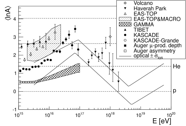
(a) QGSJet01

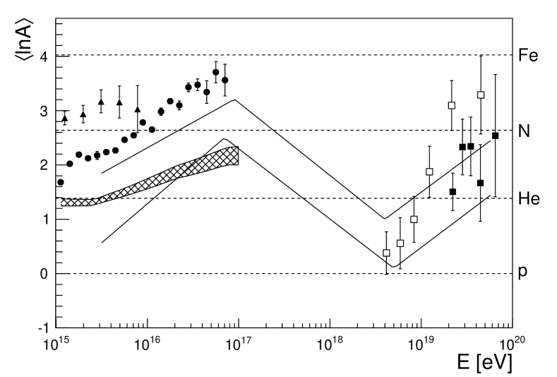
(b) Sibyll2.1

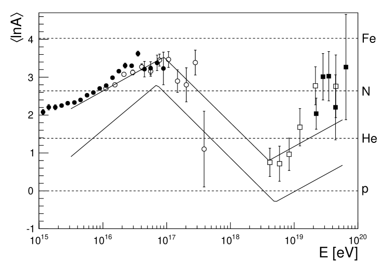
(c) QGSJetII

Figure 14: Average logarithmic mass of cosmic ray as a function of energy derived from particle detector measurements for different hadronic interaction models. Lines are the upper and lower bounds from optical measurements (cf. Fig. 13) for the corresponding model.

4 Search for Neutral Primaries

Measurements of neutral primaries, i.e. neutrons, photons, and neutrinos provide additional crucial information about the acceleration models and sources of cosmic rays as well as on their propagation through the universe. Unlike charged cosmic rays they are not deflected by magnetic fields and could point back to their sources. Specifically, high energy neutrinos pointing back to a source would provide the first unambiguous signal of a high energy cosmic ray accelerator. Moreover, a ‘guaranteed’ flux of high energy photons and neutrinos is provided by the GZK-effect (see Sec. 1). An observation of such cosmogenic neutrinos or photons is considered as a ‘smoking gun’ that would complement the observation of the flux suppression seen in the cosmic ray energy spectrum. Neutrons arise at all energies from charge exchange interactions at the source or in the interstellar medium. However, their lifetime limits their propagation distance to about $10\,\mathrm{kpc}\cdot(E/\!{\mathrm{\ Ee\kern-1.00006ptV}})$.

Separating neutron- from proton-induced showers is not possible. Nevertheless, samples of air showers can be enriched with respect to light primaries and searches for neutron point sources can be performed. Such studies have yielded no detection yet and are reviewed in [21]. Separating photon- or neutrino-induced EAS from nuclei-induced showers is experimentally much easier than distinguishing light from heavy nuclear primaries.

In this chapter we will review recent photon and neutrino searches aimed at highlighting their complementarity to measurements of the nuclear composition.

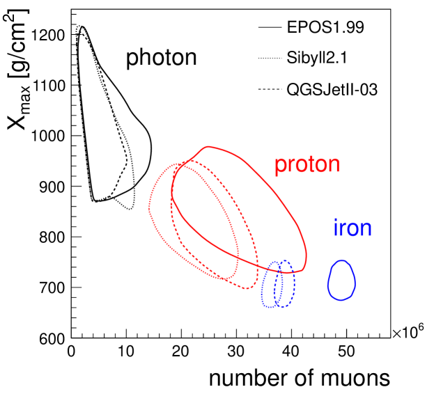
Figure 15: Simulation of hybrid air shower observation: Shower maximum vs. number of muons at ground level (60^∘ shower at 800 g/cm²) for primary energies of $10^{19}$ eV . Contour lines illustrate the regions which include 90% of the showers.

4.1 Photons

Air showers induced by primary photons develop an almost pure electromagnetic cascade and differ from hadron induced ones by their low number of muons and their deep $X_{\mathrm{max}}$. This is illustrated in Fig. 15 for different primaries at $10^{19}$ eV . Since mostly electromagnetic processes are involved in the shower development, the predictions are more reliable and do not suffer from uncertainties in the hadronic interaction models. The Pierre Auger Observatory has the advantage of being a hybrid observatory in which the position of the shower maximum is measured by fluorescence telescopes with simultaneous access to the muon number from the surface detector stations. In case muons cannot be identified, such as in pure scintillator arrays located at the surface, the particle densities at large distances from the shower core combined with measurements of the energy by e.g. fluorescence telescopes can still provide good discrimination power.

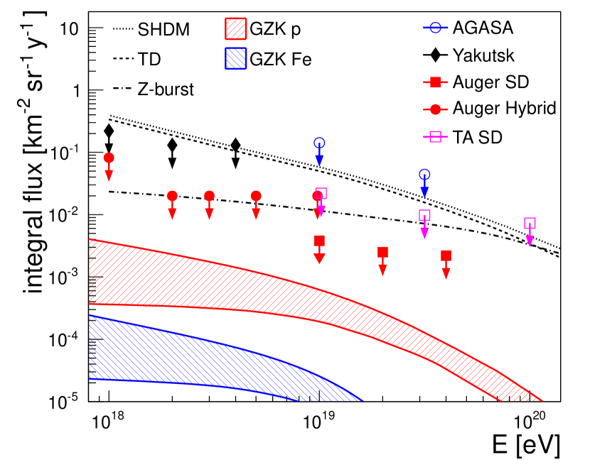
Figure 16: Integral photon flux limits at 95% C.L. from AGASA [161], Yakutsk [162], Auger [163, 164] and TA [165] compared to flux predicitons for GZK-photons [166], top-down scenarios of super-heavy dark matter (SHDM) [167] and topological defect (TD) models, and $Z$-bursts [168].

Early searches for UHE photons, summarized e.g. in Ref. [169], were motivated by particle physics models of UHECR origin. In these so-called top-down models (see e.g. [170] for an early review) the highest energy cosmic rays are decay products of super-heavy relic particles or topological defects (TD) left over from the inflationary epoch and which are locally clustered in the galactic halo as cold dark matter. Their decay yields a relatively high flux of UHE photons and neutrinos reaching up to 90 % of the CR flux. The Z-Burst model [171, 172] involves resonant interactions of very energetic neutrinos with the relic neutrino background. These models are compared to experimental data in Fig. 16. The integral photon flux limits from AGASA [161], Yakutsk [162], and TA [165] are based on muon numbers and curvature of the shower front. The hybrid data of the Pierre Auger Observatory, employing $X_{\mathrm{max}}$ and various SD-observables, provide the best present limits up to $10^{19}$ eV while the Surface Detector data alone extend the best present limits up to $5\times 10^{19}$ eV due to the much higher statistics [163, 164] available in this data set.

The results demonstrate that particle physics motivated top-down models are strongly disfavored giving support to an astrophysical origin of UHECR.

The two bands below the experimental data depict photon fluxes expected from interactions of UHECR with photon background fields, most prominently the Cosmic Microwave Background (CMB) radiation. Both, proton and iron primaries have been considered in these calculations. A power law energy spectrum is assumed with index $\gamma=-2$ and a maximum CR energy at the source of $10^{21}$ eV . The fluxes are normalized to the number of events measured by Auger [173] for energies $E>10^{18.4}$ eV. The upper and lower bounds for each primary result from more or less favorable radio background fields and different cosmological source evolutions [166]. According to these simulations, chances of observing GZK-photons appear well in reach if the source spectrum at the highest energies is dominated by light primaries. Moreover, further improvements, besides increasing statistics of data, may be expected from multivariate analyses of fluorescence and surface detector data. Also, further upward and downwards modifications of the predicted photon flux may result from different energy spectra and/or different maximum energies of the nearby sources [166, 174].

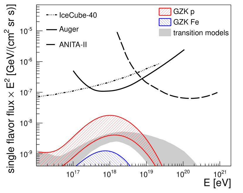
Figure 17: Compilation of 90 %CL single-flavor upper limits for diffuse neutrino fluxes assuming a proportion of flavors of 1:1:1 due to neutrino oscillations. Data are from IceCube [175], Auger [176] and ANITA [177]. The shaded area corresponds to expected GZK neutrino fluxes computed under different assumptions of source evolution scenarios [166] with power-law energy spectra of $\gamma=-2.0$ and $E_{\rm max}^{Z}=Z\cdot 10^{20}$ eV. The grey band depicts different transition models and source evolutions adapted from Ref. [178] (see text for details).

4.2 Neutrinos

Possible neutrino primaries may be the easiest to identify in EAS experiments because of the many orders of magnitude difference between the electroweak and hadronic cross sections. With a neutrino-nucleon cross section of about $\sigma_{\nu N}\simeq 10$ nb at 1 EeV, neutrinos may interact at any point in the atmosphere or even in the rock of the Earth. Thus, showers starting very deep in the atmosphere are likely to be initiated by a primary neutrino. Identification of such showers is easiest in horizontal direction ($\theta>85^{\circ}$) where the atmospheric thickness is effectively 30 times that of the vertical direction. Thus, horizontal showers containing still an appreciable electromagnetic component (so-called ‘young showers’) can only be caused by primary neutrinos. Larger experimental apertures than for near-horizontal showers induced by so-called ‘down-going’ neutrinos are reached for ‘up-going’ tau neutrinos skimming the Earth at zenith angles between $90^{\circ}$ and $96^{\circ}$. After a possible $\nu_{\tau}$-interaction, the produced $\tau$ will be able to escape the Earth and decay in the atmosphere or close to ground producing an upward-going EAS.

Such signatures have been searched for in ground based EAS observatories such as Auger [179] and HiRes [180] reaching highest sensitivities around $10^{18}$ eV , thus matching very well the peak in the differential $E_{\nu}^{2}\text{d}j_{\nu}/\text{d}E_{\nu}$ fluxes of cosmogenic neutrinos. At even higher energies, radio based observations such as ANITA [177] start to take over, while IceCube provides unprecedented sensitivities towards lower energies. The three experimental approaches complement each other very effectively with each of them having improved their sensitivities by orders of magnitudes in the last decade (cf. Fig. 17).

Similarly as for UHE photons, these searches did not detect any neutrino fluxes yet but provided upper limits. Fig. 17 depicts some exemplary reference predictions again for sources emitting proton and iron primaries [166, 178]. Due to their low cross-section, neutrinos — other than photons — suffer only adiabatic energy loss, so that they can arrive at Earth from cosmological distances. As a result, a large level of uncertainty in the flux prediction results from the unknown cosmological evolution of source luminosity, as has been realized already in [181]. The upper dashed bands shown in Fig. 17 are obtained for an FR-II type distribution while the lower one results for a star formation like evolution. As for the photon predictions, power law source distributions with an injection index of $\gamma=-2$ have been assumed as a reference with $E_{\rm max}^{Z}=Z\cdot 10^{20}$ eV. A fit to the Auger CR energy spectrum performed e.g. in [166, 182] yields somewhat steeper source spectra but higher maximum energies of the sources with essentially compensating effects with regard to the neutrino fluxes. The grey band, adapted from Ref. [178], depicts neutrino predictions covering different transition models (dip-model at top and ankle model at bottom) and source evolutions.

Atmospheric neutrinos in the TeV to PeV range are primarily of interest, because they constitute the background in neutrino telescopes such as IceCube [175] or Antares [183]. The cosmic rays producing this ‘calibrated’ beam of neutrinos most dominantly originates from energies above the knee. Thus, an interesting question to ask is the level of uncertainty in the neutrino flux calculations that arises from the poorly known composition (see e.g. [184]). Expressed differently, one may ask whether a comparison of the measured atmospheric neutrino spectra with flux calculations based on cosmic ray energy spectra could provide independent information about the composition at the knee and above. A quantitative study of this question has been presented very recently in Ref. [185]. It used the two different sets of energy spectra shown in Fig. 5 from KASCADE [65] combined with direct measurements of cosmic rays at lower energies as input to a full Monte Carlo simulation. Based on this study, the authors concluded that uncertainties in the all-particle cosmic ray flux appear more important for the neutrino fluxes than the actual uncertainties of the composition arising from the unfolding based on QGSJet versus Sibyll interaction models.

5 Conclusions

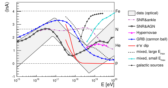
Figure 18: Compilation of $\langle\ln A\rangle$-values from recent astrophysical models compared to the uncertainty range of experimental data (optical detectors, see text). Models include the purely galactic scenario of [9], a mixed extra-galactic composition with a large [11] or small [23] maximum energy of the sources, the ankle and dip model [8], the cannonball model [186], a hypernova model [187], and the SNR-AGN model of [188].

In 1983, Linsley counted the number of contributions submitted to the 18th ICRC that were related to the composition of cosmic rays and concluded [51]

Assuming that people wouldn’t spend effort on this problem unless they believe it can eventually be solved, I think the numbers are encouraging.

Today, almost 30 years later, the quest for the understanding of the primary composition of cosmic rays continues and, although the problem is not fully solved yet, there has been considerable progress in at least our qualitative understanding of the primary cosmic ray composition thanks to the wealth of new data collected by both cosmic ray observatories and particle physics experiments.

At the energies between $10^{15}$ eV and $10^{17}$ eV all experiments observe energy dependent changes in the shower development that are compatible with increasing average mass of cosmic rays. Moreover, unfolded spectra of mass groups in this energy range suggest that the change of composition is attributable to a consecutive cut-off in the flux of the individual mass components starting with protons at a few $10^{15}$ eV up to iron at around $10^{17}$ eV (cf. Figs. 5 and 6). These composition measurements are thus compatible with an interpretation of the knee in the particle flux due to a rigidity dependent leakage of cosmic rays from the galaxy and/or a rigidity dependent maximum energy of galactic sources. At the same time, a particle physics interpretation of the knee is disfavored, since the interaction models used for the interpretation of cosmic ray data were found to bracket particle production measurements from the LHC [62] at 7 TeV center of mass energy, corresponding to a primary cosmic ray energy of $10^{16.4}$ eV .

Towards the energy region of the ankle, air shower measurements indicate a decrease of the average mass of cosmic rays. Both the shower-to-shower fluctuations and the average shower maximum are compatible with a predominantly light composition at a few $10^{18}$ eV . Estimates of the proton-air cross section [189, 190, 191] at this energy agree well with the extrapolations used in hadronic interaction models, therefore also here a drastic change of the interpretation of the measurements in terms of cosmic ray composition due to uncertainties in air shower simulations seems unlikely.

At the highest energies, above $10^{19}$ eV , the experimental uncertainties are still too large to draw firm conclusions from the data. The measurements from Auger of ${\langle X_{\mathrm{max}}\rangle}$, ${\sigma(X_{\mathrm{max}})}$, muon production depth and rise-time asymmetries may be interpreted as a transition to a heavier composition that may be caused by a Peters-cycle in extra-galactic sources similar to what has been observed at around the knee. However, the ${\langle X_{\mathrm{max}}\rangle}$-measurements from HiRes, TA and Yakutsk indicate a systematically lighter composition at these energies but with an elongation rate compatible with Auger (cf. Tab. 1).

These experimental differences together with the uncertainties of hadronic interactions make an astrophysical interpretation of the $\langle\ln A\rangle$ estimates at the highest energies difficult. In Fig. 18 we present a compilation of astrophysical models for the composition of cosmic rays together with the $\langle\ln A\rangle$ inferred from air shower measurements. Here, we show only results from optical measurements, since these are more abundant over the full energy range and — judging from the differences of results from surface detectors at low energies in Fig. 14(a) — are also less affected by experimental systematics. The gray band is the maximum and minimum of the envelopes from Fig. 13, i.e. the upper and lower level of experimental and model differences. The curves represent predictions by recent models about the origin of cosmic rays with a focus on models at ultra-high energies (see [192] and references therein for a comprehensive list of models of cosmic rays around the knee). A fairly good description of $\langle\ln A\rangle$ over the entire energy range is given by the two-component model of [188] in which it is assumed that CRs up to $10^{17}$ eV are produced in galactic supernova remnants while the dominant component at higher energies is of extragalactic origin produced at the shock created by the expanding cocoons around active galactic nuclei. The dashed violet curve shows the classical ankle model and the two red lines the so-called dip-model [8] (actual calculation used are from  [11]). Other than the ankle model, the dip model assumes that the transition from galactic to extragalactic models occurs below the ankle and that the ankle is caused by $e^{+}e^{-}$-interactions of protons in the CMB rather than by the onset of the extragalactic cosmic ray component. To make this Bethe-Heitler process work, the composition above $10^{18}$ eV must be dominated by protons. The blue curve represents the generalized cannonball model [186] in which cosmic rays are described as being ions of the interstellar medium that encountered cannonballs — highly relativistic bipolar jets of plasmoids originating from supernova explosions and GRBs — and were magnetically kicked up to higher energies. In Ref. [187] (shown as the full magenta line with triangles) it has been suggested that hypernova remnants, with a substantial amount of energy in semi-relativistic ejecta, can accelerate intermediate mass or heavy nuclei to ultra-high energies. A heavy composition at the highest energies is obtained in a model where UHECRs were produced by gamma-ray bursts or rare types of supernova explosions that took place in the Milky Way in the past [9]. Finally, the models labels ‘mixed’ with large and small $E_{\rm max}$, are taken from Refs. [11, 23]. Here, a source composition similar to galactic CRs is assumed with the ankle marking again the transition from galactic to extragalactic CRs. In the first realization of the model it is assumed that the maximum energy follows $E_{\rm max}^{\rm high}=Z\cdot 10^{20.5}$ eV with an injection index at the source of $\gamma=-2.0$ [11] whereas in the latter $E_{\rm max}=Z\cdot 4\times 10^{18}$ eV and $\gamma=-1.6$ [23].

While data and models agree reasonably well up to the ankle energy, there is almost the full range of masses covered by models at energies above $10^{19}$ eV . This may be understood from the large uncertainties of experimental data points in this energy range. At present neither a composition dominated by light primaries nor by heavy primaries can safely be ruled out by the data.

As discussed in this paper, a large part of these uncertainties can be attributed to the uncertainties of hadronic interaction models, but also systematic differences between the experimental data itself contribute significantly to the large width of the $\langle\ln A\rangle$-range at the highest energies. Fortunately, hadronic interaction models will improve considerably in the near future due to the new particle production data from LHC. At the same time further improvements of the quality of air shower data are expected because of better instruments and the prospects of a combined analysis of the data of surface and optical detectors with either existing hybrid detectors or enhancements such as e.g. shielded muon detectors in Auger [193].

Additional constraints about the charge of cosmic rays may be acquired from the anisotropy (or lack thereof) of the arrival directions of cosmic rays. The Pierre Auger Collaboration has reported directional correlations of the most energetic particles ($E>5.5\times 10^{19}$ eV) with the positions of nearby AGN [194, 195, 196]. Since the turbulent component of the galactic magnetic field randomizes the arrival directions of particles with small rigidities (i.e. large charge and therefore mass), such a correlation seems to suggest a dominance of light particles at these energies, but it may be still possible that a large scale anisotropy, e.g. from the super-galactic plane, remains anisotropic even after the passage of heavy particles through the turbulent magnetic field [197].

A next generation giant observatory should be able to collect large statistics for both, charged particle astronomy and composition analyses above the GZK threshold. If cosmic rays are extragalactic and their flux at earth is not dominated by very close sources, then the composition analysis at GZK-energies will be facilitated by the suppression of any intermediate nuclei between proton and iron at earth due to the different energy loss lengths of nuclei [11]. In such a simple situation with a ’guaranteed’ composition of protons and iron only it should be possible to simultanously determine the properties of cosmic rays and hadronic interactions at energies above $\sim 6\times$$10^{19}$ eV .

So without any doubt, measurements of the cosmic ray composition up to $10^{20}$ eV remain one of the most important tasks for the future and the key to the understanding of the origin of the most energetic particles in the Universe.

6 Acknowledgement

We would like to thank S.P. Knurenko and V. Prosin for providing data tables and valuable information on the Yakutsk and Tunka data and the Pierre Auger and TA Collaboration for permission to use their data prior to journal publication. Furthermore we would like to express our gratitude to our colleagues in the Pierre Auger and KASCADE-Grande collaborations for many inspiring discussions about the cosmic ray composition and we appreciate the critical reading of the manuscript of this article by R. Clay, C. Dobrigkeit, D. Veberič and the anonymous journal referee.

References

- [1] B. Peters, Nuovo Cimento 22 (1961) 800.
- [2] J. R. Hörandel, Astropart. Phys. 21 (2004) 241.
- [3] D. Allard et al., JCAP 0810 (2008) 033.
- [4] R. Aloisio, V. Berezinsky, A. Gazizov, Astropart. Phys. 34 (2011) 620.
- [5] D. Hooper, A. M. Taylor, Astropart. Phys. 33 (2010) 151.
- [6] K. Greisen, Phys. Rev. Lett. 16 (1966) 748.
- [7] G. Zatsepin, V. Kuzmin, JETP Lett. 4 (1966) 78.
- [8] V. Berezinsky, A. Gazizov, S. Grigorieva, Phys. Rev. D74 (2006) 043005.
- [9] A. Calvez, A. Kusenko, S. Nagataki, Phys. Rev. Lett. 105 (2010) 091101.
- [10] T. Wibig, A. W. Wolfendale, J. Phys. G 31 (2005) 255.
- [11] D. Allard, E. Parizot, A. Olinto, Astropart. Phys. 27 (2007) 61.
- [12] A. Hillas, J. Phys. G 31 (2005) R95.
- [13] R. Aloisio et al., Phys. Rev. D77 (2008) 025007.
- [14] C. De Donato, G. Medina-Tanco, Astropart. Phys. 32 (2009) 253.
- [15] E. Berezhko, Astrophys. J. 698 (2009) L138.
- [16] A. Castellina, F. Donato, Vol. 5 of Planets, Stars and Stellar Systems, Springer, 2012.
- [17] E. Seo, Astropart. Phys. this volume.
- [18] M. Boezio, Astropart. Phys. this volume.
- [19] V. Berezinsky, G. Zatsepin, Phys. Lett. B28 (1969) 423.
- [20] J. Puget, F. Stecker, J. Bredekamp, Astroph. J. 205 (1976) 638.
- [21] P. Sommers, Astropart. Phys. this volume.
- [22] R. Aloisio, V. Berezinsky, Astropart. Phys. this volume.
- [23] D. Allard, Astropart. Phys. this volume.
- [24] M. Nagano, A. A. Watson, Rev. Mod. Phys. 72 (2000) 689.
- [25] J. Blümer, R. Engel, J. R. Hörandel, Prog. Part. Nucl. Phys. 63 (2009) 292.
- [26] K. Kotera, A. Olinto, Annu. Rev. Astron. Astrophys. 49 (2011) 119.
- [27] A. Letessier-Selvon, T. Stanev, Rev. Mod. Phys. 83 (2011) 907.
- [28] J. Engel et al., Phys. Rev. D46 (11) (1992) 5013.
- [29] R. Glauber, G. Matthiae, Nucl. Phys. B21 (1970) 135.
- [30] N. N. Kalmykov, S. S. Ostapchenko, Sov. J. Nucl. Phys. 50 (1989) 315.
- [31] N. Kalmykov, S. Ostapchenko, Phys.Atom.Nucl. 56 (1993) 346.
- [32] G. Schatz et al., J. Phys. G 20 (1994) 1267.
- [33] D. Heck et al., Forschungszentrum Karlsruhe FZKA 6019.
- [34] S. Sciutto AIRES Reference Manual. arXiv:astro-ph/9911331.
- [35] S. Roh et al., AIP Conf. Proc. 1367 (2011) 177.
- [36] T. Pierog, K. Werner, Phys. Rev. Lett. 101 (2008) 171101.
- [37] S. Ostapchenko, Phys. Rev. D83 (2011) 014018.
- [38] E. Ahn et al., Phys. Rev. D80 (2009) 094003.
- [39] J. Knapp et al., Astropart. Phys. 19 (2003) 77.
- [40] J. Carlson, J. Oppenheimer, Physical Review 51 (1937) 220–.
- [41] W. Heitler, Oxford University Press, 1954.
- [42] J. Alvarez-Muniz et al., Phys. Rev. D66 (2002) 033011.
- [43] J. Matthews, Astropart. Phys. 22 (2005) 387.
- [44] J. R. Hörandel, Mod. Phys. Lett. A22 (2007) 1533.
- [45] C. Meurer et al., Czech. J. Phys. 56 (2006) A211.
- [46] J. Linsley, Proc. 15th ICRC 12 (1977) 89.
- [47] T. K. Gaisser, T. J. K. McComb, K. E. Turver, Proc. 16th ICRC 9 (1979) 258.
- [48] J. Linsley, A. Watson, Phys. Rev. Lett. 46 (1981) 459.
- [49] J. Alvarez-Muniz et al., Astropart. Phys. 27 (2007) 271.
- [50] A. Bialas, M. Bleszynski, W. Czyz, Nucl. Phys. B111 (1976) 461.
- [51] J. Linsley, Proc. 18th ICRC 12 (1983) 135.
- [52] J. Linsley, Proc. 19th ICRC 6 (1985) 1.
- [53] D. Veberič (2010). arXiv:1003.1628.
- [54] R. Ulrich, R. Engel, M. Unger, Phys. Rev. D83 (2011) 054026.
- [55] R. Engel, D. Heck, T. Pierog, Annu. Rev. Nucl. Part- Sci. 61 (2011) 467.
- [56] B. Alessandro et al., Proc. ECT Workshop arXiv:1101.1852.
- [57] D. Heck et al., Proc. 28th ICRC (2003) 279.
- [58] H.-J. Drescher et al., Astropart. Phys. 21 (2004) 87.
- [59] I. Mariş et al., Nucl. Phys. B (Proc. Suppl.) 196 (2009) 86.
- [60] N. Antoniou et al. [NA61/SHINE Collaboration], CERN-SPSC-2007-004, CERN-SPSC-2007-019 (2007).
- [61] O. Adriani et al. [LHCf Coll.], JINST 3 (2008) S08006.
- [62] D. d’Enterria et al., Astropart. Phys. 35 (2011) 98.
- [63] R. Parsons et al., Astropart. Phys. 34 (2011) 832.
- [64] A. Garyaka et al. [GAMMA Coll.], Astropart. Phys. 28 (2007) 169.
- [65] T. Antoni et. al., [KASCADE Coll.], Astropart. Phys. 24 (2005) 1.
- [66] S. Fukui et al., Progr. Theor. Phys. 6 (1960) 1.
- [67] G. Khristiansen et al., Proc. 8th ICRC 3 (1963) 393.
- [68] G. Khristiansen et al. [MSU Coll.], Astropart. Phys. 2 (1994) 127.
- [69] J. Elbert et al., J. Phys. G2 (1976) 971.
- [70] N. Chiba, et al., Nucl. Instrum. Meth. A311 (1992) 338.
- [71] A. Borione et al., [CASA-MIA Coll.], Nucl. Instrum. Meth. A346 (1994) 329.
- [72] M. Aglietta, et al., Nucl. Instrum. Meth. A336 (1993) 310.
- [73] S. Gupta et al. [GRAPES-3 Coll.], Nucl. Instrum. Meth. A540 (2005) 311.
- [74] T. Antoni et al. [KASCADE Coll.], Nucl. Instrum. Meth. A513 (2003) 490.
- [75] W. Apel et al. [KASCADE-Grande Coll.], Nucl. Instrum. Meth. A620 (2010) 202.
- [76] K. Danilova, et al., Nucl. Instrum. Meth. A323 (1992) 104.
- [77] B.N. Afanasiev et al., Proc. Tokyo Workshop on Techniques for the Study of EHECRs (2003) 35.
- [78] J. Abraham et al. [Pierre Auger Coll.], Nucl. Instrum. Meth. A523 (2004) 50.
- [79] D. Edge, A. Evans, H. Garmston, J. Phys. A6 (1973) 1612.
- [80] A. Achterberg et al., [Ice-Cube Coll.], Astropart. Phys. 26 (2006) 155.
- [81] M. Aglietta et. al., [EAS-TOP and MACRO Collaborations], Astropart. Phys. 20 (2004) 641.
- [82] V. Bakatanov, et al., Astropart. Phys. 12 (1999) 19.
- [83] A. Amenomori et al. [Tibet AS Coll.], Astroph. J. 678 (2008) 1165.
- [84] J. Matthews et al. [TA Coll.], Proc. 32nd ICRC vol. 2 (2011) 273.
- [85] W. Apel et. al., [KASCADE Coll.], Astropart. Phys. 31 (2009) 86–91.
- [86] M. Glasmacher, et al., Astropart. Phys. 10 (1999) 291.
- [87] S. Swordy, et al., Astropart. Phys. 18 (2002) 129.
- [88] M. Amenomori et al. [Tibet AS Coll.], Phys. Lett. B632 (2006) 58.
- [89] M. Amenomori et al. [Tibet AS Coll.], Adv. Space Res. 47 (4) (2011) 629.
- [90] M. Amenomori, et al., Proc. 28th ICRC 1 (2003) 143.
- [91] A. Haungs et al. [KASCADE-Grande Coll.], Proc. 32nd ICRC vol. 1 (2011) 263.
- [92] D. Fuhrmann et al. [KASCADE-Grande Coll.], Proc. 32nd ICRC vol. 1 (2011) 227.
- [93] W. Apel et al. [KASCADE-Grande Coll.], Phys. Rev. Lett. 107 (2011) 171104.
- [94] K. Greisen, Ann. Rev. Nucl. Sci. 10 (1960) 63.
- [95] K. Kamata, J. Nishimura, Prog. Theoret. Phys. Suppl. 6 (1958) 93.
- [96] R. Coy et al., Astropart. Phys. 6 (1997) 263.
- [97] T. Antoni et al. [KASCADE Coll.], Astropart. Phys. 14 (2001) 245.
- [98] A. Lagutin et al., J. Phys. G. 28 (2002) 1259.
- [99] M. Ave et al., Astropart. Phys. 19 (2003) 61.
- [100] J. Linsley, Proc. 15th ICRC 12 (1977) 62.
- [101] M. T. Dova, et al., Astropart. Phys. 21 (2004) 597.
- [102] J. Earnshaw et al., J. Phys. A 6 (1973) 1244.
- [103] K. Bernlöhr, Astropart. Phys. 5 (1996) 139.
- [104] P. Doll et al., Nucl. Instrum. Meth. 488 (2002) 517.
- [105] Y. Hayashi et al. [GRAPES-3 Coll.], Nucl. Instrum. Meth. A545 (2005) 643.
- [106] K. Bernlöhr, et al., Astropart. Phys. 8 (1998) 253.
- [107] W. Apel et al. [KASCADE-Grande Coll.], Astropart. Phys. 34 (2011) 476.
- [108] L. Cazon et al., Astropart. Phys. 21 (2004) 71.
- [109] L. Cazon, R. A. Vazquez, E. Zas, Astropart. Phys. 23 (2005) 393.
- [110] D. Garcia-Gamez et al. [Pierre Auger Coll.], Proc. 32nd ICRC vol. 2 (2011) 109.
- [111] T. Gaisser, A. Hillas, Proc. 15th ICRC 8 (1977) 353.
- [112] P. Bassi, G. Clark, B. Rossi, Phys. Rev. A92 (1953) 441.
- [113] A. Watson, J. Wilson, J. Phys. A7 (1974) 1199.
- [114] R. Walker, A. A. Watson, J. Phys. G7 (1981) 1297.
- [115] R. Walker, A. A. Watson, J. Phys. G8 (1982) 1131.
- [116] M. Dova et al., Astropart. Phys. 31 (4) (2009) 312.
- [117] D. Garcia-Pinto et al. [Pierre Auger Coll.], Proc. 32nd ICRC vol. 2 (2011) 87.
- [118] N. Budnev et al. [Tunka Coll.], Nucl. Phys. (Proc.Suppl.) 190 (2009) 247.
- [119] M. Brennan et al., Nature 182 (1958) 973.
- [120] J. Patterson, A. M. Hillas, J. Phys. G9 (1983) 1433.
- [121] A. Hillas, J. Phys. G 8 (1982) 1475.
- [122] A. Karle, et al., Astropart. Phys. 3 (1995) 321.
- [123] J. Fowler et al., [CASA-BLANCA Coll.], Astropart. Phys. 15 (2001) 49.
- [124] B. Antokhonov et al. [Tunka Coll.], Nucl. Inst. Meth. A639 (2011) 42.
- [125] S. Knurenko, A. Sabourov, Proc. 32nd ICRC vol. 1 (2011) 189.
- [126] V. Prosin et al. [Tunka Coll.], Proc. 32nd ICRC vol. 1 (2011) 197.
- [127] S. Knurenko and A. Sabourov [Yakutsk Coll.], Proc. XVI ISVHECRI (2010). arXiv:1010.1185.
- [128] S. Knurenko and A. Sabourov [Yakutsk Coll.], Nucl. Phys. B (Proc. Suppl.) 212-213 (2011) 241.
- [129] T. Abu-Zayyad et al. [HiRes/MIA Coll.], Astrophys. J. 557 (2001) 686.
- [130] R. Abbasi et al. [HiRes Coll.], Phys. Rev. Lett. 104 (2010) 161101.
- [131] P. Facal et al. [Pierre Auger Coll.], Proc. 32nd ICRC vol. 2 (2011) 105.
- [132] C. Jui et al. [TA Coll.], Proc. APS DPF Meeting arXiv:1110.0133.
- [133] T. Bergmann et al., Astropart. Phys. 26 (2007) 420.
- [134] A. Hillas, J. Phys. G 8 (1982) 1461.
- [135] M. Giller et al., J. Phys. G 30 (2004) 97.
- [136] F. Nerling et al., Astropart. Phys. 24 (2006) 421.
- [137] S. Lafebre et al., Astropart. Phys. 31 (2009) 243.
- [138] L. Porter et al., Nucl. Instrum. Meth. 87 (1970) 87.
- [139] T. Hara et al., Proc. 11th ICRC 3 (1970) 369.
- [140] H. Bergeson et al., Phys. Rev. Lett. 39 (1977) 847.
- [141] R. Baltrusaitis et al. [Fly’s Eye Coll.], Nucl. Instrum. Meth. A240 (1985) 410.
- [142] T. Abu-Zayyad et al. [HiRes Coll.], Nucl. Instrum. Meth. A450 (2000) 253.
- [143] G. Cassiday et al., [Fly’s Eye Coll.], Astrophys. J. 356 (1990) 669.
- [144] R. Abbasi et al. [HiRes Coll.], Astrophys. J. 622 (2005) 910.
- [145] J. Abraham et al. [Pierre Auger Coll.], Nucl. Instrum. Meth. A620 (2010) 227.
- [146] F. Arqueros, J.R. Hörandel, B. Keilhauer [Eds.], Nucl. Instrum. Meth. 597 (2008) 1.
- [147] J. Linsley, Proc. 19th ICRC 7 (1985) 168.
- [148] M. Unger et al., Nucl. Instrum. Meth. A588 (2008) 433.
- [149] T. Abu-Zayyad et al. [HiRes Coll.], Astropart. Phys. 16 (2001) 1.
- [150] R. Abbasi et al.[HiRes Coll.], Astropart. Phys. 26 (2006) 28.
- [151] M. Unger et al. [Pierre Auger Coll.], Nucl. Phys. B (Proc. Suppl.) 190 (2009) 240.
- [152] J. Bellido et al. [Pierre Auger Coll.], Proc. XXth Rencontres de Blois (2009).
- [153] J. Abraham et al. [Pierre Auger Coll.], Phys. Rev. Lett. 104 (2010) 091101.
- [154] E. Korosteleva et al., Nucl.Phys.Proc.Suppl. 165 (2007) 74.
- [155] H.-J. Mathes et al. [Pierre Auger Coll.], Proc. 32nd ICRC vol. 3 (2011) 148.
- [156] G. Thomson [TA Coll.], Proc. 32nd ICRC vol. 3 (2011) 331.
- [157] M. Unger [Pierre Auger Coll.], AIP Conf. Proc. 1367 (1) (2011) 106.
- [158] S. Ostapchenko, Proc. 32nd ICRC vol. 2 (2011) 71.
- [159] N. Hayashida et al. [AGASA Coll.], J. Phys. G 21 (1995) 1101.
- [160] M. Aglietta et. al., [EAS-TOP Collaboration], Astropart. Phys. 21 (2004) 583.
- [161] K. Shinozaki et al. [AGASA Coll], Astrophys. J. 571 (2002) L117.
- [162] A. Glushkov et al. [Yakutsk Coll.], Phys. Rev. D82 (2010) 041101.
- [163] J. Abraham et al. [Pierre Auger Coll.], Astropart. Phys. 29 (2008) 243.
- [164] M. Settimo et al. [Pierre Auger Coll.], Proc. 32nd ICRC vol. 2 (2011) 55.
- [165] G. Ivanov et al. [TA Coll.], Proc. 32nd ICRC vol. 2 (2011) 242.
- [166] K.-H. Kampert et al., Proc. 32nd ICRC vol. 2 (2011) 198.
- [167] J. R. Ellis, V. Mayes, D. V. Nanopoulos, Phys. Rev. D74 (2006) 115003.
- [168] G. B. Gelmini, O. E. Kalashev, D. V. Semikoz, JETP 106 (6) (2008) 1061.
- [169] M. Risse, P. Homola, Mod. Phys. Lett. A22 (2007) 749.
- [170] P. Bhattacharjee, G. Sigl, Phys. Rep. 327 (2000) 109.
- [171] T. Weiler, Astropart. Phys. 11 (1999) 303.
- [172] Z. Fodor, S. Katz, A. Ringwald, Phys. Rev. Lett. 88 (2002) 171101.
- [173] J. Abraham et al. [Pierre Auger Coll.], Phys. Lett. B685 (2010) 239.
- [174] D. Hooper, A. M. Taylor, S. Sarkar, Astropart. Phys. 34 (6) (2011) 340.
- [175] R. Abbasi et al. [IceCube Coll.], Phys. Rev. D83 (2011) 012001.
- [176] Y. Guardincerri [Pierre Auger Coll.], Proc. 32nd ICRC vol. 4 (2011) 200.
- [177] P. Gorham, et al., Phys. Rev. D82 (2010) 022004.
- [178] K. Kotera, D. Allard, A. V. Olinto, JCAP 10 (2010) 013.
- [179] J. Abraham et al. [Pierre Auger Coll.], Phys. Rev. D79 (2009) 102001.
- [180] R. Abbasi et al. [HiRes Coll.] arXiv:0803.0554.
- [181] R. Engel, D. Seckel, T. Stanev, Phys. Rev. D64 (2001) 093010.
- [182] G. Decerprit, D. Allard, Astronomy & Astrophysics 535 (2011) A66.
- [183] M. Agerona et al. [ANTARES Coll.], Nucl. Instrum. Meth. A656 (2011) 11.
- [184] J. Illiana et al., Astropart. Phys. 34 (9) (2011) 663.
- [185] D. Bindig, C. Bleve, K.-H. Kampert, Proc. 32nd ICRC vol. 1 (2011) 261.
- [186] A. Dar, A. D. Rujula, Phys. Rep. 466 (2008) 179.
- [187] R.-Y. Liu, X.-Y. Wang (2011). arXiv:1110.0133.
- [188] E. G. Berezhko, Astroph. J. 698 (2) (2009) L138.
- [189] S. Knurenko et al. [Yakutsk Coll.], Proc. 26th ICRC 1 (1999) 372.
- [190] K. Belov et al. [HiRes Coll.], Nucl. Phys. B (Proc. Suppl.) 151 (2006) 197.
- [191] R. Ulrich et al. [Pierre Auger Coll.], Proc. 32nd ICRC vol. 5 (2011) 51.
- [192] J. Hörandel, Int. J. Mod. Phys. A20 (2005) 6753.
- [193] B. Wundheiler [Auger Coll.], Proc. 32nd ICRC vol. 3 (2011) 84.
- [194] J. Abraham et al. [Pierre Auger Coll.], Science 318 (2007) 938.
- [195] J. Abraham et al. [Pierre Auger Coll.], Astropart. Phys. 29 (2008) 188.
- [196] P. Abreu et al. [Pierre Auger Coll.], Astropart. Phys. 34 (2010) 314.
- [197] G. Giacinti et al., Astropart. Phys. 35 (2011) 192.