Inferences on the distribution of Lyman $\alpha$ emission of $z\sim 7$ and $z\sim 8$ galaxies

Abstract

Spectroscopic confirmation of galaxies at $z\sim 7$ and above has been extremely difficult, owing to a drop in intensity of Lyman$\alpha$ emission in comparison with samples at $z\sim 6$. This crucial finding could potentially signal the ending of cosmic reionization. However it is based on small datasets, often incomplete and heterogeneous in nature. We introduce a flexible Bayesian framework, useful to interpret such evidence. Within this framework, we implement two simple phenomenological models: a smooth one, where the distribution of Lyman$\alpha$ is attenuated by a factor $\epsilon_{\rm s}$ with respect to $z\sim 6$; a patchy one where a fraction $\epsilon_{\rm p}$ is absorbed/non-emitted while the rest is unabsorbed. From a compilation of 39 observed $z\sim 7$ galaxies we find $\epsilon_{\rm s}=0.69\pm 0.12$ and $\epsilon_{\rm p}=0.66\pm 0.16$. The models can be used to compute fractions of emitters above any equivalent width $W$. For $W>25$Å, we find $X^{25}_{z=7}=0.37\pm 0.11$ ($0.14\pm 0.06$) for galaxies fainter (brighter) than M_UV=-20.25 for the patchy model, consistent with previous work, but with smaller uncertainties by virtue of our full use of the data. At $z\sim 8$ we combine new deep (5$\sigma$ flux limit $10^{-17}$ergs^-1cm^-2) Keck-NIRSPEC observations of a bright $Y$-dropout identified by our BoRG Survey, with those of three objects from the literature and find that the inference is inconclusive. We compute predictions for future near-infrared spectroscopic surveys and show that it is challenging but feasible to constrain the distribution of Lyman$\alpha$ emitters at $z\sim 8$ and distinguish between models.

1 Introduction

One of the frontiers of modern cosmology is cosmic reionization. When did it occur? What sources of light provided enough UV photons to reionize the universe and end cosmic dark ages? Clues like the cosmic microwave background (Komatsu et al., 2011), the luminosity function of high-z quasars and the Gunn-Peterson effect (Fan et al., 2006), suggest that reionization occurred between $z\sim 8$ and $z\sim 12$, caused by the UV emission of the first galaxies (see, e.g., Stiavelli, 2009; Robertson et al., 2010, for recent reviews).

The commissioning of the Wide Field Camera 3 on board the Hubble Space Telescope – with orders of magnitude more discovery potential than the previous infrared camera NICMOS – and of high sensitivity wide field near infrared imagers like HAWK-I from the ground, has opened up the wholesale study of the universe beyond $z\sim 7$, when Lyman-$\alpha$ is completely redshifted into the near infrared.

The first studies based on the dropout technique (Steidel et al., 1996) to identify galaxies at $z\sim 7,8$ and beyond, are consistent with a UV luminosity function with a steep faint end (slope close to $-2$) and a characteristic magnitude significantly fainter than at lower redshifts (e.g., Bouwens et al., 2011; Castellano et al., 2010a, b). This indicates that the overall luminosity and star formation rate of galaxies at $z\sim 8$ is much lower than at $z\lesssim 6$ and dominated by the fainter galaxies. The jury is still out on whether the sources are enough to reionize the universe (e.g. Lorenzoni et al., 2011; Trenti et al., 2010).

A key issue however, is that of spectroscopic follow-up. This is essential for two reasons. On the one hand, spectroscopic confirmation of at least a subset of the sources is needed to prove beyond any reasonable doubt that dropout selected galaxies are indeed at high redshift, and verify the low contamination rates suggested by simulations of imaging searches. On the other hand, spectroscopic information on the intensity and shape of Lyman$\alpha$ emission constrains the properties of star formation in early galaxies and the radiative transfer properties of their interstellar medium and surrounding intergalactic medium, which in turn provides information on the geometry and physics of reionization.

Significant progress has been made to date, especially at $z\sim 7$, where high-sensitivity multiplexed optical spectrographs can be used to reach sensitivity to Lyman$\alpha$ equivalent widths of only a few Å for several sources at a time. Recent studies of $z\sim 7$ galaxies report a very interesting result, which might provide a vital clue for reconstructing the history of cosmic reionization. Whereas the fraction of dropouts that are Lyman $\alpha$ emitters, increases steadily out to $z\sim 6$ (Stark et al., 2011; Curtis-Lake et al., 2011), at $z\sim 7$ the fraction appears to decline significantly (Fontana et al., 2010; Schenker et al., 2011; Ono et al., 2011; Pentericci et al., 2011), possibly signaling a change in the opacity of the intergalactic medium. Narrow band searches for Lyman $\alpha$ emitters provide a consistent picture (Kashikawa et al., 2006; Ouchi et al., 2010; Hu et al., 2010; Clément et al., 2011).

Beyond $z\sim 8$ spectroscopic follow-up has been much more limited, owing to the challenges of observing in the near infrared and the lack of multiplexing capabilities of current generations of infrared spectrographs at Keck and VLT. A few detections have been reported in the literature (e.g., Lehnert et al., 2010; Stark et al., 2007), but they are of marginal significance and lack independent confirmation (Bunker et al. 2011, in preparation). Part of the difficulty of following up $z\sim 8$ galaxies also arises from the fact that most of the candidates so far have been identified from deep and rather narrow WFC3 searches, resulting in very faint sources that can be confirmed from the ground only for extraordinarily high Lyman$\alpha$ equivalent widths.

Identifying and following up relatively bright $z\sim 8$ Y-dropouts is the main goal of the Brightest of Reionization Galaxies Survey (hereafter BoRG Trenti et al., 2011a). By means of pure parallel observations (GO-11700 and 12572; PI Trenti), the BoRG survey is collecting hundreds of square arcminutes of WFC3 images optimized for $z\sim 8$ galaxies detection, completing nicely searches in legacy fields like CANDELS (PIs: Faber & Ferguson). The first results include the detection of four bright candidates (Trenti et al., 2011a) as well as an overdensity of fainter dropouts in one of the fields (Trenti et al., 2011b). Another newly discovered bright candidate is presented in this paper.

Further progress in identifying new bright candidates is expected from systematic deep surveys of the legacy fields as well as imaging the fields of clusters of galaxies exploiting lensing magnification. With new multiplexed infrared spectrographs like MOSFIRE (McLean et al., 2010) expected to be commissioned soon, it is reasonable to assume that the flux of spectroscopic data will increase significantly in the next few years. However, as the observations are challenging and require considerable investment, it is also likely that the information that will be acquired and published will be heterogeneous in depth, wavelength coverage, significance, and sample selection.

This paper is concerned with introducing a simple yet powerful Bayesian formalism that allows one to combine in an efficient and rigorous manner spectroscopic data heterogeneous in nature to infer the distribution of Lyman $\alpha$ intensity at high redshift. The formalism is able to deal with spectra with noise varying as a function of wavelength, with incomplete wavelength coverage incorporating the information from photometric redshifts, with detections and non-detections. For any set of model of the intrinsic distribution of Lyman-$\alpha$ equivalent width at a given redshift, the method provides posterior probability distribution functions for the model parameters as well as the evidence that can be used to perform model selection.

We illustrate this framework by implementing two simple models of Lyman $\alpha$ distribution, based on that observed at $z\sim 6$ and meant to represent two simple idealized scenarios of reionization. In the first model, dubbed “patchy” absorption, the distribution of Lyman$\alpha$ intensity is the same as at $z\sim 6$ for $\epsilon_{\rm p}$ sources, while the others are either completely absorbed or do not emit. In the second model, dubbed “smooth” absorption, Lyman$\alpha$ is quenched for all line of sights by a factor $\epsilon_{\rm s}$. The parameters $\epsilon_{\rm p}$ and $\epsilon_{\rm s}$ can be physically interpreted as the average excess optical depth of Lyman$\alpha$ with respect to $z\sim 6$, i.e. $\langle e^{-\tau_{Ly\alpha}}\rangle$.

Even though clearly these toy models do not include the physics that is used to compute real models (Dijkstra et al., 2011; Dayal & Ferrara, 2011), they should somewhat bracket reality, where we expect a distribution of absorption along different lines of sight, and overall a non-zero smooth component. The patchy model represents a zero-th order idealization of the complex topology of the reionization process inferred from cosmological simulations, so that galaxies at the same redshift can be surrounded by IGM with different ionization state depending on their environment and past star formation history (Iliev et al., 2006; McQuinn et al., 2007; Shin et al., 2008). In this approach, the patchiness of the absorption is also likely to depend on the luminosity and rarity of the sources (e.g. Furlanetto et al., 2006). In reality, even in patchy reionization, the distribution of lyman $\alpha$ optical depths will be closer to a gaussian, and certainly not bimodal as in our simplified model (Dijkstra et al., 2011, and references therein). In this sense our model represents and extreme idealization of patchy reionization. The smooth absorption model represents instead a simpler approach often adopted in analytical models of reionization, where the evolution of the ionized fraction in the Universe is assumed to be spatially uniform on average and linked to the observed number of ionizing photons (e.g., Stiavelli et al., 2004; Bolton & Haehnelt, 2007; Shull & Venkatesan, 2008; Trenti et al., 2010). In reality, smooth reionization models will clearly not be characterized by a delta function in optical depth, but a distribution with smaller variance then the one appropriate for patchy models. Thus our smooth reionization model is an extreme idealization with zero variance. Thus, in this sense our two models taken together bracket the range expected for realistic physical models.

We then apply these models to data at $z\sim 7$ and $z\sim 8$. At $z\sim 7$ we analyze a sample of 39 deep observations from the literature (Pentericci et al., 2011; Ono et al., 2011; Schenker et al., 2011). At $z\sim 8$ we apply our methodology to new deep Keck observations of a bright dropout identified by the BoRG Survey, as well to a sample of 3 additional objects taken from the literature for which deep infrared observations are available: two objects from the paper by Schenker et al. (2011, including a target from BoRG) and the detection reported by Lehnert et al. (2010). The model is then used to compute forecasts, useful for planning future near-infrared observing campaigns.

The paper is organized as follows. In § 2 we describe our method. In § 3 we present new observations. In § 4 we derive current limits on the distribution of Lyman$\alpha$ at $z\sim 7$ and $8$ and compare with previous work. In § 5 we present our forecasts. Section 6 concludes and summarizes the paper.

We assume a concordance cosmology with matter and dark energy density $\Omega_{m}=0.3$, $\Omega_{\Lambda}=0.7$, and Hubble constant H₀=100$h$kms^-1Mpc^-1, with $h=0.7$ when necessary. Base-10 logarithms, AB magnitudes, and the cgs system are used unless otherwise stated. For conciseness, we adopt the following shorthand filter names $z^{\prime}$ (ACS F850LP), $Y$ (WFC3-IR F098M), $J$ (WFC3-IR F125W), $H$ (WFC3-IR F160W).

2 Bayesian Inference

We now describe a general method that can be used to constrain the distribution of equivalent width of Lyman $\alpha$, exploiting all the information available, including non-detections, wavelength dependent sensitivities, incomplete wavelength coverage, and photometric redshift.

For the sake of simplicity we shall assume that the intrinsic rest-frame equivalent width distribution is obtained by rescaling the one measured at $z\sim 6$ by Stark et al. (2011) $p_{6}(W)$. Note that this is implicitly assumed by most studies of this topic (Schenker et al., 2011; Fontana et al., 2010; Pentericci et al., 2011; Ono et al., 2011), and it is a very reasonable approach considering the dearth of information.

As a practical matter, we describe the Stark et al. (2011) distribution as the sum of a truncated Gaussian plus a delta function. Given the observational uncertainties, the Gaussian choice is by no means unique, but it is sufficient for our purposes and computationally convenient:

$$p_{6}(W)=\frac{2A}{\sqrt{2\pi}W_{c}}e^{-\frac{1}{2}\left(\frac{W}{W_{c}}\right)^{2}}H(W)+(1-A)\delta(W),$$ (1)

with W_c=47Å, A=0.38 for the brighter sources (-21.75$<$M${}_{\rm UV}<$-20.25) and W_c=47Å, A=0.89 for the fainter sources (-20.25$<$M${}_{\rm UV}<$-18.75). A is the fraction of emitters and H is the Heaviside step function. Note that the term $(1-A)$ includes the fraction of interlopers in dropout-selected samples. If the fraction of interlopers changes with redshift, this can be easily be accounted for in the evolutionary model, with a simple generalization (in the patchy model, this is already accounted for in $\epsilon_{\rm p}$). Many alternative parameterizations are possible. An alternative parameterization of the $z\sim 6$ distribution, similar to that adopted by Pentericci et al. (2011) is described in the appendix, showing that the specific choice of the parameterization contributes little to the overall uncertainties at this point. Another possible parameterization is the exponential adopted by Dijkstra & Wyithe (2011). The method is very general and any parameterization of the $z\sim 6$ distribution can be implemented. As the samples at $z\sim 6$ improve in size beyond the 74 galaxies in the Stark et al. (2011) sample, it will be possible to restrict the range of possible parametrizations and reduce the related uncertainties.

We consider two simple scenarios, illustrated in Figure 1 and in Figure 2 in the presence of observational errors. The first, the patchy model, is analogous to that considered by other authors (Fontana et al., 2010; Schenker et al., 2011; Pentericci et al., 2011; Ono et al., 2011) where a fraction of the galaxies $\epsilon_{\rm p}$ are completely absorbed (or do not emit at all, which is equivalent in our model) while the remaining $1-\epsilon_{\rm p}$ is unabsorbed. In this case, the probability distribution at a higher redshift than 6 is given by

$$p_{p}(W)=\epsilon_{\rm p}p_{6}(W)+(1-\epsilon_{\rm p})\delta(W)=\frac{2A\epsilon_{\rm p}}{\sqrt{2\pi}W_{c}}e^{-\frac{1}{2}\left(\frac{W}{W_{c}}\right)^{2}}H(W)+(1-A\epsilon_{\rm p})\delta(W).$$ (2)

The second, the smooth model, assumes that all emission is attenuated by a constant factor $\epsilon_{\rm s}$ so that

$$p_{s}(W)=p_{6}(W/\epsilon_{\rm s})/\epsilon_{\rm s}=\frac{2A}{\sqrt{2\pi}\epsilon_{\rm s}W_{c}}e^{-\frac{1}{2}\left(\frac{W}{\epsilon_{\rm s}W_{c}}\right)^{2}}H(W)+(1-A)\delta(W).$$ (3)

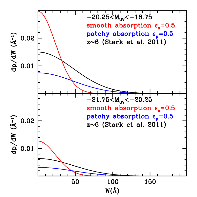
Figure 1: Illustration of our model intrinsic distribution of rest-frame equivalent width $W$. A fit to the distribution measured at $z\sim 6$ by Stark et al. (2011) is shown as a black line. Red and blue lines represent a model with smooth and patchy absorption, respectively.

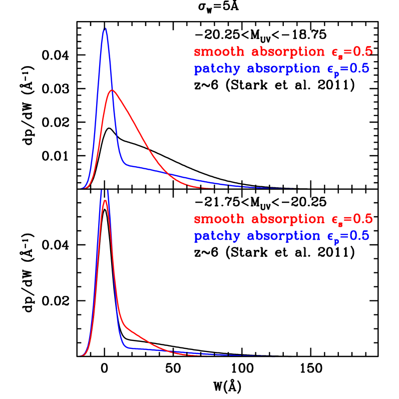
Figure 2: As in Figure 1, including a typical error of 5Å on $W$. Non emitters now introduce a bump for small values of $W$, centered at zero.

The two models describe in a very simple manner two interesting physical scenarios, and illustrate the different strategies required to investigate them. In the patchy model, there are overall fewer emitters than in the smooth model, but they are found at higher equivalent widths. For the examples shown in Figure 1, depending on the sensitivity one can find more sources in either model: above $\sim$50Å, one expects to find more sources in the patchy case; below $\sim$50Å  the smooth model provides more sources.

2.1 Application to spectroscopic data

We now have to connect these distributions to the observables, a set of fluxes measured at different wavelengths $\lambda_{i}$ {$f_{i}=f(\lambda_{i})$}. For simplicity we consider an unresolved emission line, extracted without weighting from N_l pixels, so that the effective noise is the noise measured within a pixel multiplied by $\sqrt{N_{l}}$, while the effective flux is the flux multiplied by $N_{l}$. Thus, the predicted flux is non zero only in the pixel containing the redshifted Lyman $\alpha$ ($\lambda_{0}$) and it is given by:

$$f_{p}(\lambda=(1+z)\lambda_{0})=W(1+z)f_{o}10^{-0.4m}\frac{c}{\lambda_{0}^{2}(1+z)^{2}}\equiv Wf_{m},$$ (4)

where $f_{0}=3.631\cdot 10^{-20}$ erg s^-1 Hz^-1 cm^-2, and the first (1+z) transforms the rest frame equivalent width into observer frame equivalent width. In order to take into account the effects of resolution and line shape, and allow for optimal weighting, it is sufficient to replace the above equation with an appropriate function, e.g. a Gaussian of width equal to the resolution $\sigma_{\lambda}$:

$$f_{p}(\lambda)=\frac{Wf_{m}}{\sqrt{2\pi}\sigma_{\lambda}}e^{-\frac{1}{2}\left(\frac{\lambda-\lambda_{0}}{\sigma_{\lambda}}\right)^{2}}$$ (5)

Doing this correctly would require knowledge of the line profile, and would add an additional convolution and unnecessary computational burden at this stage. Therefore we will adopt the more conservative approach outlined above and do not implement this refinement.

By combining Equations 1-4 with the appropriate Gaussian noise {$\sigma_{i}$}, we can infer the posterior probability of $\epsilon$ (which we use to indicate both $\epsilon_{\rm p}$ and $\epsilon_{\rm s}$) and $z$ given an observed spectrum and continuum magnitude using Bayes’ Theorem:

$$p(\epsilon,z_{i}|\{f\},m)=\frac{1}{Z}\left(\Pi_{i}\int dWp(f_{i},m|W,z_{i})p(W|\epsilon)\right)p(\epsilon)p(z_{i}),$$ (6)

i.e.:

$$p(\epsilon,z_{i}|\{f\},m)=\frac{1}{Z}\int_{0}^{\infty}dW\left(\frac{1}{\sqrt{2\pi}\sigma_{i}}e^{-\frac{1}{2}\left(\frac{f_{i}-Wf_{m}}{\sigma_{i}}\right)^{2}}\right)\Pi_{j\neq i}N(f_{j},\sigma_{j}^{2})p(W|\epsilon)p(\epsilon)p(z_{i})$$ (7)

where $z_{i}=\lambda_{i}/\lambda_{0}-1$, and $N(f_{j},\sigma_{j}^{2})$ is the standard Gaussian (normal) distribution with mean $f_{j}$ and standard deviation $\sigma_{j}$. The likelihood is as usual the probability of obtaining the data for any given value of the parameters $p(\{f\},m|\epsilon,z_{i})=\Pi_{i}p(f_{i},m|\epsilon,z_{i})$, and for simplicity the error on $m$ has been considered negligible. For simplicity we consider independent priors for $\epsilon$ and $z_{i}$, even though one could easily implement a physically motivated prior, where $\epsilon$ depends on $z_{i}$ (i.e. of the form $p(\epsilon|z_{i})p(z_{i})$). The prior p($\epsilon$) is assumed to be uniform between zero and unity, i.e. the intensity of Lyman$\alpha$ cannot increase beyond $z\sim 6$; alternatively one could assume it to be uniform between zero and 1/$A$, which is the maximum value consistent with a probability density function positive everywhere. The prior p($z_{i}$) is given by the photometric redshift. Note that in the case of incomplete wavelength coverage where p($z_{i}$) is non zero, our formalism will take this into account correctly in deriving limits on $\epsilon$ and $z_{i}$.

The normalization constant $Z$ is known as the Bayesian Evidence and quantifies how well the model matches the data. The evidence ratio is a powerful way to perform model selection (e.g. comparing the patchy and smooth models). For a sample of galaxies, for multiple spectra of the same galaxy, the likelihood is just the product of the individual likelihoods, allowing for efficient combination of data of different depths.

Considering the two specific models, the posterior distributions can be derived analytically:

$$p_{p}(\epsilon_{\rm p},z_{i}|\{f,\sigma\},m)=\frac{C}{Z}\left(\frac{A\epsilon_{\rm p}\sigma_{i}\left(1+\rm{erf}(t_{m,p,i})\right)e^{-\frac{1}{2}\left[\left(\frac{f_{i}}{\sigma_{t,p,i}}\right)^{2}-\left(\frac{f_{i}}{\sigma_{i}}\right)^{2}\right]}}{\sigma_{t,p,i}}+(1-A\epsilon_{\rm p})\right)p(z_{i}),$$ (8)

where

$$C\equiv\Pi_{j}\frac{1}{\sqrt{2\pi}\sigma_{j}}e^{-\frac{1}{2}\left(\frac{f_{j}}{\sigma_{j}}\right)^{2}},$$ (9)

is a constant depending only on the dataset,

$$\sigma_{t,p,i}\equiv\sqrt{\sigma_{i}^{2}+f_{m}^{2}(\lambda_{i})W_{c}^{2}},$$ (10)

and

$$t_{m,p,i}\equiv\frac{f_{m}(\lambda_{i})W_{c}f_{i}}{\sqrt{2}\sigma_{i}\sigma_{t,p,i}}.$$ (11)

In the smooth case, the posterior probability distribution function is given by:

$$p_{s}(\epsilon_{\rm p},z_{i}|\{f,\sigma\},m)=\frac{C}{Z}\left(\frac{\sigma_{i}A\left(1+\rm{erf}(t_{m,s,i})\right)e^{-\frac{1}{2}\left[\left(\frac{f_{i}}{\sigma_{t,s,i}}\right)^{2}-\left(\frac{f_{i}}{\sigma_{i}}\right)^{2}\right]}}{\sigma_{t,s,i}}+(1-A)\right)p(z_{i}),$$ (12)

where

$$\sigma_{t,s,i}\equiv\sqrt{\sigma_{i}^{2}+f_{m}^{2}(\lambda_{i})W_{c}^{2}\epsilon_{\rm s}^{2}},$$ (13)

and

$$t_{m,s,i}\equiv\frac{f_{m}(\lambda_{i})W_{c}f_{i}\epsilon_{\rm s}}{\sqrt{2}\sigma_{i}\sigma_{t,s,i}}.$$ (14)

In the patchy case the posterior pdf is separable and can be integrated analytically to give the posterior pdf for the redshift $z_{i}$

$$p(z_{i}|\{f,\sigma\},m)=\int_{0}^{1}d\epsilon_{\rm p}p(\epsilon_{\rm p},z_{i}|\{f\},m)=$$ (15)

$$=\frac{C}{Z}\left[\frac{A\sigma_{i}\left(1+\rm{erf}(t_{m,p,i})\right)e^{-\frac{1}{2}\left[\left(\frac{f_{i}}{\sigma_{t,p,i}}\right)^{2}-\left(\frac{f_{i}}{\sigma_{i}}\right)^{2}\right]}}{2\sigma_{t,p,i}}+\left(1-\frac{A}{2}\right)\right]p(z_{i}),$$ (16)

A simple illustration of this method applied to simulations is shown in Figure 3. Two emission lines with S/N=5 and S/N=2 have been added to noisy spectra covering the wavelength range 0.947-1.297 $\mu$m (equal to the range covered by our NIRSPEC observations, described in Section 3). We considered this to be a bright galaxy and therefore used A=0.38 and $W_{c}$=47Å. Assuming a prior $p(z)$ appropriate for $Y$-band dropouts, we computed the posterior pdf on $\epsilon$ and $z$. As can be seen from the plots, the S/N=5 detection constrains the redshift exquisitely well (vertical red dashed line), and tends to favor larger values of $\epsilon$, i.e. emitters are common. The S/N=2 weak (non) detection gives a posterior pdf with many spurious peaks in $z$, that are not much higher than the prior distribution, consistent with the fact that the likelihood of a false S/N$>$2 detection is large with $\sim 2000$ pixels. Conversely, since there are no strong lines, the procedure correctly infers that $\epsilon$ should be small. Notice that p($\epsilon$) is clearly non-Gaussian. With only one detection not much can be learned about the distribution of $W$, and therefore the posterior on $\epsilon$ is broad. In Sections 4 and 5 we will consider more informative cases with many sources.

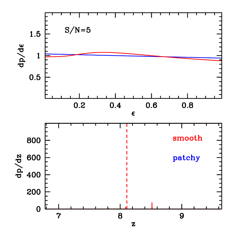
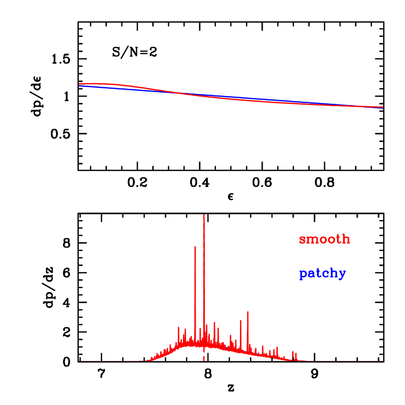
Figure 3: Illustration of inference on simulated data. For a simulated 5$-\sigma$ detection (left panels), the posterior pdf of $z$ (bottom panel) is sharply peaked at the redshift of the emission line (vertical dashed line) independent of the adopted absorption model. As expected, both models prefer large values of $\epsilon$ (top panel). For a simulated weak (non) detection (2$-\sigma$; right panels), there are insignificant noise peaks at several redshifts, on top of the prior $p(z)$, consistent with the many $>$2-$\sigma$ fluctuations expected for a $\sim 2000$ pixel spectrum. As expected, both models prefer small values of $\epsilon$.

In some cases, one might just wish to consider the inference on the parameters if all it is known is that no line has been detected to a certain level of significance, e.g. N$\sigma$. In this case, it is sufficient to consider the integral of the likelihood, so that the posterior pdf becomes in the patchy case:

$$p_{p}(\epsilon_{\rm p},z_{i}|\{\sigma\},N,m)\propto\frac{A\epsilon_{\rm p}\{1+\rm{erf}[N\sigma_{i}/(\sqrt{2}\sigma_{t,p,i})]\}}{1+\rm{erf}(N/\sqrt{2})}\\ +\frac{2A\epsilon_{\rm p}}{\sqrt{2\pi}[1+\rm{erf}(N/\sqrt{2})]}\int_{-\infty}^{N}dx_{i}\rm{erf}(t_{m,p,i})e^{-\frac{1}{2}\left(\frac{x_{i}\sigma_{i}}{\sigma_{t,p,i}}\right)^{2}}+(1-A\epsilon_{\rm p}),$$ (17)

where $t_{m,p,i}$ is only a function of the variable of integration $x_{i}=f_{i}/\sigma_{i}$ and $\sigma_{t,p,i}$ does not depend on $f_{i}$. The proportionality factor is $p(z_{i})C_{N}/Z$, with

$$C_{N}\equiv\Pi_{j}\int_{-\infty}^{N\sigma_{j}}\frac{1}{\sqrt{2\pi}\sigma_{j}}e^{-\frac{1}{2}\left(\frac{f_{j}}{\sigma_{j}}\right)^{2}}=\left[\frac{\left(1+\rm{erf}(N/\sqrt{2})\right)}{2}\right]^{N_{\rm pix}},$$ (18)

for N_pix spectral pixels.

In the smooth case, the posterior pdf is given by:

$$p_{s}(\epsilon_{\rm s},z_{i}|\{\sigma\},N,m)\propto\frac{A\{1+\rm{erf}[N\sigma_{i}/(\sqrt{2}\sigma_{t,s,i})]\}}{1+\rm{erf}(N/\sqrt{2})}\\ +\frac{2A}{\sqrt{2\pi}[1+\rm{erf}(N/\sqrt{2})]}\int_{-\infty}^{N}dx_{i}\rm{erf}(t_{m,s,i})e^{-\frac{1}{2}\left(\frac{x_{i}\sigma_{i}}{\sigma_{t,s,i}}\right)^{2}}+(1-A),$$ (19)

where, again, $t_{m,p,i}$ is only a function of the variable of integration $x_{i}=f_{i}/\sigma_{i}$ and $\sigma_{t,s,i}$ does not depend on $f_{i}$. The constant of proportionality is, as in the patchy case, $p(z_{i})C_{N}/Z$,

2.2 Application to flux catalogs

Often one can only analyze flux catalogs, for example in narrow band searches, or when only noise levels and non-detections are reported by spectroscopic studies. In this case it is useful to consider a simplified treatment, that allows one to combine heterogeneous data in an efficient way. This is achieved by switching from flux to $W$ and by integrating away (marginalize over) the dependency on redshift. In this way, for any detection of an equivalent width $W_{o}$ with noise level $\sigma_{W}$ the likelihoods for the two models are:

$$p_{p}(W_{o}|\epsilon_{\rm p})=\int_{0}^{\infty}dW\frac{1}{\sqrt{2\pi}\sigma_{W}}e^{-\frac{1}{2}\left(\frac{W_{o}-W}{\sigma_{W}}\right)^{2}}\left(\frac{2A\epsilon_{\rm p}}{\sqrt{2\pi}W_{c}}e^{-\frac{1}{2}\left(\frac{W}{W_{c}}\right)^{2}}+(1-A\epsilon_{\rm p})\delta(W)\right)$$ (20)

$$p_{s}(W_{o}|\epsilon_{\rm s})=\int_{0}^{\infty}dW\frac{1}{\sqrt{2\pi}\sigma_{W}}e^{-\frac{1}{2}\left(\frac{W_{o}-W}{\sigma_{W}}\right)^{2}}\left(\frac{2A}{\sqrt{2\pi}\epsilon_{\rm s}W_{c}}e^{-\frac{1}{2}\left(\frac{W}{\epsilon_{\rm s}W_{c}}\right)^{2}}+(1-A)\delta(W)\right).$$ (21)

As in the previous section, the integrals and posterior can be computed analytically. In the patchy case the posterior is given by:

$$p_{p}(\epsilon_{\rm p}|W_{o})=\frac{1}{Z}\left(\frac{A\epsilon_{\rm p}\left(1+\rm{erf}(t_{m,p})\right)e^{-\frac{1}{2}\left(\frac{W_{o}}{\sigma_{W,t,p}}\right)^{2}}}{\sqrt{2\pi}\sigma_{W,t,p}}+\frac{(1-A\epsilon_{\rm p})e^{-\frac{1}{2}\left(\frac{W_{o}}{\sigma_{W}}\right)^{2}}}{\sqrt{2\pi}\sigma_{W}}\right)p(\epsilon_{\rm p}),$$ (22)

where

$$\sigma_{W,t,p}\equiv\sqrt{\sigma_{W}^{2}+W_{c}^{2}}$$ (23)

and

$$t_{m,p}\equiv\frac{W_{c}W_{o}}{\sqrt{2}\sigma\sigma_{W,t,p}}.$$ (24)

In the smooth case, the posterior is given by:

$$p_{s}(\epsilon_{\rm s}|W_{o})=\frac{1}{Z}\left(\frac{A\left(1+\rm{erf}(t_{W,m,s})\right)e^{-\frac{1}{2}\left(\frac{W_{o}}{\sigma_{W,t,s}}\right)^{2}}}{\sqrt{2\pi}\sigma_{W,t,s}}+\frac{(1-A)e^{-\frac{1}{2}\left(\frac{W_{o}}{\sigma_{W}}\right)^{2}}}{\sqrt{2\pi}\sigma_{W}}\right)p(\epsilon_{\rm s}),$$ (25)

where

$$\sigma_{W,t,s}\equiv\sqrt{\sigma_{W}^{2}+W_{c}^{2}\epsilon_{\rm s}^{2}}$$ (26)

and

$$t_{W,m,s}\equiv\frac{W_{o}W_{c}\epsilon_{\rm s}}{\sqrt{2}\sigma\sigma_{W,t,s}}.$$ (27)

If the only information available is about a subset of the wavelength range where the line could possibly be found based on the photometric redshift distribution, this can easily be implemented in this formalism. Assuming for example that the line can be seen only in a range between $z_{\rm min}$ and $z_{\rm max}$, in the patchy case the expression is

$$p_{p}(\epsilon_{\rm p}|W_{o})\propto\left(\frac{A\epsilon_{\rm p}\left(1+\rm{erf}(t_{m,p})\right)e^{-\frac{1}{2}\left(\frac{W_{o}}{\sigma_{W,t,p}}\right)^{2}}}{\sqrt{2\pi}\sigma_{W,t,p}}\frac{(1-A\epsilon_{\rm p})e^{-\frac{1}{2}\left(\frac{W_{o}}{\sigma_{W}}\right)^{2}}}{\sqrt{2\pi}\sigma_{W}}\right)p(z\in[z_{\rm min},z_{\rm max}])\\ +\frac{e^{-\frac{1}{2}\left(\frac{W_{o}}{\sigma_{W}}\right)^{2}}}{\sqrt{2\pi}\sigma_{W}}p(z\notin[z_{\rm min},z_{\rm max}]),$$ (28)

where the constant of proportionality is $p(\epsilon_{\rm p})/Z$. A similar expression applies for the smooth model.

As in the spectroscopic case, for non detections to a certain noise level (e.g. $N\sigma_{W}$) the likelihood is just the integral of the likelihood:

$$p(W_{o}<N\sigma_{W}|\epsilon_{\rm s})=\int_{-\infty}^{N\sigma_{W}}dW_{o}p(W_{o}|\epsilon_{\rm s})$$ (29)

We illustrate the difference between using measurements and upper limits only by means of simulations in Figure 4. We construct a simulated dataset of 99 galaxies drawn from a distribution with $\epsilon_{\rm p}=0.5$, assuming noise $\sigma_{W}=5$Å. In the top panel we perform the inference based only on the detections with significance 5$-\sigma$ or more and counting the other objects as non-detections (using the likelihood in Equation 29). In the bottom panel we used all the available information from the full distribution of measured $W$ (using the likelihoods in Equation 20 and 21 even for fluxes below 5-$\sigma$). In both cases the inference accurately recovers the correct value of $\epsilon_{\rm p}$ and the evidence ratio selects patchy absorption as the best model. However, uncertainties are marginally smaller, and evidence ratio is much more conclusive when one utilizes the full distribution. This underscores the importance of reporting even marginal detections, if possible and if the errors are very well known. If that is not possible, a careful treatment of upper limits is still possible within this framework, and accurate.

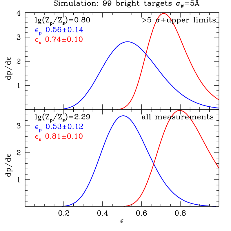
Figure 4: Inference on $\epsilon$ from a simulated sample of 99 objects at $z\sim 8$ with M${}_{\rm UV}<-20.25$. The sample is generated from a distribution of equivalent width with $\epsilon_{\rm p}=0.5$, i.e. equal to that shown in Figure 1, assuming a noise level equivalent to 5Åequivalent width, i.e. 5-$\sigma$ detection limit of 25Å. The top panel illustrates the inference based on counting non-detections and measurements above 5-$\sigma$. The bottom panel utilizes all the information, including non-detections. Both experiments recover the correct value of $\epsilon_{\rm p}$ and strongly prefer the patchy model (by a factor of 6:1 in the upper panel and by 200:1 in the bottom panel). Notice how the inferred value of $\epsilon_{\rm s}$, and the underlying distribution, are dramatically different from the input, illustrating the effects of using the wrong model to interpret the data, without considering evidence for model selection.

3 New observations

3.1 HST photometry and target selection

The photometric data considered in this paper have been obtained as part of the Hubble program GTO/COS 11534 (PI Green), retrieved from the HST archive after the end of their proprietary period. Coordinated parallels in six WFC3 filters where scheduled: three in the UVIS channel (F300X: $4000$ s, F475X: $3200$ s, F600LP $3200$ s) and three in near-IR (F098M: $17229$ s, F125W: $2006$ s, F160W: $2806$ s). The program used the filter set of the HIPPIES survey (Yan et al., 2011) with the addition of F300X and F475X. Compared to the optimized exposure times of our BoRG survey (Trenti et al., 2011a), this set of observations has an integration time in F098M that is about four times longer than necessary to search for $z\sim 8$ galaxies given the depth of the $J$ and $H$ band exposures. Observations were not dithered.

We processed the data using our BoRG pipeline (Trenti et al., 2011a, b). We calibrated individual exposures with calwfc3, then aligned and registered them on a common $0\farcs 08$/pixel scale using multidrizzle (Koekemoer et al., 2002). Sources were detected in the $J$-band image using SExtractor in dual image mode (Bertin & Arnouts, 1996), setting a threshold of at least 9 contiguous pixels with $S/N>0.7$ after normalization of the r.m.s. maps to take into account correlated noise (Trenti et al., 2011a).

To select $z\sim 8$ candidates we require $S/N>8$ for ISOMAG flux in the detection band ($J$) and $S/N>5$ in $H$ (ISOMAG). The standard BoRG near-IR color-color selection has been applied:

$$Y-J\geq 1.75$$ (30)

$$J-H<0.02+0.15\times(Y-H-1.75).$$ (31)

Finally, we require a conservative non-detection in all three optical bands ($S/N<1.5$) for ISOMAG fluxes. Flux measurements are corrected for foreground Galactic extinction using the maps by Schlegel et al. (1998), which reports $A_{B}=0.29$ for the coordinates of the field. Colors are measured using ISOMAG fluxes and have been PSF matched using the latest WFC3 PSF (http://www.stsci.edu/hst/wfc3/ir_ee_model_smov.dat; see also Trenti et al., 2011b).

One source, located at coordinates 22:02:46.33 +18:51:29.5 (J2000) satisfies our selection within the WFC3 field analyzed here. Its photometry is summarized in Table 1. The source is detected with S/N=9.6 in $J$ and S/N=6.9 in $H$ (ISOMAG fluxes) and has a marginal detection in the very deep $Y$ band data (S/N=1.5), with a very red color in the Lyman break filters: $Y-J=2.44^{+1.21}_{-0.60}$ (See Figure 5). The source is clearly resolved in the F125W and F160W images (Figure 5), ruling out contamination by a foreground star.

Table 1: Photometry of $z\sim 8$ candidate.

Filter	magISO	magFIXED	magAUTO
F160W	$26.29\pm 0.15$	$26.51\pm 0.16$	$25.86\pm 0.16$
F125W	$26.01\pm 0.11$	$26.54\pm 0.15$	$25.98\pm 0.16$
F098M	$28.45^{+1.15}_{-0.55}$	$>29.04$	$27.97^{+1.17}_{-0.56}$
F600LP	$>28.46$	$>28.42$	$>27.85$
F475X	$>28.42$	$>28.56$	$>27.82$
F300X	$>27.07$	$>27.21$	$>26.51$

Note. — Photometry for the $z\sim 8$ galaxy candidate discussed in the paper. First column: filter. Second column ISOMAG magnitude, with error. Third column: magnitude within a fixed aperture of radius $r=0\farcs 32$. Fourth column: total magnitude (AUTOMAG). ISOMAG and fixed aperture measurements have been PSF matched to the $J$ band. All measurements have been corrected for galactic reddening using extinction as measured by Schlegel et al. (1998).

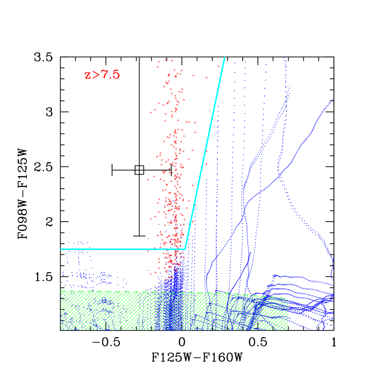
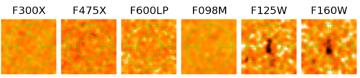
Figure 5: Top panel: Color-color selection for $z\sim 8$ candidates in the BoRG survey (from Trenti et al. 2011a). Red triangles are $z>7.5$ simulated galaxies. Lower redshift contaminants are shown as blue dots (galaxies) and green region (L and T dwarf stars). BoRG11534 (black square with errorbars; ISOMAG colors) is located on the track of $z>7.5$ sources and is well separated from possible contaminants. Lower panels: postage-stamps images ($3\farcs 2\times 3\farcs 2$) in the F300X, F475X, F600LP, F098M, F125W, and F160W bands of BoRG11534 from HST/WFC3 data.

3.2 Keck Spectroscopy

The $Y$-band dropout BoRG11534 (Fig 6) was observed using the NIRSPEC spectrograph (McLean et al., 1998) on the night of August 13 2011. The seeing was excellent ($0\farcs 4$-$0\farcs 5$), and even though part of the night was lost to fog and clouds, we were able to observe the target for 2.5 hrs each in the N1 and N2 setup, covering the wavelength interval 0.9470-1.2969 $\mu$m, corresponding to Lyman $\alpha$ redshifted to z=6.78-9.66, i.e. the range expected for $Y$-band dropouts.

A bright star ($J_{125}=17.78$) was observed in the slit together with the dropout in order to ensure optimal extraction and thus maximize sensitivity, and to provide a secondary spectrophotometric standard, identified as a rK4III star by comparing its colors to those predicted by the Pickles (1998) spectral library (Java applet available at http://lcogt.net/ajp/SpecMatch/hst).

The data were reduced in a standard manner using a set of python scripts. The extracted 1-d spectrum and the noise spectrum are shown in Figure 6. No significant emission is detected. For comparison with other work, we also derive the corresponding flux and equivalent width 5-$\sigma$ limit for an unresolved emission line. The median 5-$\sigma$ limits are $(0.98\pm 0.17)\cdot 10^{-17}$ erg s^-1 cm^-2 and (26$\pm$4) Å in the N1 filter, and $(1.10\pm 0.3)\cdot 10^{-17}$ erg s^-1 cm^-2 and (35$\pm$11) Å in the N2 filter. The error bars represent the 25 and 75 percentile intervals.

The non-detection sets one of the most stringent upper limits to the equivalent width of emission lines for a $Y$-band dropout, and all but rules out faint emission line objects at lower redshifts as a potential contaminant, as in the case of the observations of BoRG58 by Schenker et al. (2011) discussed by Trenti et al. (2011b). In fact, as suggested by Atek et al. (2011), faint emission line objects at appropriate redshifts ([O II] and [O III] or [O III]/H$\beta$ and H$\alpha$) could be mistaken for $z\sim 8$ galaxies when only two detection bands are available. However, if the continuum magnitude in F125W were due to an emission line, it would correspond to $\sim 8\cdot 10^{-17}$ erg s^-1cm^-2, easily detectable with our sensitivity and wavelength coverage. The only exception would be if weak [O III] fell beyond 1.2969$\mu$m ($z>1.590$) but within the F125W filter. In that case however, H$\alpha$ would fall at 1.6999$\mu$m, just outside the F160W filter, and thus would be inconsistent with the detection in $H$.

Figure 6: Keck spectroscopy of $Y$-band dropout BoRG11534. The top panel shows the measured spectrum; the middle panel shows the equivalent 5-$\sigma$ flux limit for an unresolved line; the bottom panel shows the corresponding 5-$\sigma$ equivalent width limit.

4 Current limits

In § 4.1 we apply our methodology to a compilation of published systematic spectroscopic studies of $z^{\prime}$-band dropouts deriving robust constraints on the distribution of Lyman-$\alpha$ emission at $z\sim 7$. Then, in 4.2 we show that existing spectroscopic samples of $Y$-dropouts, including our new upper limit, are not sufficient to constrain the distribution of Lyman-$\alpha$ emission at $z\sim 8$.

4.1 Inference from $z^{\prime}$-band dropouts at $z\sim 7$

In order to obtain an unbiased estimate it is essential to analyze datasets for which detections and non-detections have both been reported. The depth and observational configuration need not be the same, but serendipitous discoveries are difficult to incorporate. For this reason we limit our analysis to three recently published samples of $z^{\prime}$-band dropouts, for which complete information is available (Pentericci et al., 2011; Schenker et al., 2011; Ono et al., 2011). The total sample consists of 39 $z^{\prime}$-band dropouts: 20 objects studied by Pentericci et al. (2011), 11 objects studied by Ono et al. (2011), and the eight objects in the top part of Table 1 of the paper by Schenker et al. (2011) for which deep LRIS spectroscopy is available. Aiming to ensure homogeneity in our constraints at $z\sim 7$ we do not include objects with estimated photo-z above $z=7.5$, or objects for which only NIRSPEC coverage is available. For each object we consider the appropriate measurements or upper limits on line equivalent width as quoted by the authors, and we use the parameters $A$ and $W_{c}$ appropriate for its absolute UV magnitude.

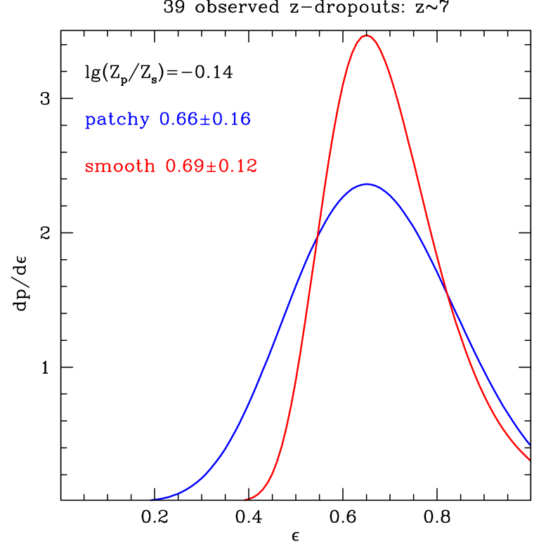
Figure 7: Marginalized posterior distribution function of $\epsilon$ at $z\sim 7$ based on a compilation of 39 $z^{\prime}$-dropouts with deep spectroscopic follow-up taken from the literature (Pentericci et al., 2011; Ono et al., 2011; Schenker et al., 2011). Both the patchy and smooth model indicate clearly that the Lyman $\alpha$ emission is significantly quenched at $z\sim 7$ with respect to $z\sim 6$.

As shown in Figure 7 the data clearly prefer $\epsilon<1$, independent of the model considered. The evidence ratio indicates no significant preference for either model. For the patchy model, we find $\epsilon_{\rm p}=0.66\pm 0.16$. For the smooth model we find $\epsilon_{\rm s}=0.69\pm 0.12$. Our analysis gives consistent results, albeit with larger errors and marginal differences, for each of the subsamples (Ono $\epsilon_{\rm p}=0.75\pm 0.19$, $\epsilon_{\rm s}=0.74\pm 0.15$; Pentericci $\epsilon_{\rm p}=0.59\pm 0.18$, $\epsilon_{\rm s}=0.66\pm 0.14$; Schenker $\epsilon_{\rm p}=0.51\pm 0.25$, $\epsilon_{\rm s}=0.69\pm 0.16$).

In terms of Gaussian approximation of the posterior, $\epsilon=1$ is rejected at more than two standard deviations. An increased fraction of interlopers with respect to analogous samples at $z\sim 6$, could potentially explain this finding. However, assuming a typical fraction of $\sim 25\%$ at $z\sim 6$ (Fontana et al., 2010), would require the fraction of interlopers to be $\sim 50$% at $z\sim 7$, i.e. double. This seems highly unlikely considering that the technique is the same and the quality of the photometry is the same. We thus confirm the finding that the distribution of Lyman $\alpha$ equivalent widths is significantly weaker at $z\sim 7$ with respect to $z\sim 6$ possibly signaling the onset of cosmic reionization (Fontana et al., 2010).

We can give a simple interpretation of our results noticing that $\epsilon$ corresponds to the average excess optical depth of Lyman$\alpha$ with respect to $z\sim 6$, i.e. $\langle e^{-\tau_{\rm Ly\alpha}}\rangle$. Therefore our measurement implies $\langle\tau_{\rm Ly\alpha}\rangle=0.4\pm 0.2$. In order to interpret this number correctly one cannot assume a uniform ionized medium (Miralda-Escudé, 1998), but it is essential to take into account local HII regions, whose size depends on the efficiency of galaxies in producing ionizing photons. Furthermore, it is also essential to take into account clustering, since nearby sources also contribute to the size of the ionized region. In this scenario, we can use the models by Wyithe & Loeb (2005) to connect our observed optical depth to the fraction of neutral hydrogen. The typical luminosity of M${}_{\rm UV}\sim-20$ of the $z\sim 7$ sample, corresponds to a halo mass of $\sim 1.5\cdot 10^{11}$ M_⊙ (Trenti et al., 2010), and therefore a circular velocity of $\sim 170$ kms^-1, and velocity dispersion $\sim 120$ kms^-1. Thus, our measured optical depth falls at the low end of the range predicted by their models at $z\sim 7$, i.e. consistent with a ionized fraction of hydrogen of 0.4-0.7. We note that this result depends critically on the local environment of the galaxies rather than on the average properties of the intergalactic medium, and therefore our conclusions on the fraction of ionized gas should be taken with a grain of salt.

4.2 Inference from $Y$-band dropouts at $z\sim 8$

The situation is much less well-defined at $z\sim 8$ and above. Few reports of deep spectroscopic follow-up of WFC3-selected $Y$-band dropouts are reported in the literature (Schenker et al., 2011), owing to the challenges of near infrared spectroscopy from the ground. Only one detection has been reported to our knowledge by Lehnert et al. (2010), and with unusually high equivalent width, and significance just above the conventional threshold ($S/N\sim 6$). Therefore we do not expect our inference to be conclusive, but nevertheless it is useful to illustrate our current limits, in view of the future studies that we will discuss in the next section.

We begin by analyzing our own non-detection of BoRG11534. For this dataset we can exploit the full spectrum and take advantage of all the available information. The marginalized posterior pdfs are shown in Figure 8. As expected both the redshift and $\epsilon$ parameters are unconstrained by the data.

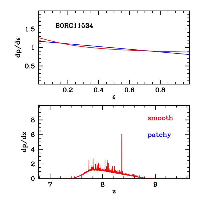
Figure 8: Marginalized posterior distribution functions based on the new observations of BoRG11534, presented in this paper. As expected, the non-detection implies no-constraints on the redshift (the small spike at $z\sim 8.4$ is insignificant and fully expected given the number of pixels; see the right panel of Figure 3), while it implies a very weak preference for small values of $\epsilon$.

We therefore add the two $z\sim 8$ objects from the sample of Schenker et al. (2011) that have complete wavelength coverage from NIRSPEC: A1703_zD7 (Bradley et al., 2011) BoRG58 (which is selected from our BoRG survey; Trenti et al., 2011a). Given the extreme faintness of A1703_zD7, even accounting for lensing magnification, most of the constraints come from the two BoRG targets. To analyze these two objects we use the version of the formalism developed for flux upper limits, adopting the median equivalent width limit over the spectral range, as estimated by scaling our observed noise to the actual exposure time (the instrumental configuration is the same). As expected, the data show a weak preference for small values of $\epsilon$, although clearly the evidence is inconclusive. Note if the fraction of bright lyman-$\alpha$ emitters at $z\sim 6$ were higher than in the sample published by Stark et al. (2011) as recently suggested by Curtis-Lake et al. (2011), the preference for small values of $\epsilon$ would increase, although not significantly given the small sample size at $z\sim 8$.

As a test we also add the detection of the object from Lehnert et al. (2010). Interestingly, consistent with the high equivalent width of the detection, the results are significantly different for the two models. The smooth model is only capable of producing the event for large values of $\epsilon$, while the patchy model can explain the observations with a broader range of parameter values. This is reflected in the evidence, which marginally prefers the patchy model by a factor of 3:1 if the detection is included, while the two models are indistinguishable if the detection is excluded.

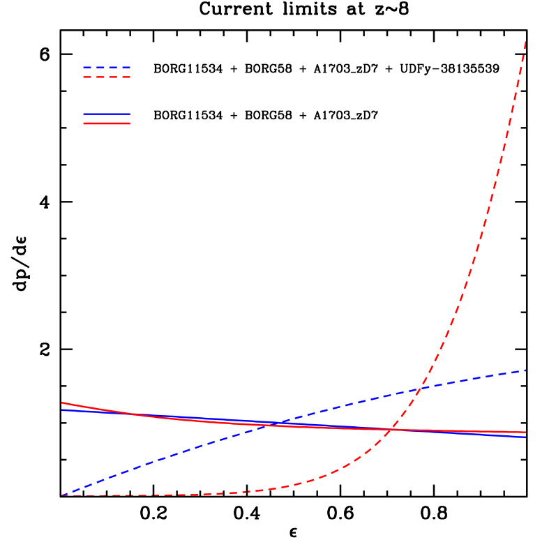
Figure 9: Marginalized posterior distribution function of $\epsilon$ based on the new observations of BoRG11534, as well as the study of three other objects from the literature. As expected, the non-detections imply a very weak preference for small values of $\epsilon$. The addition of the detection of UDFy-38135539 (Lehnert et al., 2010) pushes the inference to larger values of $\epsilon$ the detection is more unlikely under the smooth model which therefore expresses a stronger preference for $\epsilon_{\rm s}\approx=1$, although overall the smooth model is marginally disfavored by the evidence.

4.3 Comparison with previous work

Our results at $z\sim 7$ are based on the deep and comprehensive optical follow-up of $z^{\prime}$-dropouts performed by three groups (Schenker et al., 2011; Ono et al., 2011; Vanzella et al., 2011; Fontana et al., 2010; Pentericci et al., 2011). Although our methodology allows us to determine more than just the fraction of emitters above a certain threshold it is straightforward to compare with the commonly reported fraction of Lyman$\alpha$ emitters above a certain threshold, typically $X^{55}$ and $X^{25}$.

In the patchy model the fraction of Lyman$\alpha$ emitters is simply $X^{W}_{z=7}=\epsilon_{\rm p}X^{W}_{z=6}$, where $X^{W}_{z=6}$ is the reference measurement at $z=6$ (in this case taken from Stark et al. 2011). For the bright subsample we find $X^{25}_{z=7}=\epsilon_{\rm p}(0.20\pm 0.08)=0.14\pm 0.06$ and $X^{55}_{z=7}=\epsilon_{\rm p}(0.074\pm 0.050)=0.05\pm 0.04$. For the faint subsample we find $X^{25}_{z=7}=\epsilon_{\rm p}(0.54\pm 0.11)=0.37\pm 0.11$ and $X^{55}_{z=7}=\epsilon_{\rm p}(0.27\pm 0.08)=0.19\pm 0.07$.

In the smooth model the fraction of Lyman$\alpha$ emitters is $X^{W}_{z=7}=\frac{\rm{erfc}(W/\sqrt{2}\epsilon_{\rm s}W_{c})}{\rm{erfc}(W/\sqrt{2}W_{c})}X^{W}_{z=6}$. Thus, for the bright subsample the smooth model implies $X^{25}_{z=7}=0.14\pm 0.06$ and $X^{55}_{z=7}=0.02\pm 0.02$. For the faint subsample, the smooth model implies $X^{25}_{z=7}=0.38\pm 0.11$ and $X^{55}_{z=7}=0.08\pm 0.03$.

We conclude that the models give mutually consistent emitter fractions within the errors, except for $W>55$Å, where by construction the patchy model has significantly more probability. Below 25Å the converse would be true. More data are needed to distinguish the two models as discussed in the previous section.

The agreement with published data is excellent for the patchy model, which is equivalent to that implicitly assumed by previous authors. However, the slightly different results for the smooth model emphasize that it is important to recognize the inevitable underlying model when analyzing data. Furthermore, our uncertainties are significantly smaller than those quoted by Ono et al. (2011) using virtually the same data, by virtue of our ability to take into account strength and significance of non-detections, rather than just counting detections above a certain threshold. More data are necessary to determine which model is a better description of the data, including of course more general models than the one discussed here.

Finally, we note that our interpretation of the findings in terms of ionized fraction of neutral hydrogen is consistent with that of Pentericci et al. (2011) based on the models by Dijkstra et al. (2011).

5 Forecasts

We conclude by presenting forecasts for observing campaigns of $z\sim 8$ galaxies. Given the paucity of strong emitters among the dropout population it is clear that multiplexing capabilities, such as those afforded by grism spectroscopy using the WFC3-IR channel, or those available or soon to be available from the ground, will be key to make progress. The question is what is the optimal strategy (how deep and how many objects one has to observe) in order to make progress, for example distinguishing the two empirical models introduced in this paper. The simulations shown in Figure 4 give a first answer: by observing 99 objects to the current best limiting depth it should be possible to answer the question definitively. However, finding 99 bright $Y$-band dropouts will require an order of magnitude more survey area than what is planned to be observed so far with WFC3 and considerable effort for follow-up, given their low density on the sky even with clustering (Trenti et al., 2011a, b).

Figures 10 and 11 show the number of detections expected as a function of observed targets, together with the r.m.s. scatter, as measured from Montecarlo simulations. The noise level of the space based observations is uniform and equal to the median value of the ground based observations, and they are given in terms of 5$<\sigma>$ flux limits in units of 10^-17 ergs^-1cm^-2 in the captions. The brighter one is comparable to that achieved by our 2.5hrs-long Keck-NIRSPEC integrations while the fainter one is 5 times more sensitive. The fainter limits can be achieved with realistically long observations with high efficiency IR spectrographs on ground based 8-10m telescopes (e.g. Lehnert et al., 2010, reached $5\cdot 10^{-18}$ergs^-1cm^-2 in 14.8hrs of integration with SINFONI), or with long multi-orbit integrations using the grism mode on WFC3-IR (see,e.g., Atek et al., 2011; Trump et al., 2011). Alternatively, these limits can be readily reached with the aid of moderate lensing magnification, which is commonly found in the field of rich clusters (e.g. Bradač et al., 2009; Hall et al., 2011; Bradley et al., 2008; Richard et al., 2008; Bradley et al., 2011). The detection rate is somewhat higher in general from space, since the sky emission lines cause higher incompleteness in ground based data. A disadvantage of WFC3 grism data is their low spectral resolution, compared to what is generally obtained from the ground, and therefore the inability to infer and use line shape information.

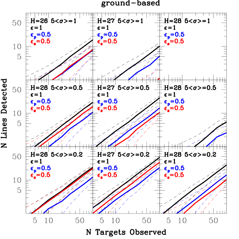
Figure 10: Predicted detection rates for ground based observations of Y-band dropouts as a function of continuum depth and spectroscopic sensitivity. Spectroscopic sensitivity is given in units of 10^-17 erg s^-1 cm^-2. Mean number of detections (solid line) and 1-$\sigma$ confidence contours (dashed lines) are shown for three reference models: 1) $\epsilon=1$ i.e. Lyman$\alpha$ distribution as at $z\sim 6$ (black lines); 2) $\epsilon_{\rm p}=0.5$ (blue lines), i.e. half the emitters as at $z\sim 6$; 3) $\epsilon_{\rm s}=0.5$ (red lines), i.e. half the intensity of emission as at $z\sim 6$.

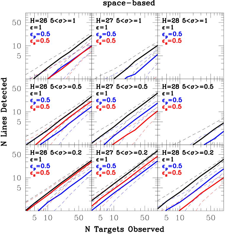
Figure 11: As in Figure 10 for space based observations.

The average number of detected objects is a strong function of both sensitivity and continuum magnitude. By going deeper one targets intrinsically fainter objects, therefore with a higher fraction of emitters, at the price of a higher noise in terms of $W$. In addition the predictions of the patchy and smooth model differ significantly as a function of depth and sensitivity. This is illustrated very clearly in the middle row of Figures 10 and 11. With 5-$\sigma$ sensitivity of $5\cdot 10^{-18}$ erg s^-1cm^-2 at $H=26$ the smooth model yields significantly more detections than the patchy model. Conversely, at $H=27$, the patchy model yields more detections, because the high equivalent width tail dominates at the fainter magnitudes. At $H=28$, one has to go even deeper ($2\cdot 10^{-18}$ erg s^-1cm^-2) to have any realistic chances of detection.

The r.m.s. scatter in the predicted number of detections provides additional insight into future strategies. First, it can be used to estimate the minimum number of targets that one needs to observe to have a detection. Depending on the model and depth of observations, the minimum number of targets required for a detection (with $>84$ probability, i.e. from the 1-$\sigma$ lower limit) varies between a few (for $\epsilon=1$, $H=27$ and depth $0.2$) and virtually infinity for shallower observations at $H=28$. Second, it can be used to estimate the minimum number of targets needed to distinguish between models. At depths comparable to this present study, of order 60 targets are needed to distinguish $\epsilon=1$ from $\epsilon_{\rm p}$ or $\epsilon_{\rm s}=0.5$. In the more favorable case of deeper observations (0.5 depth) at $H=27$, of order 20 targets would be sufficient for that purpose, while $\sim 50$ or more would be needed to start to distinguish between $\epsilon_{\rm p}=0.5$ and $\epsilon_{\rm s}=0.5$.

Clearly, at the moment, we are far from having a number of detections at $z\sim 8$ sufficient to characterize the distribution of Lyman$\alpha$ emission, and in turn the properties of galaxies and the intergalactic medium at that time. However, this goal is within reach in the next few years. To evaluate an efficient strategy we need to consider the density of Y-band dropouts in the sky as a function of magnitude. Those are highly uncertain at this time, especially at the bright end of the luminosity function, therefore we can only consider them as rough estimates. We consider two estimates of the differential number count densities, based on the luminosity function ($\phi_{*}=0.38\cdot 10^{-3}$Mpc^-3; $\alpha=-2.0$; M${}_{*}=-20.3$ Bouwens et al., 2011) and on the observed counts of Bouwens et al. (2011) and on our own estimate from BoRG at the bright end (Trenti et al., 2011a). The lower estimates come from observed number counts and the higher estimates from the luminosity function, i.e. corrected for incompleteness. The resulting differential number count densities are 0.04, 0.3, 1.2, 2.4 arcmin^-2 mag^-1 and 0.05, 0.4, 1.8, 5.4 arcmin^-2 mag^-1, respectively at $H=26,27,28,29$. These densities correspond to roughly 0.18-0.23, 1.4-2.0, 5.6-8.4, 11-26 per WFC3 field of view, and 1.4-1.8, 11-14, 43-65, 86-194 per MOSFIRE field of view (McLean et al., 2010). Thus, in blank fields, WFC3 effectively does not provide any multiplexing advantage until $H\sim 28$, where hope of detection starts at $5\cdot 10^{-18}$ erg s^-1cm^-2. This requires deep $\sim$20 orbits-long integration according to the WFC3 exposure time calculator. Conversely, it is sufficient to reach beyond $H=27$ to start gaining significantly with MOSFIRE, neglecting the positive effects of clustering (Trenti et al., 2011b). Even with moderate gravitational lensing magnification $\mu$ one gains substantially in multiplexing. The gain is especially marked at the bright end, where the number counts are dominated by the exponential part of the luminosity function (e.g. Treu, 2010), and therefore the differential surface density increases as $e^{\mu}/\mu$, i.e. a factor of $\sim 5$ per magnitude. In addition, by effectively going deeper one further gains from the higher fraction of Lyman$\alpha$ emitters amongst the intrinsically fainter population of galaxies (see Figure 1). An accurate estimate of the lensing gain will depend on the details of the gravitational telescope under consideration and is beyond the scope of this paper. In the longer run, the James Webb Space Telescope will be able to detect significantly fainter emission. In eight hours of integration with the G140M grism $10^{-18}$ erg s^-1cm^-2 can be detected at S/N=9. JWST can even detect the continuum of these sources, if Lyman $\alpha$ is completely absent. At AB magnitude $26$ within the G140M grism bandpass, NIRSPEC can detect the continuum with S/N=3 per resolution element in eight hours.

6 Summary

With the goal of understanding the properties of the first galaxies and the intergalactic medium at $z\sim 7$ and above, we have developed a simple yet powerful Bayesian framework to analyze observations of Lyman$\alpha$ in emission. The framework is flexible enough to enable the combination of datasets of different completeness, with different noise properties. In addition, it enables one to take full advantage of the information available.

Within this framework we implement two simple phenomenological models to describe the evolution of the distribution of equivalent widths with respect to a reference distribution, the one measured at $z\sim 6$ by Stark et al. (2011). In the patchy model, equivalent to that considered by previous work (Fontana et al., 2010; Ono et al., 2011; Schenker et al., 2011; Pentericci et al., 2011), Lyman$\alpha$ at $z>6$ is either completely absent or drawn from the $z\sim 6$ distribution (with probability $\epsilon_{\rm p}$). In the smooth model, the distribution of Lyman$\alpha$ is homogeneously reduced by a factor $\epsilon_{\rm s}$. These models can be thought as simple idealizations of patchy and smooth reionization. In the first case, some of the line of sights are completely absorbed by the intergalactic medium, while others are unabsorbed. In the second case, every line of sight is attenuated by the same amount. Clearly, reality is likely to be more complicated, but these two models should bracket somewhat the expected behavior of the IGM near the epoch of reionization and therefore provide useful guidance in planning observations and interpreting data. The parameters $\epsilon_{\rm p}$ and $\epsilon_{\rm s}$ can be physically interpreted as the average excess optical depth of Lyman$\alpha$ with respect to $z\sim 6$, i.e. $\langle e^{-\tau_{Ly\alpha}}\rangle$.

We apply our methodology to a sample of 39 $z\sim 7$ dropouts collected from the literature and to new and published observations of $z\sim 8$ dropouts. Our findings can be summarized as follows:

• At $z\sim 7$ the distribution of Lyman$\alpha$ equivalent width is significantly reduced with respect to $z\sim 6$, consistently for the patchy and smooth model, respectively by factors $\epsilon_{\rm s}=0.69\pm 0.12$ and $\epsilon_{\rm p}=0.66\pm 0.16$. The data do not provide enough information to choose between our two models.

• The models can be used to compute fractions of emitters above any equivalent width $W$ at $z\sim 7$. For $W>25$Å, we find $X^{25}_{z=7}=0.37\pm 0.11$ ($0.14\pm 0.06$) for galaxies fainter (brighter) than M_UV=-20.25 for the patchy model. This is consistent with previous work, but with a smaller uncertainties by virtue of our full use of the data. For the smooth model we find $X^{25}_{z=7}=0.14\pm 0.06$ and $X^{25}_{z=7}=0.38\pm 0.11$, respectively for the bright and faint subsample.

• We observed with the Keck Telescope a bright and spatially resolved Y-band dropout (H$\approx 26$), selected as part of the BoRG survey (Trenti et al., 2011a). We do not detect any emission lines down to a 5$-\sigma$ limit of 10^-17erg s^-1cm^-2. The lack of emission lines eliminates the possibility that this galaxy is a pure emission line object at lower redshifts.

• At $z\sim 8$ we combine our new observations with those of three dropouts observed by Schenker et al. (2011, including one target from our own BoRG Survey) and by Lehnert et al. (2010) and find that the inference is inconclusive.

• We forecast the outcome of future observations of $z\sim 8$ galaxies as a function of continuum magnitude and spectroscopic sensitivity, and show that it is possible to detect Lyman$\alpha$ and start to constrain its distribution by observing several tens of targets.

In conclusion – even though much progress has been made at $z\sim 7$ and on the imaging front at $z\sim 8$ – more spectroscopic data are clearly needed to characterize the elusive population of $z\sim 8$ galaxies and the distribution of Lyman $\alpha$ emission and absorption. Our models show that making progress will require substantial effort, even with sensitivities within reach of the grism mode on board WFC3 and upcoming infrared spectrographs such as MOSFIRE. However, progress is definitely within reach, especially with the assistance of lensing magnification provided by clusters of galaxies used as gravitational telescopes.

Appendix A Alternative parameterization of $z\sim 6$ W distribution

We consider here an alternative parameterization of the distribution of W at $z\sim 6$ and derive the relevant formulae in this case. If, as suggested by (Fontana et al., 2010; Pentericci et al., 2011), the distribution of $W$ for faint sources at $z\sim 6$ has an additional tail of high equivalent width distributions, represented by a uniform distribution out to $W_{m}$=150Å, Equation 1 becomes:

$$p_{6}(W)=\frac{2A}{\sqrt{2\pi}W_{c}}e^{-\frac{1}{2}\left(\frac{W}{W_{c}}\right)^{2}}H(W)+(1-A-B)\delta(W)+\frac{B}{W_{m}}H(W)H(W_{m}-W).$$ (A1)

By fitting the distribution measured by Stark et al. (2011), we find that $A=0.81$, $B=0.05$ and $W_{c}=43$Å provide a good description of the data. $W_{c}$ is somewhat reduced with respect to the default case to counterbalance the extra uniform tail. Then Equations 8 and 12 gain an additional term of the likelihood:

$$p_{pu}(\epsilon_{\rm p},z_{i}|\{f,\sigma\},m)=p_{p}+\frac{C}{2ZW_{m}}\left(B\epsilon_{\rm p}\left(\rm{erfc}(-\frac{f_{i}}{\sqrt{2}\sigma_{i}})-\rm{erfc}(\frac{W_{m}f_{m}-f_{i}}{\sqrt{2}\sigma_{i}})\right)\sqrt{2\pi}\sigma_{i}e^{\frac{1}{2}\left(\frac{f_{i}}{\sigma_{i}}\right)^{2}}\right)p(z_{i}),$$ (A2)

$$p_{su}(\epsilon_{\rm s},z_{i}|\{f,\sigma\},m)=p_{s}+\frac{C}{2ZW_{m}}\left(B\left(\rm{erfc}(-\frac{f_{i}}{\sqrt{2}\sigma_{i}})-\rm{erfc}(\frac{\epsilon_{\rm s}W_{m}f_{m}-f_{i}}{\sqrt{2}\sigma_{i}})\right)\sqrt{2\pi}\sigma_{i}e^{\frac{1}{2}\left(\frac{f_{i}}{\sigma_{i}}\right)^{2}}\right)p(z_{i}),$$ (A3)

where 1-A$\epsilon_{\rm p}$ needs to be replaced with 1-(A+B)$\epsilon_{\rm p}$ and 1-A needs to be replaced with 1-A-B in $p_{p}$ and $p_{s}$.

Similarly for the flux data case, Equations 22 and 25 become:

$$p_{pu}(\epsilon_{\rm p}|W_{o})=p_{p}+\frac{B\epsilon_{\rm p}}{2ZW_{m}}\left(\rm{erfc}(-\frac{W_{o}}{\sqrt{2}\sigma_{W}})-\rm{erfc}(\frac{W_{m}-W_{o}}{\sqrt{2}\sigma_{W}})\right)p(\epsilon_{\rm p}),$$ (A4)

$$p_{su}(\epsilon_{\rm s}|W_{o})=p_{s}+\frac{B}{2ZW_{m}}\left(\rm{erfc}(-\frac{W_{o}}{\sqrt{2}\sigma_{W}})-\rm{erfc}(\frac{\epsilon_{\rm s}W_{m}-W_{o}}{\sqrt{2}\sigma_{W}})\right)p(\epsilon_{\rm s})$$ (A5)

where again 1-A$\epsilon_{\rm p}$ needs to be replaced with 1-(A+B)$\epsilon_{\rm p}$ and 1-A needs to be replaced with 1-A-B in $p_{p}$ and $p_{s}$.

As a test, we repeat the inference on $z\sim 7$ galaxies using this modified distribution of W for faint galaxies at $z\sim 6$. The results are shown in Figure 12 are well within the errors of the inference with our default choice. The evidence ratio does not express a preference for the default choice or the one with the extra uniform tail (evidence ratio $<0.12$ dex between).

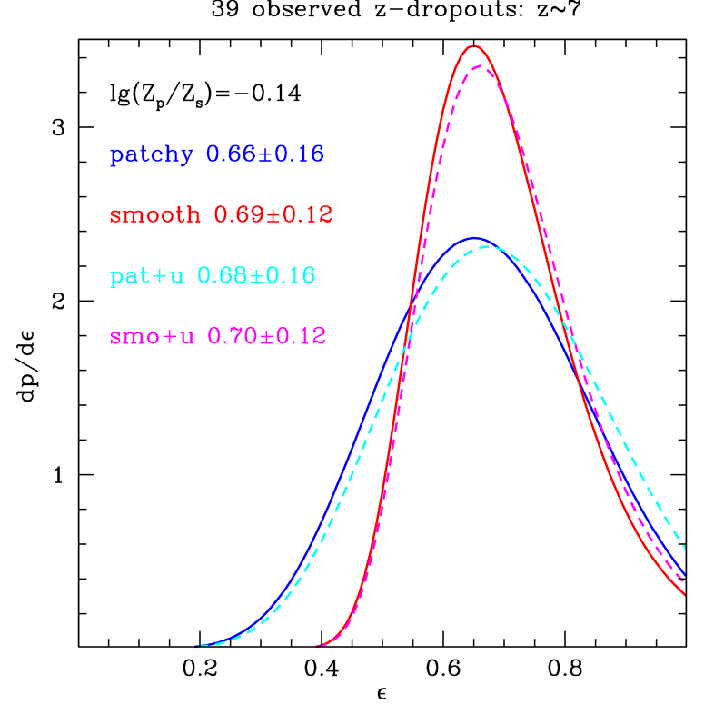
Figure 12: As Figure 7, with the addition of two models that include a uniform tail extending to W=150Å for faint galaxies at $z\sim 6$ (magenta and cyan dashed lines). Our conclusions are unchanged.

References

- Atek et al. (2011) Atek, H., Siana, B., Scarlata, C., Malkan, M., McCarthy, P., Teplitz, H., Henry, A., Colbert, J., Bridge, C., Bunker, A. J., Dressler, A., Fosbury, R., Hathi, N. P., Martin, C., Ross, N. R., & Shim, H. 2011, ArXiv 1109.0639
- Bertin & Arnouts (1996) Bertin, E. & Arnouts, S. 1996, A&AS, 117, 393
- Bolton & Haehnelt (2007) Bolton, J. S. & Haehnelt, M. G. 2007, MNRAS, 382, 325
- Bouwens et al. (2011) Bouwens, R. J., Illingworth, G. D., Oesch, P. A., Labbé, I., Trenti, M., van Dokkum, P., Franx, M., Stiavelli, M., Carollo, C. M., Magee, D., & Gonzalez, V. 2011, ApJ, 737, 90
- Bradač et al. (2009) Bradač, M., Treu, T., Applegate, D., Gonzalez, A. H., Clowe, D., Forman, W., Jones, C., Marshall, P., Schneider, P., & Zaritsky, D. 2009, ApJ, 706, 1201
- Bradley et al. (2008) Bradley, L. D., Bouwens, R. J., Ford, H. C., Illingworth, G. D., Jee, M. J., Benítez, N., Broadhurst, T. J., Franx, M., Frye, B. L., Infante, L., Motta, V., Rosati, P., White, R. L., & Zheng, W. 2008, ApJ, 678, 647
- Bradley et al. (2011) Bradley, L. D., Bouwens, R. J., Zitrin, A., Smit, R., Coe, D., Ford, H. C., Zheng, W., Illingworth, G. D., Benítez, N., & Broadhurst, T. J. 2011, ArXiv 1104.2035
- Castellano et al. (2010a) Castellano, M., Fontana, A., Boutsia, K., Grazian, A., Pentericci, L., Bouwens, R., Dickinson, M., Giavalisco, M., Santini, P., Cristiani, S., Fiore, F., Gallozzi, S., Giallongo, E., Maiolino, R., Mannucci, F., Menci, N., Moorwood, A., Nonino, M., Paris, D., Renzini, A., Rosati, P., Salimbeni, S., Testa, V., & Vanzella, E. 2010a, A&A, 511, A20+
- Castellano et al. (2010b) Castellano, M., Fontana, A., Paris, D., Grazian, A., Pentericci, L., Boutsia, K., Santini, P., Testa, V., Dickinson, M., Giavalisco, M., Bouwens, R., Cuby, J.-G., Mannucci, F., Clément, B., Cristiani, S., Fiore, F., Gallozzi, S., Giallongo, E., Maiolino, R., Menci, N., Moorwood, A., Nonino, M., Renzini, A., Rosati, P., Salimbeni, S., & Vanzella, E. 2010b, A&A, 524, A28+
- Clément et al. (2011) Clément, B., Cuby, J. ., Courbin, F., Fontana, A., Freudling, W., Fynbo, J., Gallego, J., Hibon, P., Kneib, J. ., Le Fèvre, O., Lidman, C., McMahon, R., Milvang-Jensen, B., Moller, P., Moorwood, A., Nilsson, K. K., Pentericci, L., Venemans, B., Villar, V., & Willis, J. 2011, ArXiv 1105.4235
- Curtis-Lake et al. (2011) Curtis-Lake, E., McLure, R. J., Pearce, H. J., et al. 2011, arXiv:1110.1722
- Dayal & Ferrara (2011) Dayal, P. & Ferrara, A. 2011, ArXiv 1109.0297
- Dijkstra et al. (2011) Dijkstra, M., Mesinger, A., & Wyithe, J. S. B. 2011, MNRAS, 414, 2139
- Dijkstra & Wyithe (2011) Dijkstra, M., & Wyithe, S. 2011, arXiv:1108.3840
- Fan et al. (2006) Fan, X., Strauss, M. A., Becker, R. H., White, R. L., Gunn, J. E., Knapp, G. R., Richards, G. T., Schneider, D. P., Brinkmann, J., & Fukugita, M. 2006, AJ, 132, 117
- Fontana et al. (2010) Fontana, A., Vanzella, E., Pentericci, L., Castellano, M., Giavalisco, M., Grazian, A., Boutsia, K., Cristiani, S., Dickinson, M., Giallongo, E., Maiolino, R., Moorwood, A., & Santini, P. 2010, ApJ, 725, L205
- Furlanetto et al. (2006) Furlanetto, S. R., McQuinn, M., & Hernquist, L. 2006, MNRAS, 365, 115
- Hall et al. (2011) Hall, N., Bradac, M., Gonzalez, A. H., Treu, T., Clowe, D., Jones, C., Stiavelli, M., Zaritsky, D., Cuby, J.-G., & Clement, B. 2011, ArXiv 1101.4677
- Hu et al. (2010) Hu, E. M., Cowie, L. L., Barger, A. J., et al. 2010, ApJ, 725, 394
- Iliev et al. (2006) Iliev, I. T., Mellema, G., Pen, U.-L., Merz, H., Shapiro, P. R., & Alvarez, M. A. 2006, MNRAS, 369, 1625
- Kashikawa et al. (2006) Kashikawa, N., Shimasaku, K., Malkan, M. A., et al. 2006, ApJ, 648, 7
- Koekemoer et al. (2002) Koekemoer, A. M., Fruchter, A. S., Hook, R. N., & Hack, W. 2002, in The 2002 HST Calibration Workshop : Hubble after the Installation of the ACS and the NICMOS Cooling System, ed. S. Arribas, A. Koekemoer, & B. Whitmore, 337–+
- Komatsu et al. (2011) Komatsu, E., Smith, K. M., Dunkley, J., Bennett, C. L., Gold, B., Hinshaw, G., Jarosik, N., Larson, D., Nolta, M. R., Page, L., Spergel, D. N., Halpern, M., Hill, R. S., Kogut, A., Limon, M., Meyer, S. S., Odegard, N., Tucker, G. S., Weiland, J. L., Wollack, E., & Wright, E. L. 2011, ApJS, 192, 18
- Lehnert et al. (2010) Lehnert, M. D., Nesvadba, N. P. H., Cuby, J.-G., Swinbank, A. M., Morris, S., Clément, B., Evans, C. J., Bremer, M. N., & Basa, S. 2010, Nature, 467, 940
- Lorenzoni et al. (2011) Lorenzoni, S., Bunker, A. J., Wilkins, S. M., Stanway, E. R., Jarvis, M. J., & Caruana, J. 2011, MNRAS, 414, 1455
- McLean et al. (1998) McLean, I. S., Becklin, E. E., Bendiksen, O., Brims, G., Canfield, J., Figer, D. F., Graham, J. R., Hare, J., Lacayanga, F., Larkin, J. E., Larson, S. B., Levenson, N., Magnone, N., Teplitz, H., & Wong, W. 1998, in Society of Photo-Optical Instrumentation Engineers (SPIE) Conference Series, Vol. 3354, Society of Photo-Optical Instrumentation Engineers (SPIE) Conference Series, ed. A. M. Fowler, 566–578
- McLean et al. (2010) McLean, I. S., Steidel, C. C., Epps, H., Matthews, K., Adkins, S., Konidaris, N., Weber, B., Aliado, T., Brims, G., Canfield, J., Cromer, J., Fucik, J., Kulas, K., Mace, G., Magnone, K., Rodriguez, H., Wang, E., & Weiss, J. 2010, in Society of Photo-Optical Instrumentation Engineers (SPIE) Conference Series, Vol. 7735, Society of Photo-Optical Instrumentation Engineers (SPIE) Conference Series
- McQuinn et al. (2007) McQuinn, M., Lidz, A., Zahn, O., Dutta, S., Hernquist, L., & Zaldarriaga, M. 2007, MNRAS, 377, 1043
- Miralda-Escudé (1998) Miralda-Escudé, J., 1998, ApJ, 501, 15
- Ono et al. (2011) Ono, Y., Ouchi, M., Mobasher, B., Dickinson, M., Penner, K., Shimasaku, K., Weiner, B. J., Kartaltepe, J. S., Nakajima, K., Nayyeri, H., Stern, D., Kashikawa, N., & Spinrad, H. 2011, ArXiv 1107.3159
- Ouchi et al. (2010) Ouchi, M., Shimasaku, K., Furusawa, H., et al. 2010, ApJ, 723, 869
- Pentericci et al. (2011) Pentericci, L., Fontana, A., Vanzella, E., Castellano, M., Grazian, A., Dijkstra, M., Boutsia, K., Cristiani, S., Dickinson, M., Giallongo, E., Giavalisco, M., Maiolino, R., Moorwood, A., & Santini, P. 2011, ArXiv 1107.1376
- Pickles (1998) Pickles, A. J. 1998, PASP, 110, 863
- Richard et al. (2008) Richard, J., Stark, D. P., Ellis, R. S., George, M. R., Egami, E., Kneib, J.-P., & Smith, G. P. 2008, ApJ, 685, 705
- Robertson et al. (2010) Robertson, B. E., Ellis, R. S., Dunlop, J. S., McLure, R. J., & Stark, D. P. 2010, Nature, 468, 49
- Schenker et al. (2011) Schenker, M. A., Stark, D. P., Ellis, R. S., Robertson, B. E., Dunlop, J. S., McLure, R. J., Kneib, J. ., & Richard, J. 2011, ArXiv 1107.1261
- Schlegel et al. (1998) Schlegel, D. J., Finkbeiner, D. P., & Davis, M. 1998, ApJ, 500, 525
- Shin et al. (2008) Shin, M.-S., Trac, H., & Cen, R. 2008, ApJ, 681, 756
- Shull & Venkatesan (2008) Shull, J. M. & Venkatesan, A. 2008, ApJ, 685, 1
- Stark et al. (2011) Stark, D. P., Ellis, R. S., & Ouchi, M. 2011, ApJ, 728, L2+
- Stark et al. (2007) Stark, D. P., Ellis, R. S., Richard, J., Kneib, J.-P., Smith, G. P., & Santos, M. R. 2007, ApJ, 663, 10
- Steidel et al. (1996) Steidel, C. C., Giavalisco, M., Pettini, M., Dickinson, M., & Adelberger, K. L. 1996, ApJ, 462, L17+
- Stiavelli (2009) Stiavelli, M. 2009, From First Light to Reionization: The End of the Dark Ages, ed. Stiavelli, M.
- Stiavelli et al. (2004) Stiavelli, M., Fall, S. M., & Panagia, N. 2004, ApJ, 600, 508
- Trenti et al. (2011a) Trenti, M., Bradley, L. D., Stiavelli, M., Oesch, P., Treu, T., Bouwens, R. J., Shull, J. M., MacKenty, J. W., Carollo, C. M., & Illingworth, G. D. 2011a, ApJ, 727, L39+
- Trenti et al. (2011b) Trenti, M., Bradley, L. D., Stiavelli, M., Shull, J. M., Oesch, P., Bouwens, R. J., Munoz, J. A., Romano-Diaz, E., Treu, T., Shlosman, I., & Carollo, C. M. 2011b, ArXiv 1110.0468
- Trenti et al. (2010) Trenti, M., Stiavelli, M., Bouwens, R. J., Oesch, P., Shull, J. M., Illingworth, G. D., Bradley, L. D., & Carollo, C. M. 2010, ApJ, 714, L202
- Treu (2010) Treu, T. 2010, ARA&A, 48, 87
- Trump et al. (2011) Trump, J. R., Weiner, B. J., Scarlata, C., Kocevski, D. D., Bell, E. F., McGrath, E. J., Koo, D. C., Faber, S. M., Laird, E. S., Mozena, M., Rangel, C., Yan, R., Yesuf, H., Atek, H., Dickinson, M., Donley, J. L., Dunlop, J. S., Ferguson, H. C., Finkelstein, S. L., Grogin, N. A., Hathi, N. P., Juneau, S., Kartaltepe, J. S., Koekemoer, A. M., Nandra, K., Newman, J. A., Rodney, S. A., Straughn, A. N., & Teplitz, H. I. 2011, ArXiv 1108.6075
- Vanzella et al. (2011) Vanzella, E., Pentericci, L., Fontana, A., Grazian, A., Castellano, M., Boutsia, K., Cristiani, S., Dickinson, M., Gallozzi, S., Giallongo, E., Giavalisco, M., Maiolino, R., Moorwood, A., Paris, D., & Santini, P. 2011, ApJ, 730, L35+
- Yan et al. (2011) Yan, H., Yan, L., Zamojski, M. A., Windhorst, R. A., McCarthy, P. J., Fan, X., Röttgering, H. J. A., Koekemoer, A. M., Robertson, B. E., Davé, R., & Cai, Z. 2011, ApJ, 728, L22+
- Wyithe & Loeb (2005) Wyithe, J. S. B. & Loeb, A. 2005, ApJ, 625, 1