The Soft-Collinear Bootstrap:
$\mathcal{N}=4$ Yang-Mills Amplitudes at Six- and Seven-Loops

Abstract

Infrared divergences in scattering amplitudes arise when a loop momentum $\ell$ becomes collinear with a massless external momentum $p$. In gauge theories, it is known that the $L$-loop logarithm of a planar amplitude has much softer infrared singularities than the $L$-loop amplitude itself. We argue that planar amplitudes in ${\cal N}=4$ super-Yang-Mills theory enjoy softer than expected behavior as $\ell\parallel p$ already at the level of the integrand. Moreover, we conjecture that the four-point integrand can be uniquely determined, to any loop-order, by imposing the correct soft-behavior of the logarithm together with dual conformal invariance and dihedral symmetry. We use these simple criteria to determine explicit formulae for the four-point integrand through seven-loops, finding perfect agreement with previously known results through five-loops. As an input to this calculation, we enumerate all four-point dual conformally invariant (DCI) integrands through seven-loops, an analysis which is aided by several graph-theoretic theorems we prove about general DCI integrands at arbitrary loop-order. The six- and seven-loop amplitudes receive non-zero contributions from 229 and 1873 individual DCI diagrams respectively.

PDF and Mathematica files with all of our results are provided at http://goo.gl/qIKe8

1 Introduction

It has long been appreciated that direct Feynman diagram calculations are often a very inefficient way to study multi-loop scattering amplitudes, especially in a theory as simple as planar ${\cal N}=4$ super-Yang-Mills (SYM) theory. Rather, one usually aims first to obtain a representation of a desired amplitude as a linear combination of a (hopefully) small number of (hopefully) relatively simple integrals. To date there have been at least four essentially different technologies available for determining an integral representation for an amplitude. In this paper we introduce a new approach which is both conceptually simple and computationally powerful, as we demonstrate by using it to determine the seven-loop four-particle integrand in SYM theory.

1.1 Brief Review of Four Paths Towards Integral Representations

The most conventional approach is to begin with a collection of integrands, make the ansatz that the amplitude should be a linear combination of those integrals, and then determine the coefficients of the integrands by matching various data—such as generalized unitarity cuts Bern:1994cg ; Bern:1994zx ; Bern:2007ct or leading singularities Buchbinder:2005wp ; Cachazo:2008vp ; Cachazo:2008hp ; Spradlin:2008uu ; Spradlin:1900zz —between the ansatz and the amplitude. Each ‘data point’ generates a linear equation on the coefficients, so for sufficiently many data points, and a sufficiently large set of linearly independent integrands, one can obtain a unique solution for the coefficients. Actually establishing the correctness of the resulting ansatz (i.e., ruling out the possibility of additional contributions to the amplitude which happen to vanish on all of the data points considered) usually requires careful analysis, for example via more complicated $D$-dimensional unitarity cuts. Details of this tried and true approach can be found in the review Bern:2011qt , and we have learned that its power has been exploited in as yet unpublished work to construct an integral representation for the four-particle amplitude at six-loops unpublished_six_loop .

A very different approach has been introduced in CaronHuot:2010zt ; Boels:2010nw , in particular in ArkaniHamed:2010kv , where a relation was presented which allows one (in principle) to write down the integrand of any desired multi-loop amplitude in SYM theory recursively in terms of lower-loop integrands (involving successively more particles). Note that we distinguish here between the integrand, which is a uniquely-defined rational function of internal and external kinematic data in any planar theory, and an integral representation, which is understood to be well-defined only modulo the addition of terms which integrate to zero.

A third even more recent approach relies on the duality, or equivalence, between certain correlation functions in SYM theory and maximally helicity violating (MHV) scattering amplitudes at the level of the integrand Eden:2010zz . Aspects of this duality have been studied in several papers including Alday:2010zy ; Eden:2010ce ; Eden:2011yp ; Eden:2011ku . For the special case of four particles the relevant correlation functions possess an extra hidden symmetry which has been exploited to provide a slick derivation of the four-particle integrand at three-loops in Eden:2011we , and at higher loops in Eden:2012tu .

A fourth approach makes use of the understanding of how soft- and collinear-infrared singularities factorize and exponentiate in planar gauge theory Akhoury:1978vq ; Mueller:1979ih ; Collins:1980ih ; Sen:1982bt ; Sterman:1986aj ; Catani:1989ne ; Collins:1989bt ; Magnea:1990zb ; Catani:1990rp ; Giele:1991vf ; Kunszt:1994np ; Catani:1998bh ; Vogt:2000ci ; Sterman:2002qn . If we restrict for simplicity our attention to MHV amplitudes and denote by $M^{(L)}_{n}=A^{(L)}_{n}/A^{(0)}_{n}$ the ratio of the $L$-loop $n$-particle MHV (color-stripped, partial) amplitude to the corresponding tree amplitude, then exponentiation implies that in dimensional regularization with $D=4-2\epsilon$ we have

$$\log\left[1+\lambda M^{(1)}_{n}+\lambda^{2}M^{(2)}_{n}+\cdots\right]={\cal O}(\epsilon^{-2}),$$ (1)

even though the individual contributions on the left-hand side have stronger infrared (IR) singularities, $M^{(L)}_{n}={\cal O}(\epsilon^{-2L})$. The general form of this statement is regulator-independent: for example, in the Higgs regulator of Alday:2009zm , the right-hand side of eqn. (1) would be ${\cal O}(\log^{2}m)$ while each individual $M^{(L)}_{n}$ diverges as ${\cal O}(\log^{2L}m)$ as the mass is taken to zero—a fact which has been used to guide the construction of various integrands in the Higgs-regularized theory Henn:2010bk ; Henn:2010ir .

The divergent behavior of equation (1) has often been used as an important consistency check on the correctness of integral representations Bern:2006vw ; Cachazo:2006tj ; Bern:2006ew ; Bern:2008ap ; Cachazo:2008hp ; Spradlin:2008uu . Moreover it can be used to guide the construction of a representation for an $L$-loop amplitude by using the requirement that all of the ${\cal O}(\epsilon^{-2L})$ through ${\cal O}(\epsilon^{-3})$ poles must cancel as ‘data’ in the same sense as described above. For example, for the four-particle amplitude at three-loops, if one starts with the one- and two-loop amplitudes as given, and makes the ansatz that $M_{4}^{(3)}$ should be a linear combination of the three-loop ladder and tennis court diagrams, then their coefficients can be uniquely fixed by requiring that eqn. (1) should hold at order $\lambda^{3}$. In this case, the resulting ansatz agrees with the correct three-loop amplitude found in Bern:2005iz , though in general this approach is not guaranteed to work, since it cannot detect the contribution from any individual integral whose infrared behavior is too soft.

1.2 Preview of a New Path Towards Integrands

The last approach outlined above has the obvious disadvantage that it relies upon explicit evaluation of multi-loop integrals, a problem which—despite recent progress—remains extremely difficult in general. In this paper we explore an approach which amounts essentially to imposing eqn. (1) at the level of the integrand, which allows us to work with simple rational functions instead of complicated polylogarithm functions. (Indeed it has been noted in Drummond:2010mb that soft limits can also be handled very easily at the level of the integrand, in particular an $(n+1)$-particle integrand should reduce directly to an $n$-particle integrand in the soft limit $p_{n}\to 0$. This statement is not generally true for integrals due to IR-divergences.)

Infrared divergences arise when some loop momentum becomes collinear with an external momentum $p_{a}$. In terms of the dual coordinates $x_{a}$ defined by $p_{a}=x_{a+1}-x_{a}$ this happens whenever some loop integration variable $x_{A}$ approaches the line connecting $x_{a}$ and $x_{a+1}$ for some $a$ (see ArkaniHamed:2010kv ; ArkaniHamed:2010gh for a detailed discussion). If we take a limit where both $(x_{a}-x_{A})^{2}$ and $(x_{a+1}-x_{A})^{2}$ are order $\epsilon$ (but making sure that all other kinematic invariants take generic, non-vanishing values) then any integrand will have a $1/\epsilon^{2}$ pole in the limit $\epsilon\to 0$. However, we claim that the integrand of the logarithm of any amplitude has only a $1/\epsilon$ pole at any loop-order $L>1$. This phenomenon is clearly related to the fact of eqn. (1), but at the moment we present this claim only as an empirical observation which we have verified for the four-point integrand through seven loop-order.

Assuming that this behavior holds for all $L$, then it obviously can be used as a powerful tool for constructing integrands of amplitudes. We simply need to postulate a suitable basis of integrands for any desired amplitude and try to find a linear combination for which the ${\cal O}(1/\epsilon^{2})$ poles cancel. We call this procedure the soft-collinear bootstrap because it allows the determination of an $L$-loop integrand given all of the corresponding integrands at loop-order $<L$, which appear in the $L$-loop logarithm. (This approach has a similar flavor to the work of ref. Bargheer:2009qu , where it was argued that all tree-level amplitudes could be fully constrained by their collinear singularities, combined with the requirement of Yangian symmetry).

The case of four particles is special because a very simple basis naturally suggests itself: the collection of integrands which are invariant under conformal transformations on the dual $x$ variables, appropriately called dual conformally invariant (DCI) integrands Drummond:2007cf ; Drummond:2007au . This class of integrands has already played an important role in guiding the construction of integral representations at four- Bern:2006ew and five-loops Bern:2007ct . We have checked through seven-loops that the family of DCI integrands at each loop-order is linearly independent (if one imposes dihedral symmetry in the external particles, which is a symmetry of all superamplitudes; it is curious to note that imposing mere cyclic symmetry is sufficient to fix the amplitude through five-loops, but the full dihedral symmetry must be imposed in order to obtain the six- and seven-loop amplitudes). Moreover they remain linearly independent even after picking-off from each one just the residue of its $1/\epsilon^{2}$ pole. Taken together, we are therefore led to conjecture that the four-point integrand can be uniquely determined, to any loop-order, by imposing the ${\cal O}(1/\epsilon)$ collinear behavior together with dual conformal invariance and dihedral symmetry.

It is of course well-known that the four-point amplitude in SYM theory is trivial, in the sense that its logarithm is determined exactly by the anomalous dual conformal Ward identity Drummond:2007au up to an overall multiplicative factor of the cusp anomalous dimension $f(\lambda)$ Korchemsky:1985xj , whose value is in turn known exactly from other considerations Beisert:2006ez . However, since $f(\lambda)$ can obviously be computed by simply integrating the integrand, it is amusing to note that while (anomalous) dual conformal invariance of the logarithm of the amplitude is not powerful enough to fix $f(\lambda)$ alone, our results suggest that dual conformal invariance of the integrand is, when one also imposes the mild ${\cal O}(1/\epsilon)$ collinear behavior together with dihedral symmetry with respect to the external particles. Moreover despite the triviality of the amplitude, the integrand of its logarithm is of independent interest since it is evidently a nontrivial function which makes other remarkable appearances, for example as a Wilson loop expectation value in twistor space Mason:2010yk ; CaronHuot:2010ek ; Belitsky:2011zm ; Adamo:2011pv and as (the square root of) a certain correlation function of stress tensor multiplets Alday:2010zy ; Eden:2010zz ; Eden:2010ce ; Eden:2011yp ; Eden:2011ku .

In section 2 we review important facts and conventions related to integrands in SYM theory and present our main conjectures (all of which we have verified through seven-loops). In section 3 we explain the classification of DCI diagrams, which we use as a basis for constructing the four-particle integrands. Our results are presented and discussed in section 4, and the reader may find more information at four_point_multiloop_datafiles .

Throughout this paper we use the momentum twistor parameterization Hodges:2009hk . Consequently all momenta (both internal and external) are strictly four-dimensional and so all Gram determinant conditions are automatically satisfied. However we suspect that when expressed in terms of the $x$’s, formulae for four-point integrands are actually valid for planar SYM theory in any number of dimensions, a property which is known to hold at least through four-loops Bern:2010tq .

All of the important ingredients in this paper, including the exponentiation of infrared divergences and dual conformal invariance, rely crucially on planarity, but it would clearly be of great interest if some variant of our approach might be applicable beyond the planar limit. Integral representations for the complete four-point amplitude in SYM theory, including all non-planar contributions, are known through four-loops (see for example Bern:2012uf ).

2 Conventions and Conjectures

2.1 The Integrand

The integrand of the four-point amplitude $M_{4}^{(L)}=A_{4}^{(L)}/A_{4}^{(0)}$ in planar SYM theory is, at $L$-loop-order, a rational function involving only the scalar quantities

$$x_{ab}=(x_{a}-x_{b})^{2},\qquad\mathrm{with}\qquad s\equiv x_{24}\quad\mathrm{and}\quad t\equiv x_{13}$$ (2)

formed from the dual coordinates $x_{1},x_{2},x_{3},x_{4}$ associated with the external kinematics and the $L$ loop integration variables $x_{A},x_{B},\ldots$. For example at one and two-loops we have Green:1982sw ; Anastasiou:2003kj

$$M_{4}^{(1)}(x_{A}) =\frac{x_{13}x_{24}}{x_{1A}x_{2A}x_{3A}x_{4A}}\,,$$ (3)

$$M_{4}^{(2)}(x_{A},x_{B}) =\frac{x_{13}^{2}x_{24}}{x_{1A}x_{1B}x_{2B}x_{3A}x_{3B}x_{4A}x_{AB}}+\frac{x_{13}x_{24}^{2}}{x_{1B}x_{2A}x_{2B}x_{3A}x_{4A}x_{4B}x_{AB}}+(A\leftrightarrow B)\,.$$ (4)

In order to avoid a little bit of clutter we omit throughout this paper the somewhat conventional overall prefactors of $(-1/2)^{L}$ and $1/L!$—the latter from symmetrization with respect to the loop integration variables, and the former coming from a choice of how to normalize the measure of integration. In the interest of specificity, let us note that to compute amplitudes in the normalization convention of for example Anastasiou:2003kj our $L$-loop integrands should be integrated with the measure

$$\left(-\frac{1}{2}\right)^{L}\frac{1}{L!}\int\prod_{k=1}^{L}\frac{d^{4}x_{A_{k}}}{i\pi^{2}}\,.$$ (5)

The above examples exhibit three important general properties of integrands:

1. full permutation symmetry $\mathfrak{s}_{L}$ in the $L$ integration variables $x_{A},x_{B},\ldots$;

2. dihedral symmetry $D_{4}$ in the external variables $x_{1},\ldots,x_{4}$;

3. and the absence of double poles.

2.2 The Integrand of the Logarithm

The above properties ensure that there is no ambiguity in defining the integrand of the logarithm of an amplitude. Taylor-expanding the left-hand side of eqn. (1) to seventh-order in $\lambda$, we have

$$\begin{split}(\log M_{n})^{(2)}=&\phantom{\,+\,}M_{n}^{(2)}-\frac{1}{2}(M_{n}^{(1)})^{2}\,;\\ (\log M_{n})^{(3)}=&\phantom{\,+\,}M_{n}^{(3)}-M_{n}^{(2)}M_{n}^{(1)}+\frac{1}{3}(M_{n}^{(1)})^{3}\,;\\ (\log M_{n})^{(4)}=&\phantom{\,+\,}M_{n}^{(4)}-M_{n}^{(3)}M_{n}^{(1)}-\frac{1}{2}(M_{n}^{(2)})^{2}+M_{n}^{(2)}(M_{n}^{(1)})^{2}-\frac{1}{4}(M_{n}^{(1)})^{4}\,;\\ (\log M_{n})^{(5)}=&\phantom{\,+\,}M_{n}^{(5)}-M_{n}^{(4)}M_{n}^{(1)}-M_{n}^{(3)}M_{n}^{(2)}+M_{n}^{(3)}(M_{n}^{(1)})^{2}+(M_{n}^{(2)})^{2}M_{n}^{(1)}\\ &-M_{n}^{(2)}(M_{n}^{(1)})^{3}+\frac{1}{5}(M_{n}^{(1)})^{5}\,;\\ (\log M_{n})^{(6)}=&\phantom{\,+\,}M_{n}^{(6)}-M_{n}^{(5)}M_{n}^{(1)}-M_{n}^{(4)}M_{n}^{(2)}+M_{n}^{(4)}(M_{n}^{(1)})^{2}-\frac{1}{2}(M_{n}^{(3)})^{2}\\ &+2M_{n}^{(3)}M_{n}^{(2)}M_{n}^{(1)}-M_{n}^{(3)}(M_{n}^{(1)})^{3}+\frac{1}{3}(M_{n}^{(2)})^{3}-\frac{3}{2}(M_{n}^{(2)})^{2}(M_{n}^{(1)})^{2}\\ &+M_{n}^{(2)}(M_{n}^{(1)})^{4}-\frac{1}{6}(M_{n}^{(1)})^{6}\,;\\ (\log M_{n})^{(7)}=&\phantom{\,+\,}M_{n}^{(7)}-M_{n}^{(6)}M_{n}^{(1)}-M_{n}^{(5)}M_{n}^{(2)}+M_{n}^{(5)}(M_{n}^{(1)})^{2}-M_{n}^{(4)}M_{n}^{(3)}\\ &+2M_{n}^{(4)}M_{n}^{(2)}M_{n}^{(1)}-M_{n}^{(4)}(M_{n}^{(1)})^{3}+(M_{n}^{(3)})^{2}M_{n}^{(1)}+M_{n}^{(3)}(M_{n}^{(2)})^{2}\\ &-3M_{n}^{(3)}M_{n}^{(2)}(M_{n}^{(1)})^{2}+M_{n}^{(3)}(M_{n}^{(1)})^{4}\\ &-(M_{n}^{(2)})^{3}M_{n}^{(1)}+2(M_{n}^{(2)})^{2}(M_{n}^{(1)})^{3}-M_{n}^{(2)}(M_{n}^{(1)})^{5}+\frac{1}{7}(M_{n}^{(1)})^{7}\,.\end{split}$$ (6)

For the two- and three-loop logarithms, these expressions are to be interpreted at the level of the integrand respectively as

$$\begin{split}(\log M_{n})^{(2)}(x_{A},x_{B})&=M_{n}^{(2)}(x_{\left[A\right.},x_{\left.B\right]})-\frac{1}{2}M_{n}^{(1)}(x_{\left[A\right.})M_{n}^{(1)}(x_{\left.B\right]})\\ &=M_{n}^{(2)}(x_{A},x_{B})-\frac{1}{2}\Big{(}M_{n}^{(1)}(x_{A})M_{n}^{(1)}(x_{B})+M_{n}^{(1)}(x_{B})M_{n}^{(1)}(x_{A})\Big{)},\end{split}$$ (7)

and

$$\begin{split}(\log M_{n})^{(3)}(x_{A},x_{B},x_{C})=&\phantom{\,+\,}M_{n}^{(3)}(x_{\left[A\right.},x_{B},x_{\left.C\right]})-M_{n}^{(2)}(x_{\left[\left[A\right.\right.},x_{\left.B\right]})M_{n}^{(1)}(x_{\left.C\right]})\\ &+\frac{1}{3}M_{n}^{(1)}(x_{\left[A\right.})M_{n}^{(1)}(x_{B})M_{n}^{(1)}(x_{\left.C\right]})\\ =&\phantom{\,+\,}M_{n}^{(3)}(x_{A},x_{B},x_{C})-\Big{(}M_{n}^{(2)}(x_{A},x_{B})M_{n}^{(1)}(x_{C})\\ &+M_{n}^{(2)}(x_{A},x_{C})M_{n}^{(1)}(x_{B})+M_{n}^{(2)}(x_{B},x_{C})M_{n}^{(1)}(x_{A})\Big{)}\\ &-\frac{1}{3}\Big{(}M_{n}^{(1)}(x_{A})M_{n}^{(1)}(x_{B})M_{n}^{(1)}(x_{C})+5\mathrm{\,other\,permutations}\Big{)},\end{split}$$ (8)

where we have used the notation $\left[A\cdots C\right]$ to denote the outer-symmetrization over indices $A,\ldots,C$ (being careful to avoid over-counting when symmetrizing the product of separately symmetrized functions). Each of these expressions manifests the properties outlined at the end of section 2.1.

2.3 The Main Conjecture

In order to phrase our main conjecture precisely, it is best to employ the momentum twistor variables of Hodges Hodges:2009hk . These parameterize the on-shell external momenta in terms of four-component momentum twistors $Z_{a}^{i}$, $a=1,\ldots,n$, $i=1,\ldots,4$, which are related to the scalar momentum invariants according to

$$x_{ab}=(x_{b}-x_{a})^{2}=\frac{\langle a\,a+1\,\,b\,b+1\rangle}{\langle a\,a+1\rangle\langle b\,b+1\rangle}\propto\langle a\,a{+}1\,\,b\,b{+}1\rangle\,.$$ (9)

Here (as usual) all indices $a,b,\ldots$ are understood modulo $n$ and the bracket denotes the determinant

$$\langle a\,b\,c\,d\rangle\equiv\mathrm{det}\left(Z_{a}Z_{b}Z_{c}Z_{d}\right)\,.$$ (10)

Finally the ‘$\propto$’ in (9) indicates that we will not keep track of the two-brackets in the denominator. This is well-justified because all dependence on them drops out of any dual conformally invariant function of the $x_{ab}$.

Each off-shell loop integration variable $x_{A}$ is parameterized by the antisymmetric combination $x_{A_{1}}\wedge x_{A_{2}}$ of a pair of four-component momentum twistors. These can appear in brackets of the form

$$x_{aA}=(x_{a}-x_{A})^{2}\to\langle a\,a{+}1\,A_{1}\,A_{2}\rangle,\quad x_{AB}=(x_{A}-x_{B})^{2}\to\langle A_{1}\,A_{2}\,B_{1}\,B_{2}\rangle,\quad{\rm or~{}etc.,}$$ (11)

where, as forewarned above, we omit the two-brackets completely since our intention is to only ever use these replacements in dual conformally invariant formulae.

We can probe the infrared structure of an amplitude at the level of the integrand by taking the limit as one of the loop integration variables approaches the line connecting $x_{a}$ and $x_{a+1}$ for some $a$, as discussed in ArkaniHamed:2010kv ; ArkaniHamed:2010gh . Due to the symmetry of the integrand it is sufficient to consider the limit as $x_{A}$ approaches the line connecting $x_{1}$ and $x_{2}$. This can be accomplished by taking $Z_{A_{1}}$ to $Z_{2}$ and $Z_{A_{2}}$ to any generic point which lies on the hyperplane spanned by $Z_{1},Z_{2},Z_{3}$, i.e.

$$Z_{A_{1}}\to Z_{2}+\mathcal{O}(\epsilon),\qquad Z_{A_{2}}\to\alpha Z_{1}+\beta Z_{2}+\gamma Z_{3}\,+\mathcal{O}(\epsilon).$$ (12)

In this limit, we clearly have

$$x_{1A}=\langle 1\,2\,A_{1}\,A_{2}\rangle\propto\epsilon\,,\qquad x_{2A}=\langle 2\,3\,A_{1}\,A_{2}\rangle\propto\epsilon\,.$$ (13)

By ‘generic’ we mean that we don’t want to accidentally choose $Z_{A_{2}}$ so that some other singularities are probed at the same time; in particular this means that we must take both $\alpha$ and $\gamma$ to be nonzero, for if $\alpha$ were zero then $x_{3A}=\langle 3\,4\,A_{1}\,A_{2}\rangle$ would also vanish, while if $\gamma$ were zero then $x_{4A}=\langle 4\,1\,A_{1}\,A_{2}\rangle$ would also vanish.

It might be interesting to attempt to glean further information about integrands by probing these multi-collinear regions, but at the moment we content ourselves with simple collinear limits. With this in mind, let us consider the generally safe choice of taking $\alpha,\beta,\gamma$ all to be $1$:

$$Z_{A_{1}}\to Z_{2}+\mathcal{O}(\epsilon),\qquad Z_{A_{2}}\to Z_{1}+Z_{2}+Z_{3}\,+\mathcal{O}(\epsilon)\,.$$ (14)

In this region of the $A_{1}$ integral, the statement that an integrand has at most an $\mathcal{O}(1/\epsilon)$-divergence can be formalized as the conjecture:

Main Conjecture.

The integrand of the logarithm of the $n$-particle $L$-loop amplitude in planar SYM theory behaves as ${\cal O}(1/\epsilon)$ in the limit (14) for all $L>1$.

2.4 Two- and Three-Loop Examples

The integrand of the 2-loop logarithm $(\log M_{4})^{(2)}$ is the sum of 5 terms, obtained by plugging eqns. (3) and (4) into eqn. (6). Only the three terms containing both $x_{1A}$ and $x_{2A}$ in the denominator contribute to the ${\cal O}(1/\epsilon^{2})$ pole in the limit (14). Combining these three terms over a common denominator yields

$$(\log M_{4})^{(2)}(x_{A},x_{B})=\frac{x_{13}x_{24}\left(x_{1B}x_{24}x_{3A}+x_{13}x_{2B}x_{4A}-x_{13}x_{24}x_{AB}\right)}{x_{1A}x_{1B}x_{2A}x_{2B}x_{3A}x_{3B}x_{4A}x_{4B}x_{AB}}+{\cal O}(1/\epsilon)\,.$$ (15)

Turning to momentum twistors, we can plug in

$$x_{24} =\langle 2\,3\,4\,1\rangle=-\langle 1\,2\,3\,4\rangle\,,$$ (16)

$$x_{3A} =\langle 3\,4\,A_{1}\,A_{2}\rangle=-\langle 1\,2\,3\,4\rangle+{\cal O}(\epsilon)\,,$$ (17)

$$x_{13} =\langle 1\,2\,3\,4\rangle\,,$$ (18)

$$x_{4A} =-\langle 1\,2\,3\,4\rangle+{\cal O}(\epsilon)\,,$$ (19)

so the nontrivial numerator factor becomes

$$x_{1B}x_{24}x_{3A}+x_{13}x_{2B}x_{4A}-x_{13}x_{24}x_{AB}=\langle 1\,2\,3\,4\rangle^{2}\left(x_{1B}-x_{2B}-x_{AB}\right)+{\cal O}(\epsilon)\,,$$ (20)

but this in turn is easily seen to vanish as a consequence of

$$x_{AB}=\langle A_{1}\,A_{2}\,B_{1}\,B_{2}\rangle=\langle 2\,1\,B_{1}\,B_{2}\rangle+\langle 2\,3\,B_{1}\,B_{2}\rangle=-x_{1B}+x_{2B}\,.$$ (21)

The same cancellation of the ${\cal O}(1/\epsilon^{2})$ pole occurs at three-loops, but let us turn the statement around by pretending for a moment that we did not know the integrand, but were willing to make the ansatz that it should be a linear combination,

$$M^{(3)}_{4}(x_{A},x_{B},x_{C})=a\,I^{(3)}_{1}+b\,I^{(3)}_{2}\,,$$ (22)

of the only two available dual conformally invariant integrands

$$I^{(3)}_{1} =\frac{x_{13}^{3}x_{24}}{x_{1A}x_{1B}x_{1C}x_{2C}x_{3A}x_{3B}x_{3C}x_{4B}x_{AB}x_{AC}}+{\rm sym.~{}(12~{}terms~{}total)}\,,$$ (23)

$$I^{(3)}_{2} =\frac{x_{13}^{2}x_{24}x_{2A}}{x_{1A}x_{1C}x_{2B}x_{2C}x_{3A}x_{3B}x_{4A}x_{AB}x_{AC}x_{BC}}+{\rm sym.~{}(24~{}terms~{}total)}\,.$$ (24)

Assembling eqn. (8) leads to an expression for $(\log M_{4})^{(3)}(x_{A},x_{B},x_{C})$ as a sum of 36 terms. If we isolate those terms containing both $x_{1A}$ and $x_{2A}$ we find that the integrand vanishes at order ${\cal O}(1/\epsilon^{2})$ in the limit (14) only for $a=b=1$, in accord with the known value for the three-loop integrand Bern:2005iz .

2.5 Integral Basis Conjectures for $n=4$

As exemplified in the previous paragraph, we can use our conjecture as a tool for determining an integrand, but only if we first identify a basis of integrands for constructing a suitable ansatz. For $n>4$ there are two separate potential problems. First of all, because MHV amplitudes for $n>4$ are maximally chiral, they cannot be represented by the parity-even quantities $x_{ab}$ alone; rather they must involve parity-sensitive generalizations of $x_{ab}$ such as,

$$\langle A_{1}\,A_{2}\,2\,4\rangle$$ (25)

which could perhaps be written “$x_{\star\,A}$” where $x_{\star}$ were defined as one (of the two) complex points in space-time simultaneously light-like separated from all four momenta $p_{1},\ldots,p_{4}$. Secondly, the class of multi-loop integrands involving such factors tend to satisfy many integrand-level relations (that is, they generally are not linearly independent but rather form an over-complete basis of integrands).

It is well-known that scalar box integrals provide a basis for integral representations of all one-loop amplitudes in SYM theory, modulo terms which integrate to zero in four dimensions, and it has recently been shown that certain chiral octagons provide a basis (though overcomplete) for all one-loop integrands ArkaniHamed:2010gh . The construction of a basis for planar two-loop integral representations has been carried out in Gluza:2010ws , and it would be interesting to explore the implications of that work for the special case of the integrand of planar SYM theory.

However for the special case of $n=4$ we expect a very simple story: namely, that the integrand can be expressed as a linear combination of rational functions of the $x_{ab}$, each of which is invariant under dual conformal transformations Drummond:2006rz (in particular, under the simultaneous inversion $x^{\mu}\to x^{\mu}/x^{2}$ of all external and internal dual variables). Indeed this property was used to guide the construction of the four- and five-loop amplitudes in Bern:2006ew and Bern:2007ct , where such integrals were called ‘pseudo-conformal’.

Dual conformal invariance is broken by the dimensional regularization traditionally used to regulate the infrared divergences of loop-amplitudes, so one might expect that imposing dual conformal invariance at the level of the integrand is not exactly synonymous to imposing it at the level of the integrated amplitude. Indeed, it was observed in Drummond:2007aua that only a particular subclass of pseudo-conformal integrals actually appear, namely those which can be rendered infrared-finite by evaluating them in a particular scheme (off-shell regularization) which manifestly preserves dual conformal invariance. We use the abbreviation DCI to refer to an integrand which is both pseudo-conformal in the sense of Bern:2007ct and finite when regulated off-shell as in Drummond:2007aua .

The observation of Drummond:2007aua through five-loops together with our analysis through seven-loops motivates us to make the following conjecture:

Weak Basis Conjecture.

At any loop-order, the integrand of the four-particle amplitude in planar SYM theory can be expressed as a unique linear combination of dual conformally invariant integrands involving only the quantities $(x_{a}-x_{b})^{2}$.

Let us emphasize again that this conjecture makes two logically separate claims: first of all, that for any $L$, the integrand can be expressed in terms of this particular class of objects; and secondly, that this collection is linearly independent for any $L$. Also, we note that this conjecture is stronger than a corresponding statement about dual conformally invariant integrals. For example, if two quantities differ by something which integrates to zero, they would be linearly independent as integrands but not as integrals.

In order for the method to have maximal power, which is to say in order for it to be able to uniquely determine the coefficient of every single DCI integrand, it is necessary for us to make the slightly stronger conjecture:

Strong Basis Conjecture.

At any loop-order, the collection of DCI integrands remains linearly independent if we isolate from each one the residue of the $1/\epsilon^{2}$ pole in the limit (14).

We have verified that this is true through seven-loops by explicit calculation.

3 A Basis for the Integrand

In this section we outline the classification of the dual conformally invariant diagrams we use as a (conjectured) basis for constructing four-particle integrands.

3.1 Pseudo-Conformal Diagrams

Since all quantities constructed from the $x_{ab}$’s are automatically invariant under translations and rotations in $x$-space, the only nontrivial constraint from dual conformal invariance arises from imposing invariance under inversions, $x^{\mu}_{a}\to x^{\mu}_{a}/x^{2}$, which takes

$$x_{ab}=(x_{a}-x_{b})^{2}\to\frac{(x_{a}-x_{b})^{2}}{x_{a}^{2}x_{b}^{2}}=\frac{x_{ab}}{x_{a}^{2}x_{b}^{2}}\,,\qquad d^{4}x\to\frac{d^{4}x}{(x^{2})^{4}}\,.$$ (26)

In order to check whether a given rational function of the $x_{ab}$’s is invariant under this transformation, one simply has to check that all of the $x_{a}^{2}$ factors which accumulate as a consequence of eqn. (26) cancel out. This is tantamount to simply counting how many times a given index appears in the denominator and numerator. For example, for the first term of the two-loop integrand (4),

$$\frac{x_{13}^{2}x_{24}}{x_{1A}x_{1B}x_{2B}x_{3A}x_{3B}x_{4A}x_{AB}}\,,$$ (27)

we note that indices 1 and 3 each appear twice both upstairs and downstairs, while indices 2 and 4 each appear once both upstairs and downstairs, so all of their associated $x_{a}^{2}$ weights cancel out. At the same time the indices $A$ and $B$ associated to the integration variables each appear four times downstairs, which is expected as their weights should cancel against the factors arising from transforming the measure $d^{4}x_{A}\,d^{4}x_{B}$.

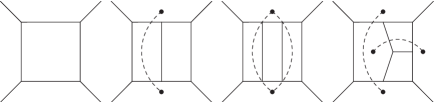
Figure 1: Dual conformally invariant diagrams through three-loops. We use the standard notation where a dotted line connecting two faces $x_{a},x_{b}$ corresponds to a numerator factor $x_{ab}$, but for clarity we omit from each diagram an overall factor of $x_{13}x_{24}$. These four diagrams correspond to the rational functions given in eqns. (3), (4), (23) and (24) respectively.

At this level of analysis we are looking simply at the naïve transformation of integrands under (26), with no consideration given to the question of infrared divergences which arise when the integral is actually performed. Following Bern:2007ct we therefore refer to any quantity invariant under (26) as pseudo-conformal. In figure 1 we review a standard diagrammatic notation for expressing the class of pseudo-conformal quantities of interest. (However at high loop-order we abandon this notation because the proliferation of numerator factors renders most diagrams illegible.) Two minor differences with respect to the standard notation are that: (1) for clarity we omit from each diagram an overall factor of $x_{13}x_{24}$ (we prove in Lemma 1 of appendix A that every four-point DCI diagram has such an overall factor); and (2) for each diagram we impose (as emphasized above) by construction that the resulting rational function of $x_{ab}$’s should have $D_{4}\times\mathfrak{s}_{L}$ symmetry and should be normalized so that the numerical factor in front of each distinct term in the sum is precisely $1$.

The translation between a diagram and its associated rational function of $x_{ab}$’s proceeds via the following simple steps. We label the four external faces $x_{1},x_{2},x_{3},x_{4}$ in cyclic order and then label the $L$ internal faces of an $L$-loop diagram as $x_{A},x_{B},\ldots$. For example, let us choose to label the fourth diagram in figure 1 as:

Each propagator bounded by faces $x_{a}$ and $x_{b}$ is associated as usual to a factor $1/x_{ab}$, while each dotted line connecting faces $x_{a}$ and $x_{b}$ is associated to a numerator factor $x_{ab}$. (Note that, as in the third diagram in figure 1, there may be $k>1$ dotted lines connecting the same two faces, in which case the numerator factor $x_{ab}$ is raised to the $k$-th power.) This diagram has 10 propagators and 2 numerator factors, so according to the rules it gives the factor

$$x_{13}x_{24}\frac{x_{24}x_{3C}}{x_{1C}x_{2A}x_{2C}x_{3A}x_{3B}x_{4B}x_{4C}x_{AB}x_{AC}x_{BC}}\,,$$ (28)

where we have restored the overall factor of $x_{13}x_{24}$ mentioned above.

The final step is to impose $D_{4}\times\mathfrak{s}_{3}$ symmetry by summing the quantity (28) over all dihedral transformations of the external $x_{1},x_{2},x_{3},x_{4}$ and all permutations of the internal $x_{A},x_{B},x_{C}$. Applying this procedure to (28), and keeping in mind our choice to normalize each distinct term with a factor of $1$, leads immediately to the expression given in (24). It is important to note that because we always impose the $D_{4}\times\mathfrak{s}_{L}$ symmetry at the level of the integrand, the choice of explicit loop momenta labeling ‘$x_{A},x_{B},\ldots$’ in these figures is largely irrelevant: they only serve as a representative with which we may present a particular numerator explicitly; any other choice would have been acceptable, as it would also generate the same rational function after symmetrization. (The labels of loop momenta with only four propagators are particularly irrelevant, as they do not appear in the numerator at all, and so are never needed to specify an explicit, representative integrand).

3.2 Dual Conformally Invariant Diagrams

It is known that there are $1,1,2,10,59$ distinct pseudo-conformal diagrams respectively at loop-orders $L=1,2,3,4,5$, respectively. However, only $1,1,2,8,34$ of those diagrams actually enter the $L$-loop four-particle integrand with nonzero coefficient; the remaining 2 four-loop and 25 five-loop diagrams do not appear in the amplitude. In Drummond:2007aua it was observed that a precise characterization can be given which distinguishes the contributing versus non-contributing diagrams: the former consist of those pseudo-conformal diagrams which are rendered infrared finite when they are evaluated off-shell, i.e. when we take the external momenta $p_{i}$ to satisfy $p_{i}^{2}\neq 0$. (Note that there are additional types of DCI diagrams one can draw when off-shell legs are allowed. These have been classified through four-loops in Nguyen:2007ya , but these additional diagrams play no role in our present analysis.)

To illustrate this point let us consider the simplest five-loop diagram which is pseudo-conformal but not DCI,

whose associated integrand is

$$\frac{x_{13}x_{24}}{x_{1E}x_{2C}x_{3D}x_{4B}x_{AB}x_{AC}x_{AD}x_{AE}x_{BD}x_{BE}x_{CD}x_{CE}}+{\rm sym.~{}(120~{}terms~{}total)}\,.$$ (29)

Let us focus on the region of integration where all four of $x_{B},x_{C},x_{D}$ and $x_{E}$ simultaneously approach $x_{A}$. Specifically let us suppose that $x_{AB},x_{AC},x_{AD},x_{AE}$ are all order ${\cal O}(\rho^{2})$ as $\rho\to 0$. In this limit there are eight vanishing propagators, giving a factor of $\rho^{16}$ in the denominator, and the integral behaves as

$$\sim\int\frac{x_{13}x_{24}}{x_{1A}x_{2A}x_{3A}x_{4A}}\frac{d^{4}x_{A}\ \rho^{15}\,d\rho}{\rho^{16}}+\cdots\,,$$ (30)

where the factor $\rho^{15}\,d\rho$ in the numerator comes from switching to radial coordinates for $x_{B},x_{C},x_{D},x_{E}$ near the point where all of these equal $x_{A}$. Evidently this integral has a divergence near $\rho=0$.

In contrast none of the diagrams shown in figure 1, nor any of the 8 (34) diagrams which are known to contribute to the 4 (5)-loop integrands, suffer from any divergences of this sort. We refer to pseudo-conformal diagrams which possess this property as genuinely dual conformally invariant (DCI) diagrams. Let us emphasize that this stands as an empirical observation, as there is no rigorous understanding of why this peculiar fact should play any important role. In particular let us emphasize that DCI diagrams most certainly do have infrared singularities when evaluated in any of the familiar regularization schemes such as dimensional regularization or the Higgs regulator of Alday:2009zm . Nevertheless, appreciating the utility of this finiteness criterion through five-loops, we adopt the conjecture that it continues to hold to all-loop order.

3.3 Classification of Four-Point DCI Diagrams Through Seven-Loops

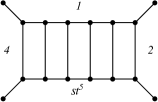
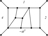
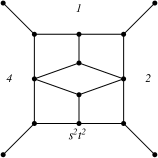
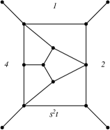
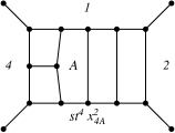
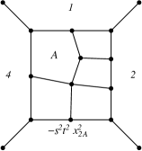
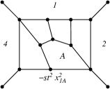
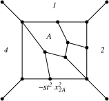
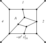
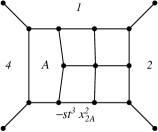
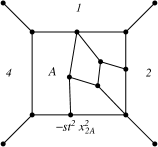
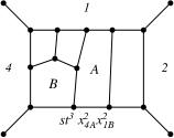
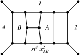
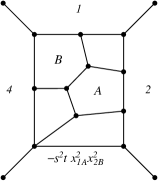
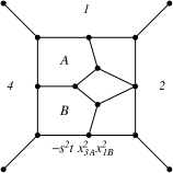
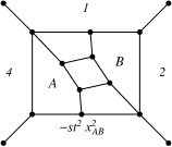
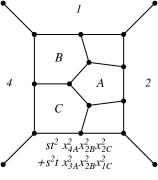
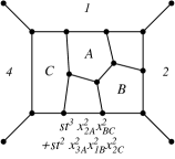
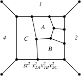
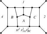
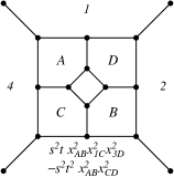
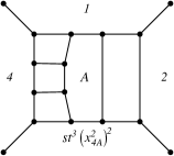
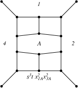
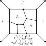
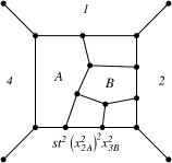
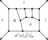
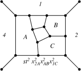
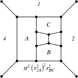
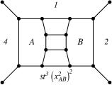
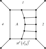
Figure 7: The integrands which generate the five-loop amplitude.

In this section we explain the steps taken to classify all DCI diagrams through seven-loops. The classification takes place in two steps: we first used an off-the-shelf program to generate all relevant distinct planar topologies, and then wrote our own code to determine, for each topology, all independent sets of numerator factors which render the diagram dual conformally invariant. The vast majority of planar graphs (in particular, any which contain a triangle— an internal face with only three edges) cannot be rendered DCI with any numerator factor, and can be rejected immediately. On the other hand, beginning at five-loops there are examples of planar graphs which are rendered dual conformally invariant by more than one inequivalent choice of numerator factor (the three occurrences of this phenomenon at five-loops are evident in fig. 7). Counting diagrams with different numerator factors separately we find $1,1,2,8,34,256,2329$ distinct four-point DCI diagrams at one- through seven-loops respectively. These come from $1,1,2,8,30,197,1489$ distinct underlying topologies (ignoring numerators). These results are summarized in table 1.

Table 1: Statistics of four-point DCI integrands through seven-loops.

Loop	# of denominator	# of distinct	# of integrands with coefficient:
	topologies	DCI integrands	$\qquad\mathbf{+1}$	$\qquad\mathbf{-1}$	$\qquad\mathbf{+2}$	$\qquad\mathbf{0}$
1	1	1	1	0	0	0
2	1	1	1	0	0	0
3	2	2	2	0	0	0
4	8	8	6	2	0	0
5	30	34	23	11	0	0
6	197	256	129	99	1	27
7	1489	2329	962	904	7	456

The first step in the classification requires the choice of a graph generating program. The popular choice qgraf Nogueira:1991ex ; qgraf , is not well-suited to the present application because of our interest exclusively in plane graphs. Note that at this point we must begin to be precise about distinguishing a ‘planar graph’, which is one that admits an embedding onto the plane with no self-intersection, from a ‘plane graph’, which is a planar graph together with a specific choice of plane-embedding. This distinction is important because a given planar graph can have more than one inequivalent embedding. Two plane graphs which correspond to the same underlying planar graph would be considered identical in scalar field theory but must be distinguished in gauge theory because they have different color index flow.

This rather subtle distinction first becomes necessary at six-loops, where we find the candidate planar graph shown in fig. 2 which admits two inequivalent plane-embeddings, only one of which can be made pseudo-conformal with a suitable numerator factor. Note that in this case the pseudo-conformal graph on the left is not DCI (it fails the finiteness criterion explained in section 3.2). We strongly suspect that it is not possible for any genuine DCI diagram to admit an inequivalent embedding in the plane, but this notion plays no role in our analysis and we only mention this phenomenon in passing as a curiosity.

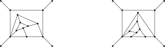
Figure 2: Two different plane embeddings of the same planar graph (they are related to each other by rotating the bottom edge of the square by 180 degrees out of the plane of the paper while leaving the other three edges fixed). The graph on the left can be made pseudo-conformal with a suitable numerator factor while the graph on the right cannot.

Returning to our main point: in order to both avoid wasting effort generating non-planar graphs in which we are not interested, and to be sure of generating all possible inequivalent plane graphs, we turn to the specialized program plantri plantripaper ; plantri which is capable of exactly what we require. The program has no concept of external lines, so to represent a four-point diagram in plantri we first ‘fold it up’ to a plane graph with $(L+4)$ faces by tying the four external lines together at a new ‘vertex at infinity.’ A given $(L+4)$-face plane graph, together with the choice of a quadrivalent vertex in the graph, may then be ‘unfolded’ to a planar four-point diagram. The process of folding and unfolding is not bijective since on the one hand two inequivalent four-point graphs may become identical when folded up, while on the other hand a given plane graph with $k>1$ quadrivalent vertices may unfold to fewer than $k$ topologically distinct four-point diagrams. The latter happens when a plane graph has a discrete symmetry which exchanges two (or more) of its quadrivalent vertices.

To generate all topologies of interest we:

1. used plantri to enumerate all plane graphs $G_{1},G_{2},\ldots$ with vertex connectivity $\geq 1$ and at least one quadrivalent vertex;

2. unfolded each graph $G_{i}$ at each of its quadrivalent vertices to obtain various four-point diagrams $G_{i}^{(1)},G_{i}^{(2)},\ldots$ (taking care to remove any duplicates, as mentioned above);

3. from the collection of diagrams so generated, we excluded any which have internal triangles, since these cannot possibly be made DCI.

It turns out that the plantri output is most naturally sorted not by $L$ but by the number of vertices in the graph. An $L$-loop DCI graph can have up to $2L+3$ vertices (including the vertex at infinity), so in order to classify all diagrams through seven-loops we need all graphs with up to 17 vertices. The reader may be interested to know that we found exactly

$$1,0,1,1,6,13,71,308,1637,8421,45229,243220,1326433$$ (31)

‘DCI candidate’ plane graphs with 5 through 17 vertices respectively. By a DCI candidate we mean a plane graph which has at least one quadrivalent vertex with the property that unfolding the graph at that point leads to a triangle-free four-point diagram for the denominator.

The four-point diagrams obtained from these DCI candidates were then fed into a custom Java program which scanned through all possible inequivalent numerator factors, selecting those which make the diagram both pseudo-conformal according to section 3.1 and finite according to the criterion reviewed in section 3.2. Many of the DCI candidates do not admit any valid numerator, while a few admit more than one inequivalent choice of numerator. The final output from our code program was a list of the $1,1,2,8,34,256,2329$ distinct DCI integrands through seven-loops advertised above; refer also to table 1.

(These numbers include 1 6-loop and 2 7-loop four-point diagrams with vertex connectivity 1, which have vertex connectivity 2 when folded up. These diagrams do not contribute to scattering amplitudes. The 6-loop example was discussed in figure 12 of Bern:2007ct .)

As part of this work we in fact generated all DCI candidate plane graphs through 18 vertices, but found it computationally prohibitive to tackle 19, which would have been necessary for a complete classification at eight-loops. While an $L$-loop DCI graph can have as many as $2L+3$ vertices, it can on the other hand have as few as $L+4$ (examples saturating this lower bound exist for $L>3$). Therefore, although our classification of DCI diagrams is complete only through seven-loops, the data we have amassed contains an enormous number of additional DCI diagrams through fourteen-loops, which we have not yet analyzed.

4 Bootstrapping the Four-Point Integrand Through Seven-Loops

The way in which the four-point multi-loop integrand can be obtained via the soft-collinear bootstrap was illustrated for the three-loop integrand in section 2.4. The condition that $(\log M_{4})^{(L)}$ has at most an $\mathcal{O}(1/\epsilon)$-pole in the soft-collinear limit (14) is equivalent to the condition that the numerator of $(\mathrm{log}~{}M_{4})^{(L)}$ (when all contributing terms are assembled over a common denominator) must vanish in this limit (as the denominator is certainly proportional to $\epsilon^{2}$). With this in mind, the procedure for obtaining the $L$-loop integrand $M_{4}^{(L)}$ from the soft-collinear bootstrap can be carried out as follows:

1. expand the log of the $L$-loop amplitude—as illustrated in eqn. (6)—and compute the contribution of each term involving strictly lower-loop amplitudes to the overall numerator in the soft-collinear limit (14); call this ‘$\mathrm{log}_{\mathrm{rest}}$’;

2. find all $L$-loop DCI integrands $I_{i}^{(L)}$ (with each one fully symmetrized with respect to permutations of the loop momentum variables $A_{1},\ldots,A_{L}$, and the $D_{4}$ dihedral symmetry of the external momenta), and compute the contribution of each to the overall numerator in the soft-collinear limit (14); call these contributions $(I_{i}^{(L)})_{\mathrm{soft}}$;

3. $\mathrm{log}_{\mathrm{rest}}$ and the $(I_{i}^{(L)})_{\rm soft}$ are of course still nontrivial polynomials in various $x_{ab}$’s, and our goal is now to determine a collection of numerical constants $c_{i}$ such that

   $$\mathrm{log}_{\mathrm{rest}}+\sum_{i}c_{i}(I_{i}^{(L)})_{\mathrm{soft}}=0.$$

   By repeatedly evaluating this equation at sufficiently many random independent values of the remaining variables ($x_{A_{2}},\ldots,x_{A_{L}}$ as well as $x_{1},\ldots,x_{4})$ this equation can be turned into a linear system on the $c_{i}$ with constant coefficients. The existence and uniqueness of the solution, which we find through seven-loops, are the central miracles of this paper.

Our conjecture is that this general strategy extends to all loop-orders. This procedure is simple enough to automate, and can be implemented efficiently enough to find all integrands through six-loops in less than 2 minutes on a sufficiently powerful computer (given knowledge of the $L$-loop DCI integrands $I_{i}^{(L)}$).

For the sake of providing a uniform reference for the reader, the results for four and five-loops are reviewed in figures 6, and 7, respectively. For six- and seven-loops, there are too many contributions to be practically included graphically here, but they may be viewed at four_point_multiloop_datafiles .

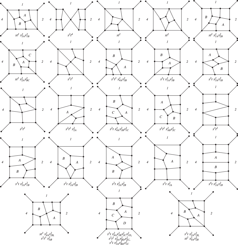
Figure 8: The 27 six-loop integrands with vanishing coefficients. Notice that each of the last three graphs admit more than one numerator; the coefficient of each possible integrand is separately zero.

Beyond five-loops, there are some interesting features worth noting, which are summarized in table 1. For example, although all 34 five-loop DCI integrands contribute to the amplitude, this is not generally the case: at six-loops, 27 of the 256 DCI integrands have vanishing coefficients; and at seven-loops, 456 of the 2329 DCI have vanishing coefficients. The 27 six-loop DCI integrands with vanishing coefficient are illustrated in figure 8.

More curiously, at six-loops there is the first appearance of a coefficient found to be ‘$+2$’; and at seven-loops, seven integrands have coefficient $+2$. These are illustrated in figures 3 and 4, respectively. It would be fascinating to see if this pattern of coefficients could be understood along the lines of the method proposed in Cachazo:2008dx .

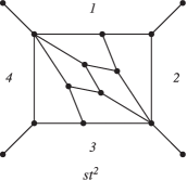
Figure 3: The only six-loop integrand contributing with coefficient $+2$.

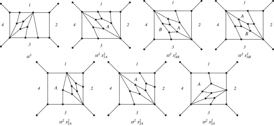
Figure 4: The 7 seven-loop contributions with coefficient $+2$.

One available and relatively simple partial check on our results involves two-particle cuts, which have been shown to iterate to all orders in SYM theory Bern:1997nh . This means that if there is an $L$-loop contribution to the integrand with the property that it can be reduced to a product of an $L-1$-loop contribution and the four-particle tree amplitude by cutting only two internal propagators, then that $L$-loop diagram must inherit the same coefficient as its $L-1$-loop ancestor. At two- and three-loops all DCI integrands have two-particle cuts; the first examples without two-particle cuts are the second and third graphs in fig. 6 (which therefore are the first graphs “allowed” by two-particle cut considerations to have coefficients other than $+1$). We have verified the consistency of our results with this principle; at seven-loops we find that 814 of the 2329 coefficients correspond to integrals which admit a two-particle cut.

Appendix A Appendix

In this appendix we collect a few useful graph theoretic results about DCI diagrams.

Lemma 1.

Every four-point DCI diagram has an overall factor of $x_{13}x_{24}$.

Proof.

We will show that the overall factor of $x_{13}x_{24}$ is required in order to pass the finiteness criterion of section 3.2. Consider an $L$-loop pseudo-conformal diagram with $P$ propagators (internal edges). By dimensional analysis there must be a total of $P-2L$ numerator factors. Now consider the behavior of the integrand in the limit when all of the $x$’s (both internal and external) approach a common point $y$. If $(x-y)^{2}=\mathcal{O}(\rho^{2})$ for all $x$’s then the integrand scales like

$$\sim\frac{\rho^{2(P-2L)}}{\rho^{2P}}\rho^{4L-1}d\rho=\frac{d\rho}{\rho}$$ (32)

where we have included the appropriate factor $\rho^{4L-1}d\rho$ from the integration measure in radial coordinates near $\rho=0$.

Of course the four $x$’s associated with the external faces are supposed to be fixed, so the fact that we have a divergence in this hypothetical limit is not yet of concern. If we remove a single external face $x_{a}$ from consideration (that is, hold $x_{a}$ fixed instead of letting it approach $y$), then the propagators adjacent to $x_{a}$ no longer contribute a factor of $\rho^{-2}$ each to eqn. (32), but the numerator factors attached to $x_{a}$ also no longer contribute a factor of $\rho^{+2}$. Since there are an equal number of each, there is no change in the conclusion and we still have a log-divergent integral.

If we remove two or more external faces from consideration this analysis is unchanged unless at some step we encounter a numerator factor $x_{ab}^{m}$ connecting two external edges. In order to avoid counting the no-longer-contributing factor of $\rho^{2m}$ twice we should multiply eqn. (32) by $\rho^{2m}$, which renders the integral finite for any $m>0$.

Therefore, by the time we’ve excluded three external faces from the limit (thereby reaching an honest limit of the integral), we must have encountered at least one numerator factor between two external faces in order to avoid a divergent integral. Since the diagram must converge for every possible limit in order to be DCI, we conclude that for any choice of three external faces $x_{a},x_{b},x_{c}$, two of them must always share a numerator factor (that is, there must be a positive power of at least one of $x_{ab}$, $x_{bc}$ or $x_{ca}$). Since $x_{ab}=0$ if $a$ and $b$ are adjacent, the only way this is possible is for the diagram to contain an overall factor of $x_{13}x_{24}$. ∎

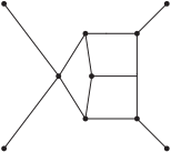
Figure 5: A degenerate graph is one in which two external legs are attached to the same vertex. Such graphs can be pseudo-conformal (although this example is not), but they cannot be DCI.

Since each of the four external faces $x_{1},\ldots,x_{4}$ appears at least once in the numerator of every DCI integrand, and conformal invariance requires that each one appears exactly as often in the denominator as in the numerator, we have the immediate

Corollary 1.

Degenerate diagrams (see figure 5) cannot be DCI.

Note Added

While we have checked our conjecture explicitly through seven loops, we are aware that starting at eight loops there are DCI integrals which do not diverge as $\mathcal{O}(1/\epsilon^{2})$ in the limit (14) and are therefore not detectable using our method. It would be interesting to see if there are further criteria that could determine the coefficients of these potential contributions to the four-particle amplitude at higher loop orders.

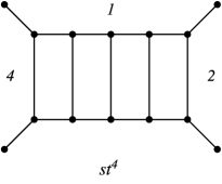
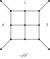
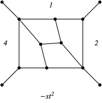
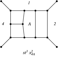
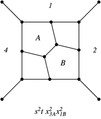
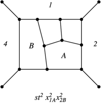
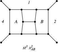
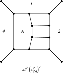
Figure 6: The integrands which generate the four-loop amplitude.

References

- (1) Z. Bern, L. J. Dixon, D. C. Dunbar, and D. A. Kosower, “Fusing Gauge Theory Tree Amplitudes into Loop Amplitudes,” Nucl. Phys. B435 (1995) 59–101, arXiv:hep-ph/9409265.
- (2) Z. Bern, L. J. Dixon, D. C. Dunbar, and D. A. Kosower, “One-Loop -Point Gauge Theory Amplitudes, Unitarity and Collinear Limits,” Nucl. Phys. B425 (1994) 217–260, arXiv:hep-ph/9403226.
- (3) Z. Bern, J. Carrasco, H. Johansson, and D. Kosower, “Maximally Supersymmetric Planar Yang-Mills Amplitudes at Five Loops,” Phys. Rev. D76 (2007) 125020, arXiv:0705.1864 [hep-th].
- (4) E. I. Buchbinder and F. Cachazo, “Two-Loop Amplitudes of Gluons and Octa-Cuts in super Yang-Mills,” JHEP 0511 (2005) 036, arXiv:hep-th/0506126.
- (5) F. Cachazo, “Sharpening The Leading Singularity,” arXiv:0803.1988 [hep-th].
- (6) F. Cachazo, M. Spradlin, and A. Volovich, “Leading Singularities of the Two-Loop Six-Particle MHV Amplitude,” Phys. Rev. D78 (2008) 105022, arXiv:0805.4832 [hep-th].
- (7) M. Spradlin, A. Volovich, and C. Wen, “Three-Loop Leading Singularities and BDS Ansatz for Five Particles,” Phys. Rev. D78 (2008) 085025, arXiv:0808.1054 [hep-th].
- (8) M. Spradlin, “Multiloop Gluon Amplitudes and AdS/CFT,” In the Proceedings of 9th Workshop on Non-Perturbative Quantum Chromodynamics, Paris, France C0706044 (2007) 05.
- (9) Z. Bern and Y.-t. Huang, “Basics of Generalized Unitarity,” J. Phys. A44 (2011) 454003, arXiv:1103.1869 [hep-th].
- (10) Z. Bern, L. J. Dixon, J. J. M. Carrasco, and H. Johansson unpublished.
- (11) S. Caron-Huot, “Loops and Trees,” JHEP 1105 (2011) 080, arXiv:1007.3224 [hep-ph].
- (12) R. H. Boels, “On BCFW Shifts of Integrands and Integrals,” JHEP 1011 (2010) 113, arXiv:1008.3101 [hep-th].
- (13) N. Arkani-Hamed, J. L. Bourjaily, F. Cachazo, S. Caron-Huot, and J. Trnka, “The All-Loop Integrand For Scattering Amplitudes in Planar SYM,” JHEP 1101 (2011) 041, arXiv:1008.2958 [hep-th].
- (14) B. Eden, G. P. Korchemsky, and E. Sokatchev, “From Correlation Functions to Scattering Amplitudes,” JHEP 1112 (2011) 002, arXiv:1007.3246 [hep-th].
- (15) L. F. Alday, B. Eden, G. P. Korchemsky, J. Maldacena, and E. Sokatchev, “From Correlation Functions to Wilson Loops,” JHEP 1109 (2011) 123, arXiv:1007.3243 [hep-th].
- (16) B. Eden, G. P. Korchemsky, and E. Sokatchev, “More on the Duality Correlators/Amplitudes,” Phys. Lett. B709 (2012) 247–253, arXiv:1009.2488 [hep-th].
- (17) B. Eden, P. Heslop, G. P. Korchemsky, and E. Sokatchev, “The Super-Correlator/Super-Amplitude Duality: Part I,” Nucl. Phys. B869 (2013) 329–377, arXiv:1103.3714 [hep-th].
- (18) B. Eden, P. Heslop, G. P. Korchemsky, and E. Sokatchev, “The Super-Correlator/Super-Amplitude Duality: Part II,” Nucl. Phys. B869 (2013) 378–416, arXiv:1103.4353 [hep-th].
- (19) B. Eden, P. Heslop, G. P. Korchemsky, and E. Sokatchev, “Hidden Symmetry of Four-Point Correlation Functions and Amplitudes in SYM,” Nucl. Phys. B862 (2012) 193–231, arXiv:1108.3557 [hep-th].
- (20) B. Eden, P. Heslop, G. P. Korchemsky, and E. Sokatchev, “Constructing the Correlation Function of Four Stress-Tensor Multiplets and the Four-Particle Amplitude in SYM,” Nucl. Phys. B862 (2012) 450–503, arXiv:1201.5329 [hep-th].
- (21) R. Akhoury, “Mass Divergences of Wide Angle Scattering Amplitudes,” Phys. Rev. D19 (1979) 1250.
- (22) A. H. Mueller, “On the Asymptotic Behavior of the Sudakov Form-factor,” Phys. Rev. D20 (1979) 2037.
- (23) J. C. Collins, “Algorithm to Compute Corrections to the Sudakov Form-Factor,” Phys. Rev. D22 (1980) 1478.
- (24) A. Sen, “Asymptotic Behavior of the Wide Angle On-Shell Quark Scattering Amplitudes in Nonabelian Gauge Theories,” Phys. Rev. D28 (1983) 860.
- (25) G. F. Sterman, “Summation of Large Corrections to Short Distance Hadronic Cross-Sections,” Nucl. Phys. B281 (1987) 310.
- (26) S. Catani and L. Trentadue, “Resummation of the QCD Perturbative Series for Hard Processes,” Nucl. Phys. B327 (1989) 323.
- (27) J. C. Collins, “Sudakov Form-Factors,” Adv. Ser. Direct. High Energy Phys. 5 (1989) 573–614, arXiv:hep-ph/0312336 [hep-ph].
- (28) L. Magnea and G. F. Sterman, “Analytic Continuation of the Sudakov Form-Factor in QCD,” Phys. Rev. D42 (1990) 4222–4227.
- (29) S. Catani and L. Trentadue, “Comment on QCD Exponentiation at Large ,” Nucl. Phys. B353 (1991) 183–186.
- (30) W. Giele and E. N. Glover, “Higher Order Corrections to Jet Cross-Sections in Annihilation,” Phys. Rev. D46 (1992) 1980–2010.
- (31) Z. Kunszt, A. Signer, and Z. Trocsanyi, “Singular Terms of Helicity Amplitudes at One-Loop in QCD and the Soft Limit of the Cross-Sections of Multiparton Processes,” Nucl. Phys. B420 (1994) 550–564, arXiv:hep-ph/9401294.
- (32) S. Catani, “The Singular Behavior of QCD Amplitudes at Two Loop Order,” Phys. Lett. B427 (1998) 161–171, arXiv:hep-ph/9802439 [hep-ph].
- (33) A. Vogt, “Next-to-Next-to-Leading Logarithmic Threshold Resummation for Deep Inelastic Scattering and the Drell-Yan Process,” Phys. Lett. B497 (2001) 228–234, arXiv:hep-ph/0010146 [hep-ph].
- (34) G. F. Sterman and M. E. Tejeda-Yeomans, “Multiloop Amplitudes and Resummation,” Phys. Lett. B552 (2003) 48–56, arXiv:hep-ph/0210130 [hep-ph].
- (35) L. F. Alday, J. M. Henn, J. Plefka, and T. Schuster, “Scattering into the Fifth Dimension of super Yang-Mills,” JHEP 1001 (2010) 077, arXiv:0908.0684 [hep-th].
- (36) J. M. Henn, S. G. Naculich, H. J. Schnitzer, and M. Spradlin, “Higgs-Regularized Three-Loop Four-Gluon Amplitude in SYM: Exponentiation and Regge Limits,” JHEP 04 (2010) 038, arXiv:1001.1358 [hep-th].
- (37) J. M. Henn, S. G. Naculich, H. J. Schnitzer, and M. Spradlin, “More Loops and Legs in Higgs-Regulated SYM Amplitudes,” JHEP 08 (2010) 002, arXiv:1004.5381 [hep-th].
- (38) Z. Bern, M. Czakon, D. Kosower, R. Roiban, and V. Smirnov, “Two-Loop Iteration of Five-Point Super-Yang-Mills Amplitudes,” Phys. Rev. Lett. 97 (2006) 181601, arXiv:hep-th/0604074 [hep-th].
- (39) F. Cachazo, M. Spradlin, and A. Volovich, “Iterative Structure within the Five-Particle Two-Loop Amplitude,” Phys. Rev. D74 (2006) 045020, arXiv:hep-th/0602228 [hep-th].
- (40) Z. Bern, M. Czakon, L. J. Dixon, D. A. Kosower, and V. A. Smirnov, “The Four-Loop Planar Amplitude and Cusp Anomalous Dimension in Maximally Supersymmetric Yang-Mills Theory,” Phys. Rev. D75 (2007) 085010, arXiv:hep-th/0610248 [hep-th].
- (41) Z. Bern et al., “The Two-Loop Six-Gluon MHV Amplitude in Maximally Supersymmetric Yang-Mills Theory,” Phys. Rev. D78 (2008) 045007, arXiv:0803.1465 [hep-th].
- (42) Z. Bern, L. J. Dixon, and V. A. Smirnov, “Iteration of Planar Amplitudes in Maximally Supersymmetric Yang-Mills Theory at Three Loops and Beyond,” Phys. Rev. D72 (2005) 085001, arXiv:hep-th/0505205.
- (43) J. M. Drummond and J. M. Henn, “Simple Loop Integrals and Amplitudes in SYM,” JHEP 1105 (2011) 105, arXiv:1008.2965 [hep-th].
- (44) N. Arkani-Hamed, J. L. Bourjaily, F. Cachazo, and J. Trnka, “Local Integrals for Planar Scattering Amplitudes,” JHEP 1206 (2012) 125, arXiv:1012.6032 [hep-th].
- (45) T. Bargheer, N. Beisert, W. Galleas, F. Loebbert, and T. McLoughlin, “Exacting Superconformal Symmetry,” JHEP 11 (2009) 056, arXiv:0905.3738 [hep-th].
- (46) J. M. Drummond, J. Henn, G. P. Korchemsky, and E. Sokatchev, “On Planar Gluon Amplitudes/Wilson Loops Duality,” Nucl. Phys. B795 (2008) 52–68, arXiv:0709.2368 [hep-th].
- (47) J. M. Drummond, J. Henn, G. P. Korchemsky, and E. Sokatchev, “Conformal Ward Identities for Wilson Loops and a Test of the Duality with Gluon Amplitudes,” Nucl. Phys. B826 (2010) 337–364, arXiv:0712.1223 [hep-th].
- (48) G. Korchemsky and A. Radyushkin, “Loop Space Formalism and Renormalization Group for the Infrared Asymptotics of QCD,” Phys. Lett. B171 (1986) 459–467.
- (49) N. Beisert, B. Eden, and M. Staudacher, “Transcendentality and Crossing,” J. Stat. Mech. 0701 (2007) P01021, arXiv:hep-th/0610251 [hep-th].
- (50) L. Mason and D. Skinner, “The Complete Planar -Matrix of SYM as a Wilson Loop in Twistor Space,” JHEP 12 (2010) 018, arXiv:1009.2225 [hep-th].
- (51) S. Caron-Huot, “Notes on the Scattering Amplitude / Wilson Loop Duality,” JHEP 1107 (2011) 058, arXiv:1010.1167 [hep-th].
- (52) A. Belitsky, G. Korchemsky, and E. Sokatchev, “Are Scattering Amplitudes Dual to Super Wilson Loops?,” Nucl. Phys. B855 (2012) 333–360, arXiv:1103.3008 [hep-th].
- (53) T. Adamo, M. Bullimore, L. Mason, and D. Skinner, “Scattering Amplitudes and Wilson Loops in Twistor Space,” J. Phys. A44 (2011) 454008, arXiv:1104.2890 [hep-th].
- (54) PDF and Mathematica files containing all our results are provided at http://goo.gl/qIKe8.
- (55) A. Hodges, “Eliminating Spurious Poles from Gauge-Theoretic Amplitudes,” arXiv:0905.1473 [hep-th].
- (56) Z. Bern, J. Carrasco, L. J. Dixon, H. Johansson, and R. Roiban, “The Complete Four-Loop Four-Point Amplitude in Super-Yang-Mills Theory,” Phys. Rev. D82 (2010) 125040, arXiv:1008.3327 [hep-th].
- (57) Z. Bern, J. Carrasco, L. Dixon, H. Johansson, and R. Roiban, “Simplifying Multiloop Integrands and Ultraviolet Divergences of Gauge Theory and Gravity Amplitudes,” Phys. Rev. D85 (2012) 105014, arXiv:1201.5366 [hep-th].
- (58) M. B. Green, J. H. Schwarz, and L. Brink, “ Yang-Mills and Supergravity as Limits of String Theories,” Nucl. Phys. B198 (1982) 474–492.
- (59) C. Anastasiou, Z. Bern, L. J. Dixon, and D. A. Kosower, “Planar Amplitudes in Maximally Supersymmetric Yang-Mills Theory,” Phys. Rev. Lett. 91 (2003) 251602, arXiv:hep-th/0309040.
- (60) J. Gluza, K. Kajda, and D. A. Kosower, “Towards a Basis for Planar Two-Loop Integrals,” Phys. Rev. D83 (2011) 045012, arXiv:1009.0472 [hep-th].
- (61) J. Drummond, J. Henn, V. Smirnov, and E. Sokatchev, “Magic Identities for Conformal Four-Point Integrals,” JHEP 0701 (2007) 064, arXiv:hep-th/0607160.
- (62) J. M. Drummond, G. P. Korchemsky, and E. Sokatchev, “Conformal Properties of Four-Gluon Planar Amplitudes and Wilson loops,” Nucl. Phys. B795 (2008) 385–408, arXiv:0707.0243 [hep-th].
- (63) D. Nguyen, M. Spradlin, and A. Volovich, “New Dual Conformally Invariant Off-Shell Integrals,” Phys. Rev. D77 (2008) 025018, arXiv:0709.4665 [hep-th].
- (64) P. Nogueira, “Automatic Feynman Graph Generation,” J. Comput. Phys. 105 (1993) 279–289.
- (65) QGRAF, http://cfif.ist.utl.pt/paulo/qgraf.html.
- (66) G. Brinkmann and B. D. McKay, “Fast Generation of Planar Graphs (expanded Version).” http://cs.anu.edu.au/bdm/papers/plantri-full.pdf.
- (67) plantri and fullgen, http://cs.anu.edu.au/bdm/plantri/.
- (68) F. Cachazo and D. Skinner, “On the Structure of Scattering Amplitudes in Super Yang-Mills and Supergravity,” arXiv:0801.4574 [hep-th].
- (69) Z. Bern, J. Rozowsky, and B. Yan, “Two-Loop Four-Gluon Amplitudes in SuperYang-Mills,” Phys. Lett. B401 (1997) 273–282, arXiv:hep-ph/9702424.