Multi-$q$ Analysis of Image Patterns

Abstract

This paper studies the use of the Tsallis Entropy versus the classic Boltzmann-Gibbs-Shannon entropy for classifying image patterns. Given a database of 40 pattern classes, the goal is to determine the class of a given image sample. Our experiments show that the Tsallis entropy encoded in a feature vector for different $q$ indices has great advantage over the Boltzmann-Gibbs-Shannon entropy for pattern classification, boosting recognition rates by a factor of 3. We discuss the reasons behind this success, shedding light on the usefulness of the Tsallis entropy.

1 Introduction

Image pattern classification is an important problem for a number of fields, e.g., for recognizing embryo development stages [1], determining protein profile from flourescence microscopy images [2], and identifying cellular structures [3]. This can be a challenging problem, specially for a large number of classes, with many different solutions proposed in the literature [4]. In this paper, however, our primary goal is to study the usefulness of the Tsallis entropy [5] by comparing it to the classic Boltzmann-Gibbs-Shannon (BGS) entropy when applied to classifying image patterns.

In statistical mechanics, the concept of entropy is related to the distribution of states, which can be characterized by the system energy levels. From an information-theoretic point of view, entropy is related to the lack of information of a system. It also represents how close a given probability distribution is to the uniform distribution, i.e., it is a measure of randomness, peaking at the uniform distribution itself. For image pattern classification, this interpretation can be useful since, for example, a symmetric, periodic or smooth image has less “possible states” than more uniformly random images. A direct link between probability distributions and such concept of entropy was proposed by Boltzmann and is the foundation of what is now known as the Boltzmann-Gibbs-Shannon (BGS) entropy. A well-know generalization of this concept, the Tsallis entropy [5], extends its application to so-called non-extensive systems using a new parameter $q$. It recovers the classic entropy for $q\to 1$, and is better suited for long-range interactions between states (e.g., in large pixel neighborhoods) and long-term memories. The Tsallis generalization of entropy has a vast spectrum of application, ranging from physics and chemistry to computer science. For instance, using the non-extensive entropy instead of the BGS entropy can produce gains in the results and efficiency of optimization algorithms [6], image segmentation [7, 8, 9] or edge detection algorithms [10].

In this paper we study the power of the Tsallis entropy in comparison to classic BGS entropy for the construction of feature vectors for classifying image patterns or textures. Given a database of patterns, typically comprising 40 classes, the goal is to determine the class of a given image sample. Our experiments show that the Tsallis entropy encoded in a feature vector for different $q$ indices produces great advantage over the Boltzmann-Gibbs-Shannon entropy for this problem, boosting recognition rates by a factor of 3.

This paper is organized as follows. A review of definitions and notation of fundamental concepts is given in Section 2. Our is described Details about the problem of image pattern classification and our approach based on the Tsallis entropy are described in Section 3. The basic experimental setup is provided in Section 4. In Section 5 experimental results towards analyzing the power of the Tsallis entropy for image pattern classification are described. Section 6 revises and concludes the paper.

2 Formulation and Notation

Assume ${p_{i}}$ is the probability distribution or the histogram of graylevels $g_{i}=1,\cdots,W$ in the grayscale image $I$, i.e., $p_{i}$ equals the number of pixels having intensity $i$ divided by the total number of pixels. We assume $g_{1}=0$ stands for black, and $g_{256}=255$ for white. The number $W$ of different graylevels is typically $256$ for 8-bit images. The BGS entropy is defined as:

$$S_{BG}=-\sum_{i=1}^{W}p_{i}\log{p_{i}},\qquad\sum p_{i}=1.$$ (1)

In the special case of a uniform distribution, $p_{i}=1/W$, so that $S_{BG}=\log W$. Similarly, the Tsallis entropy is defined as

$$S_{q}=\frac{1-\sum p_{i}^{q}}{q-1},$$ (2)

which recovers BGS entropy in the limit for $q\to 1$. The relation to BGS entropy is made clearer by rewriting this definition in the form:

$$S_{q}(p)=-\sum_{i}p_{i}^{q}\ln_{q}p_{i},$$ (3)

where

$$\ln_{q}(x)\dot{=}\frac{x^{1-q}-1}{1-q}$$ (4)

is called the $q$-logarithm, with $\ln_{q}(x)\to\ln x$ for $q\to 1$. For any value of $q>0$, $S_{q}$ satisfies similar properties to the BGS entropy; for instance, $S_{q}\geq 0$, and $S_{q}$ attains its maximum at the uniform distribution.

The BGS entropy is additive in the sense that the entropy of the whole system (the entropy of the sum) coincides with the sum of the entropies of the parts. This is not the case for the Tsallis entropy when $q\neq 1$, however. Formally,

$$S_{BG}(A+B)=S_{BG}(A)+S_{BG}(B),$$ (5)

while

$$S_{q}(A+B)=S_{q}(A)+S_{q}(B)+(1-q)S_{q}(A)S_{q}(B).$$ (6)

3 Multi-q analysis

The primary goal of image pattern classification is to assign a class label to a given image sample or window, the label being chosen among a predefined set of classes in a database. Figure 1 shows a schematic of the classification process.

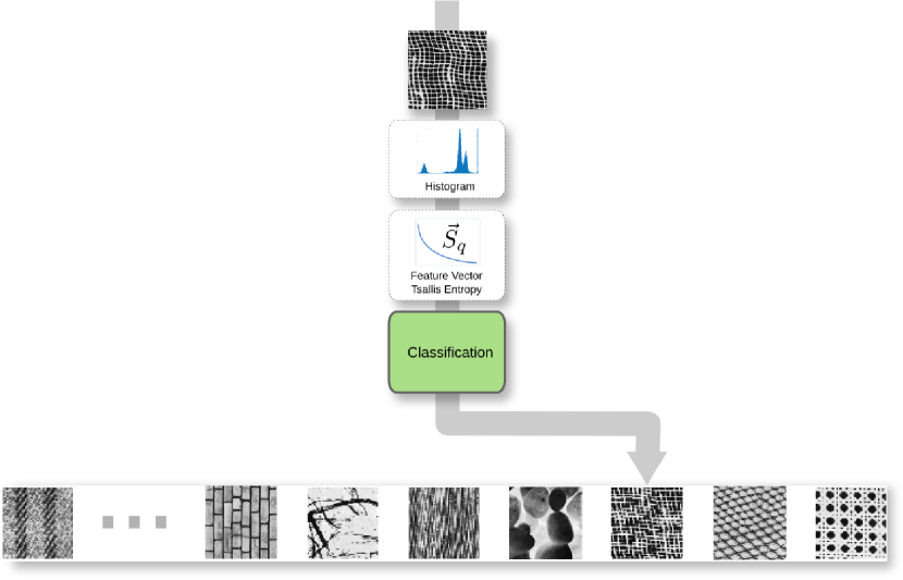
Figure 1: Our approach to image pattern classification works by extracting the histogram of an input image sample, computing a vector of Tsallis Entropies, and using that in a classifier to produce a class label among 40 classes stored in a database. The image samples in this figure are real samples illustrating the Brodatz database used in this paper.

In supervised classification, the classifier is trained from a set of samples that are known to belong to the classes (a priori knowledge). The classifier is then validated by another set of samples. This methodology can be used for pattern recognition tasks as well as for mathematical modeling. Traditionally, in image analysis, a feature vector is extracted from the image and used to train and validate the classifier. It is expected that the feature vector concentrates the most important information about the image.

In this work we investigate the Tsallis entropy as tool to analyze image information and compare it to the traditional BGS entropy. Beyond statistical mechanics, the BGS entropy is also traditionally used in information theory, and is present as a metric in many image analysis methods, for instance Gabor texture analysis, Fourier analysis, wavelet, shape analyses among many others. A classical and simple problem in image analysis is considering the distribution of pixel intensities in an image as a measure of texture, by analyzing its histogram. Such an approach has been used since the 70’s and, despite its simplicity, provides good results and is still subject of active research [11]. Therefore, we have decided to use histogram texture analysis to investigate the potentiality of Tsallis entropy applied to information theory in the context of images, and comparing its results to the those obtained with BGS entropy alone.

Histogram texture analysis begins by computing the image histogram ${p_{i}}$ of intensities, where $p_{i}$ is the number of pixels in the image for each intensity $i$. Assuming 8-bit grayscale images, it abstracts the image information into a feature vector of 256 dimensions. The histogram encodes a mixture of multiple intensity distributions representing luminosity patterns of image subsets, therefore being a clear candidate for image pattern representation for a number of classification applications. Although the histogram is largely used in image analysis, it is limited, due to its simplicity. For instance, the spatial information is not preserved by the histogram. Different images that have the same distribution of pixels have the same histogram; for instance, consider two images: a checkerboard pattern and an image split in the middle in black and white. While the visual information presented is quite different, they have the same histogram.

Despite its limitations, the image histogram has been used for different purposes, achieving good results, e.g., in image segmentation, image thresholding and pattern recognition. In this work, we are taking into account the third alternative applied to image classification. To classify an image or an image sample based on the histogram, statistical metrics are traditionally employed, such as mean, mode, kurtosis and BGS entropy. Therefore, the simplicity and popularity of the image histogram can help focus the results of the classification on the entropy analysis itself.

The concept of Tsallis entropy (and, in particular, BGS entropy) defined in Section 2 provides ways to further abstract the information of the intensity histogram. For $q=1$ we have the classic BGS entropy, strongly abstracting the 256-dimensional histogram into the extreme case of a single number $S_{1}$. This paper explores multiple $q$ parameters towards forming better feature vectors for classification. We construct feature vectors of the form $\vec{S}_{q}=(S_{q_{1}},\dots,S_{q_{n}})$, Figure 1, whose dimension $n$ (typically 4–20) provides a middle ground between the total abstraction of 1D BGS entropy and the full 256-dimensional histogram. The experiments show that very few dimensions of Tsallis-entropy values in $\vec{S}_{q}$ are already enough to outperform BGS entropy by a large factor.

4 Experimental Setup

The database used to evaluate our approach was created from Brodatz’s art book [12]. This book is a black and white photography study for art and design and it was carried out on different patterns from wood, grass, fabric, among others. The Brodatz database became popular in the imaging sciences and is widely used as a benchmark for the visual attribute of texture. The database used in our work consists of 40 classes of texture, where each class is represented by a prototypical photograph of the texture containing no other patterns. Such $512\times 512$ images are scans of glossy prints that were acquired from the author. A given image sample to be classified is much smaller than the class prototype image, $200\times 200$ in this paper. The $512\times 512$ prototype image can generate numerous $200\times 200$ image samples representing the same class using a sliding window scheme. To construct our final database we perform this sliding window process to extract 10 representative image samples for each class. Therefore, any incoming sample to be classified is of the same size as the training windows. A few samples from this database are ilustrated in Figure 1.

Several approaches for the task of classification have been proposed in the literature. Since our focus is on image representation, we used the simple and well-known Naive Bayes classifier rather than a more sophisticated classifier. Although more sophisticated classifiers have been shown to produce superior results (e.g. multilayer perceptron and support vector machine), we are interested in showing the discrimination power provided by the features themselves rather than showing the classification power of classifiers.

In order to objectively evaluate the performance of the Tsallis entropy versus BGS entropy for classification, we use the stratified 10-fold cross-validation scheme [13]. In this scheme, the samples are randomly divided into 10 folds, considering that each fold contains the same proportions of the classes (i.e. for the Brodatz dataset, each fold contains 40 samples, one sample of each class). At each run of this scheme, the classifier is trained using all but one fold and then evaluated on how it classifies the samples from the separated fold. This process is repeated such that each fold is used once as validation. The performance is averaged, generating a single number for classification rate which represents the overall proportion of success over all runs. A standard deviation is also computed and displayed when significant. In the next section, moreover, a confusion matrix is eventually generated to analyze the performance of a specific classifier strategy. The confusion matrix is very well known in statistical classification and artificial intelligence. It is an $n\times n$ matrix where $n$ is the number of classes, and whose entry $(i,j)$ expresses how many patterns of class $i$ were labeled as class $j$. It allows analyzing the error of the classification and which class was most wrongly classified.

5 Experimental Results

We have conducted two sets of experiments to evaluate the texture recognition performance. The aim of the first set of experiments is to analyze the power of the Tsallis entropy with only one $q$ value and compare its performance against that of the BGS entropy. The second set of experiments is devised to analyze the Tsallis entropy with a multi-$q$ approach, including analysis of different sets of $q$’s.

5.1 Classification Results: single $q$

To fairly compare the BGS and Tsallis entropies, we conducted an experiment using a single value of $q$, that is, the feature vector reduced to a single number for the purpose of our study. Note, however, that in a practical system one would use a higher-dimensional feature vector (i.e., more numbers) to represent an image sample. In the Brodatz dataset, using the BGS entropy alone yielded a classification rate of $25\%(\pm 5.78)$. To compare it to the Tsallis entropy, we need to choose an appropriate value of $q$. The classification rate of different values of $q$ are presented in the plot of the Figure 2. The best result of $32.75\%(\pm 6.17)$ was obtained by the Tsallis entropy with $q=0.2$. Notice that any Tsallis entropy with $q<1$ outperforms the BGS entropy. Moreover, note that in the most cases, the classification rate decreases as the value of $q$ increases.

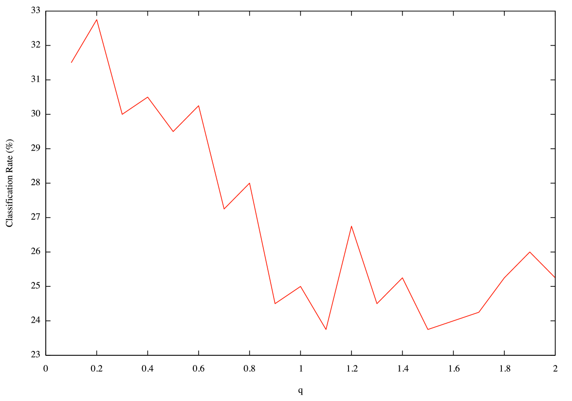
Figure 2: Classification rate using a single value of $q$ at a time.

We expected that for texture images in general (i.e., beyond Brodatz) the highest classification rates are also obtained for values of $q$ close to $0.2$. Table 1 presents the best values of $q$ for different texture image datasets, including CUReT [14] (Columbia-Utrecht Reflectance and Texture Database), Outex from the University of Oulu [15], and VisTex from MIT. For all but the VisTex dataset the best value of $q$ was $0.2$. For VisTex the highest classification rate of $21.30\%(\pm 3.27)$ was obtained by $q=0.1$ while $q=0.2$ achieved a correct classification rate of $20.72\%(\pm 3.21)$. Moreover, the Tsallis entropy using $q=0.2$ outperforms the BGS entropy for all datasets. Note that these results concern the effectiveness of a single number to abstract the information of an image window. We strees that on a practical system one would likely represent a $200\times 200$ image with a larger set of numbers (features).

Dataset	best q	Classification Rate	BGS Entropy
Brodatz	0.2	$32.75\%(\pm 6.17)$	$25.00\%(\pm 5.78)$
VisTex	0.1	$21.30\%(\pm 3.27)$	$16.90\%(\pm 3.26)$
CUReT	0.2	$10.14\%(\pm 0.84)$	$08.64\%(\pm 0.77)$
Outex	0.2	$14.19\%(\pm 2.37)$	$13.38\%(\pm 2.03)$

Table 1: Classification results for different texture image datasets and the best value of $q$. The Tsallis entropy outperforms the BGS entropy for all datasets.

5.2 Classification Results: multiple $q$

One hypothesis for the power of the Tsallis entropy concerning pattern recognition is that each $S_{q}$ could hold different information about the pattern. Therefore, different values of $q$ used together could improve classification rates. Indeed, Figure 3 shows that the $S_{q}$ curve can help in distinguishing the patterns – the feature vector $\vec{S}_{q}=(S_{0.1},S_{0.2}...,S_{2})$ is plotted for three different textures, giving an idea of the discriminating power of the Tsallis entropy.

Since the nature of the $S_{q}$ curve is exponential, it is difficult to grasp the differences between the patterns. In order to improve the visualization of pattern behavior through the $S_{q}$ curve, we calculated the mean vector $\vec{\mu}$, that is, the average $S_{q}$ curve of the 400 samples of the image database, and plotted the difference of $\vec{S_{q}}$ and $\vec{\mu}$ for 10 patterns picked at random, Figure 4. Notice that the first values of $q$ present the best pattern discrimination, which agrees with the results of the experiments for a single $q$, where a $q$ around $0.2$ performs best.

Figure 3: The feature vector $(S_{0.1},...,S_{2})$ for three different textures, giving an idea of the discriminating power of the Tsallis entropy.

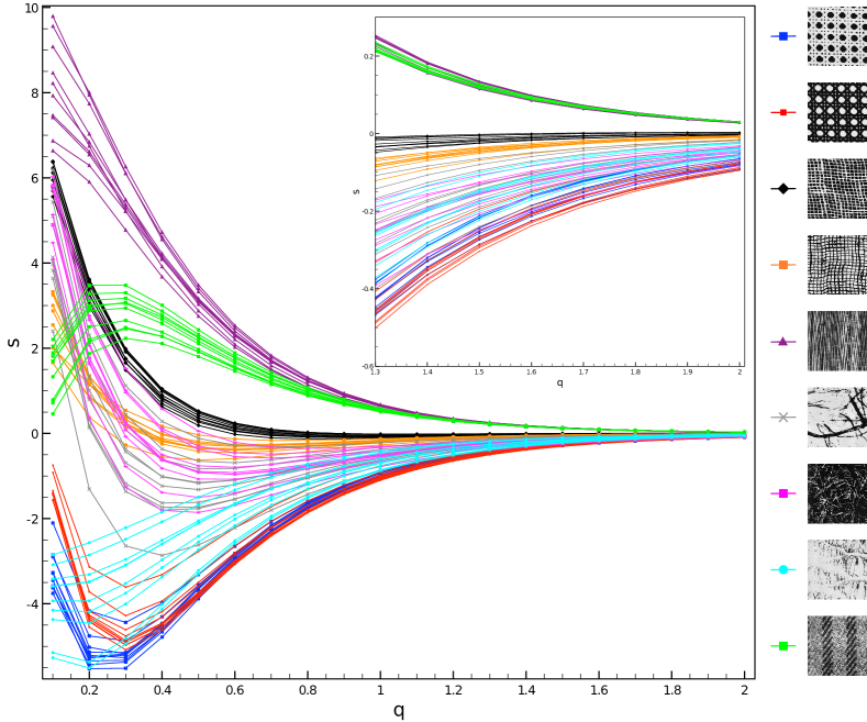
Figure 4: Tsallis entropy versus $q$ for different patterns. Each color and symbol combination represents a class of texture pattern.

To use Tsallis entropy curve as a pattern recognition tool, we composed a feature vector $\vec{S_{q}}$ in the interval q=0.1:0.1:2 (i.e., $q$ from 0.1 to 2 in increments of 0.1). Using this feature vector of 20 elements, a classification rate of $73.75\%(\pm 6.49)$ was achieved. We also constructed feature vectors using different intervals of values of $q$. The classification results are shown in Table 2. These results corroborate the hypothesis that a multi-q approach can improve the power of the Tsallis entropy applied to pattern recognition. The multi-q strategy using only 20 elements results in a gain of $41\%$ compared to best value of $q$ and a gain of $48.75\%$ compared to the BGS entropy.

Range of $q$	#Features	Classification Rate %
0.2	1	$32.75(\pm 6.17)$
0.5:0.5:2	5	$52.75(\pm 6.27)$
0.2:0.2:2	10	$67.00(\pm 6.43)$
0.1:0.1:2	20	$73.75(\pm 6.21)$
0.05:0.05:2	40	$75.75(\pm 6.54)$
0.01:0.01:2	200	$77.25(\pm 6.49)$
0.005:0.005:2	400	$77.50(\pm 6.01)$
0.001:0.001:2	2000	$78.50(\pm 6.16)$

Table 2: Classification results for different sets of $q$.

To visualize the behavior of the texture classes, we use a Karhunen-Loeve transform (or principal components analysis, PCA). This allows us to projecting the feature vectors onto a lower-dimensional space which is easier to visualize, and where the variance is higher as possible. The PCA was applied to the feature vectors of the 400 samples (40 classes) of the Brodatz dataset and a scatter plot was obtained, Figure 5. As we can see, the classes become organized in distinguished cluster, illustrating the power of classification of the multi-q approach.

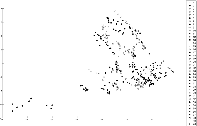
Figure 5: To give a visual idea of the discriminating power of the Tsallis entropy, a principal components analysis (PCA) was performed on Brodatz’s 40 classes considering a 20-dimensional feature vector $(S_{0.1},...,S_{2})$, and visualized as a 2-dimensional scatter plot of the first two principal components.

5.3 Feature selection: enhancing the discriminanting power of the $S_{q}$ curve

We have noticed that composing a feature vector with different $S_{q}$’s can boost the discriminative power of the Tsallis entropy. Nevertheless, the feature vector was composed by $q$ in the range $0.1,0.2,\dots 2$ and, as remarked in Figure 2, there are $q$ values in the interval that do not achieve the maximum classification. Therefore, a question arises: is the information of the entire interval $0<q\leq 2$ aiding to distinguish the image patterns?

Feature selection is a technique used in multivariate statistics and in pattern recognition that selects a subset of relevant features with the aim of improving the classification rate and also its robustness. There are several algorithms for feature selection, the reader can find a feature selection survey in [16]. We have used a very simple strategy in the present work to clarify the influence of the different $q$ in the classification process. The main idea is use only the $S_{q}$ values that presents significant contribution to the classification rate. Figure 6(a) plots the classification rate using the first $S_{q}$’s, taking different quantities of these; e.g., for the first datapoint of the curve a single $S_{q}$ was used, $(S_{0.1})$, in the second datapoint two $S_{q}$’s, $(S_{0.1},S_{0.2})$, and at position $n$ on the $x$ axis, $n$ $S_{q}$’s. The curve shows there are values of $S_{q}$ that improve the classification rate but there are also values of $q$ that do not increase the classification rate or even decrease it. To make the contribution of each $S_{q}$ easier to see, we take the derivative of the curve of the Figure 6(a), shown in the Figure 6(b). We performed feature selection by picking the $q$’s whose values in the derivative curve are greater than $t$.

(a)(b)

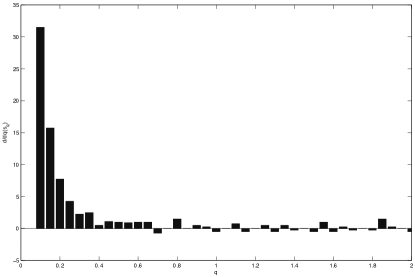
Figure 6: (a) Classification rate for feature vectors using the first $S_{q}$ elements: for a value of $q$, the curve gives the classification when using $\vec{S}_{q}=(S_{0.1},\dots,S_{q})$ as a feature vector. The number of elements in the feature vector increases for each element of x axis. (b) the derivative of the previous curve.

The feature selection reduces the number of features and increases the classification power of the multiple $q$ entropy approach. The Table 3 shows results of the feature selection over multi-$q$ approach for different range of $q$ at the interval 0 to 2. As can be observed with just 4 elements the result is equivalent to a feature vector with size 20 without the feature selection (see Table 2) and with 27 elements, the feature selection approach overcome the performance of a 2000 size feature vector (Table 2). The results demonstrates the feature selection algorithm presents a optimal performance of the mult-$q$ approach. The main reason of the performance increase is that the algorithm can select the $S_{q}$ significant elements.

The confusion matrices for different representative approaches to entropy-based image classification investigated in this paper are shown in 3D Figure LABEL:fig:feature:selection1. An arbitrary entry $(x,y)$ of a confusion matrix expresses how many patterns of class $x$ were labeled as class $y$, and this is visualized as height $z$ in the figure. This visualizations gives insight into the error of the classification and which class was most wrongly classified.

Range of $q$	#Features	Classification Rate %
0.5:0.5:2	4	52.75
0.2:0.2:2	4	73.75
0.1:0.1:2	6	80
0.05:0.05:2	7	80.25
0.01:0.01:2	21	81.5
0.005:0.005:2	26	81.75
0.001:0.001:2	27	82

Table 3: Classification results for feature selection from different step sizes of $q$

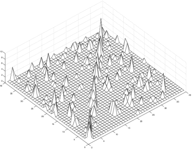
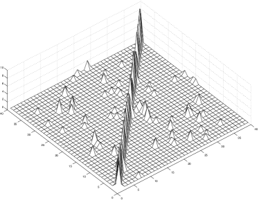
(a)(b)
(c)(d)

Figure 7: Confusion matrices for (a) BGS entropy alone, (b) Tsallis entropy with $q=0.2$, (c) multi-$q$ approach using the feature vector $\vec{S}_{q}=(S_{0.1},\dots,S_{2})$, and (d) feature vector constructed with the feature selection technique described in the paper.

6 Conclusion

In this paper we showed how the Tsallis entropy can be used in image pattern classification with great advantage over the classic entropy. The parametrized Tsallis entropy enables larger-dimensional feature vectors using different values of $q$, which yields vastly better performance than using BGS entropy alone. This points to the fact that the Tsallis entropy for different $q$ does encode much more information from a given histogram than the BGS entropy. In fact, one of the results show that as little as 4 values of $q$, together, are enough to outperform the BGS entropy by about $3\times$. Work to further analyze the implications of these results within a deeper information-theoretic framework is underway, shedding light into the usefullness of the Tsallis entropy for general problems of pattern recognition.

References

- [1] H. Zhong, W.-B. Chen, C. Zhang, Classifying fruit fly early embryonic developmental stage based on embryo in situ hybridization images, in: Proceedings of the 2009 IEEE International Conference on Semantic Computing, ICSC ’09, IEEE Computer Society, Washington, DC, USA, 2009, pp. 145–152.
- [2] H. Janssens, D. Kosman, C. Vanario-Alonso, J. Jaeger, M. Samsonova, J. Reinitz, A high-throughput method for quantifying gene expression data from early drosophila embryos, Development Genes and Evolution 215 (7) (2005) 374–381.
- [3] J. Böhm, A. Frangakis, R. Hegerl, S. Nickell, D. Typke, W. Baumeister, Toward detecting and identifying macromolecules in a cellular context: template matching applied to electron tomograms, Proceedings of the National Academy of Sciences 97 (26) (2000) 14245.
- [4] R. Duda, P. Hart, D. e. a. Stork, Pattern classification, Vol. 2, Wiley New York, 2001.
- [5] C. Tsallis, Introduction to Nonextensive Statistical Mechanics: Approaching a Complex World, Springer, 2009.
- [6] C. Tsallis, D. Stariolo, Generalized simulated annealing, Physica A: Statistical and Theoretical Physics 233 (1-2) (1996) 395–406.
- [7] C. Chang, Y. Du, J. Wang, S. Guo, P. Thouin, Survey and comparative analysis of entropy and relative entropy thresholding techniques, in: IEE Proceedings of Vision, Image and Signal Processing, Vol. 153, IET, 2006, pp. 837–850.
- [8] M. de Albuquerque, I. Esquef, A. Mello, M. de Albuquerque, Image thresholding using tsallis entropy, Pattern Recognition Letters 25 (9) (2004) 1059–1065.
- [9] P. Rodrigues, G. Giraldi, Computing the q-index for tsallis nonextensive image segmentation, in: XXII Brazilian Symposium on Computer Graphics and Image Processing, IEEE, 2009, pp. 232–237.
- [10] A. Hamza, Nonextensive information-theoretic measure for image edge detection, Journal of Electronic Imaging 15 (2006) 013011.
- [11] A. Barbieri, G. de Arruda, F. Rodrigues, O. Bruno, L. Costa, An entropy-based approach to automatic image segmentation of satellite images, Physica A: Statistical Mechanics and its Applications 390 (3) (2011) 512–518.
- [12] P. Brodatz, Textures: a photographic album for artists and designers, Dover Publications ^ eNew York New York, 1966.
- [13] I. Witten, E. Frank, M. Hall, Data mining: Practical machine learning tools and techniques, 3rd Edition, Morgan Kaufmann, 2011.
- [14] K. Dana, B. Van-Ginneken, S. Nayar, J. Koenderink, Reflectance and Texture of Real World Surfaces, ACM Transactions on Graphics (TOG) 18 (1) (1999) 1–34.
- [15] O. T., M. T., P. M., V. J., K. J, H. S., Outex - new framework for empirical evaluation of texture analysis algorithms., 2002, proc. 16th International Conference on Pattern Recognition, Quebec, Canada, 1:701 - 706.
- [16] L. Molina, L. Belanche, À. Nebot, Feature selection algorithms: A survey and experimental evaluation, in: Data Mining, 2002. ICDM 2002. Proceedings. 2002 IEEE International Conference on, IEEE, 2002, pp. 306–313.