Reduced density matrix and entanglement entropy of permutationally invariant quantum many-body systems

Abstract

In this paper we discuss the properties of the reduced density matrix of quantum many body systems with permutational symmetry and present basic quantification of the entanglement in terms of the von Neumann (VNE), Renyi and Tsallis entropies. In particular, we show, on the specific example of the spin $1/2$ Heisenberg model, how the RDM acquires a block diagonal form with respect to the quantum number $k$ fixing the polarization in the subsystem conservation of $S_{z}$ and with respect to the irreducible representations of the $\mathbf{S_{n}}$ group. Analytical expression for the RDM elements and for the RDM spectrum are derived for states of arbitrary permutational symmetry and for arbitrary polarizations. The temperature dependence and scaling of the VNE across a finite temperature phase transition is discussed and the RDM moments and the Rényi and Tsallis entropies calculated both for symmetric ground states of the Heisenberg chain and for maximally mixed states.

I Introduction

Entanglement properties of interacting quantum many-body systems Amico-Review lies at the heart of many quantum information processes such as measurement based quantum computation, teleportation, security of quantum key distribution protocols, super-dense coding, etc. Nielsen . Being a principal resource for quantum information, one is interested to know how much entanglement is present in a system and how much of it can be used or created. Entanglement also provides benchmarks for success of quantum experiments. Entanglement properties are presently investigated for several spin chains Vidal , Latorre , Jin-Korepin , Korepin , Peschel2004 , Peschel2005 , Its , Entanglement_Heisenberg , PSS , for strongly correlated fermions Korepin , Gu , Anfossi and pairing models Zanardi , for itinerant bosons Helmerson , etc.

The calculation of the entanglement involves the knowledge of the reduced density matrix (RDM) characterizing quantum systems in contact with the environment such as a thermal bath or a larger system of which the original system is a subsystem. In particular, the spectrum of the RDM, which by definition is real and nonnegative with all eigenvalues summing up to one, provides an intrinsic characterization of a subsystem. The relative importance of a subsystem state, indeed, is directly related to the weight that the corresponding eigenvalue has in the RDM spectrum. Thus, for instance, the fact that the eigenvalues $\lambda_{i}$ of the RDM for a one dimensional quantum interacting subsystems decay exponentially with $i$ implies that the properties of the subsystems are determined by only a few states. This property is crucial for the success of the density-matrix renormalization group (DMRG) method White92 in one dimension. In two dimensions this property is lost PeschelChung and the DMRG method fails.

For a subsystem consisting of $n$ sites (or $n$ q-bits) the RDM is of rank $2^{n}$ so that for large $n$ the calculation of the spectrum becomes a problem of exponential difficulty. While the spectrum of the full RDM for subsystems with a small number of sites (e.g. $n\leq 6$) has been calculated NienhuisCalabrese2009 , the full RDM for arbitrary $n$ is, to our knowledge, exactly known only for the very special case of non interacting quantum systems such as free fermions (see e.g. PeschelFreeFermionRDM ) or free bosons.

The aim of the present paper is to analytically calculate the elements of the RDM of permutational invariant quantum systems of arbitrary size $L$, for arbitrary permutational symmetry of the state of the system (labelled by an integer number $0<r<L/2$) and arbitrary sizes $n$ (number of q-bits) of the subsystem. We remark that the invariance under the permutational group physically implies that the interactions among sites have infinite range. As an example of such system we consider the Heisenberg model of spin $1/2$ on a full graph consisting of $L$ sites, with fixed value of spin polarization $S_{z}=L/2-N$. For this system we calculate the RDM and the entanglement von Neumann entropy (VNE) for a subsystem of arbitrary $n\geq 1$    sites for arbitrary $L,N.$ The temperature dependence and the scaling properties of the VNE across a finite temperature phase transition occurring in the system are also discussed, and the RDM moments and the Rényi and Tsallis entropies calculated both for symmetric ground states of the Heisenberg chain and for maximally mixed states.

The plan of the paper is the following. In Section I we discuss model equations and provide basic definitions. In Section II we consider the main properties of RDM elements and show how the symmetry properties of the system allow to decompose the RDM into a block diagonal form. In Sec. IV we present an exact analytical expression of the RDM matrix elements for arbitrary parameters values whose rigorous proof is provided in the thermodynamic limit in the appendix B and for the case of fully symmetric states in the appendix A. In Sec. V we provide an analytical characterization of the RDM spectrum and discuss scaling properties and temperature dependence of the von Neumann entropy. In Sec. VI, moments of the reduced density matrix are discussed and several quantities of interest like mutual information, Renyi and Tsallis entropies, are calculated. In the last section the main results of the paper are briefly summarized.

II Model equation and basic definitions

We consider a permutational invariant system of $L$ spins $1/2$ on a complete graph with fixed total spin polarization $S_{z}=L/2-N$ and described by the Hamiltonian

$$H=-\frac{J}{2L}\left(\mathbf{S}^{2}-\frac{L}{2}\left(\frac{L}{2}+1\right)\right)+hS_{z}$$ (1)

Here $\mathbf{S}\equiv(S_{x},S_{y},S_{z}),\;S_{\alpha}=\frac{1}{2}\sum_{i=1}^{L}\sigma_{i}^{\alpha}$, with $\sigma_{i}^{\alpha}$ Pauli matrices acting on the factorized $\prod\limits_{1}^{L}\otimes C_{2}$ space. This Hamiltonian is invariant under the action of the symmetric group $\mathbf{S}_{L}$ Sagan and conserves $S_{z}$, $[H,S_{z}]=0$. A complete set of eigenstates of $H$ are states $|\Psi_{L,N,r}\rangle$ associated to filled Young tableaux (YT) of type $\{L-r,r\}_{(N)}$ (see Mario94 for details), where the subscript $N$ denotes the number of quanta present in the tableau and the symbol $\{L-r,r\}$ refers to a tableau of only two rows, with $L-r$ boxes (sites) in the first row and $r$ in the second row. For the Hamiltonian in (1) we have:

$$H|\Psi_{L,N,r}\rangle=E_{L,N,r}|\Psi_{L,N,r}\rangle,$$

$$E_{L,N,r}=\frac{1}{2}\left(\frac{Jr}{L}(L-r+1)+h(L-2N)\right),$$ (2)

$$S_{z}|\Psi_{L,N,r}\rangle=\left(\frac{L}{2}-N\right)|\Psi_{L,N,r}\rangle$$

where $N=0,1,...,L$ determines possible values of the spin polarization and $r$ takes values $r=0,1,...,\max(N,L-N)$. Notice that, due to the symmetry and antisymmetry of a YT with respect to rows and columns, respectively, the state $|\Psi_{L,N,r}\rangle$ can exist only if $N\geq r$ (for the explicit form of the state $|\Psi_{L,N,r}\rangle$ see Eq. (55) below). The degeneracies of the eigenvalues $E_{L,N,r}$ are given by the dimension of the corresponding YTs:

$$\deg_{L,r}=\binom{L}{r}-\binom{L}{r-1}.$$ (3)

Consider a set of vectors $|\Psi_{u}\rangle$, $u=1,...\deg_{L,r}$, forming an orthonormal basis in the eigenspace of $H$ with eigenvalue $E_{L,N,r}$. We define the density matrix of the whole system as

$$\sigma_{L,N,r}=\frac{1}{\deg_{L,r}}\sum_{u=1}^{\deg_{L,r}}|\Psi_{u}\rangle\langle\Psi_{u}|.$$ (4)

It can be easily shown that $\sigma_{L,N,r}$ possess the following properties:

$\mathbf{i)}$ The matrix $\sigma_{L,N,r}$ has eigenvalues $\lambda_{1}=\lambda_{2}=...=\lambda_{\deg_{L,r}}=(\deg_{L,r})^{-1}$, with remaining $2^{L}-\deg_{L,r}$ eigenvalues all equal to zero. This follows from the fact that each vector $|\Psi_{u}\rangle$ is an eigenvector of $\sigma_{L,N,r}$ with eigenvalue $\frac{1}{\deg_{L,r}}$. Since the spectrum of $\sigma_{L,N,r}$ is real and nonnegative with all eigenvalues summing up to $1$, the remaining $2^{L}-\deg_{L,r}$ eigenvalues must vanish.

$\mathbf{ii)}$ Matrix $\sigma_{L,N,r}$ satisfies: $(\sigma_{L,N,r})^{2}=\frac{1}{\deg_{L,r}}\sigma_{L,N,r}$. This follows from the definition (4) and the orthonormality condition $\langle\Psi_{w}|\Psi_{u}\rangle=\delta_{uw}$.

$\mathbf{iii)}$ Matrices $\sigma_{L,N,r}$ commute with each other $[\sigma_{L,N,r}\,,\,\sigma_{L,N^{\prime},r^{\prime}}]=0$. This follows from orthogonality of eigenspaces of $H$ for different eigenvalues.

$\mathbf{iv)}$Introducing the operator $P_{ij}$, permuting subspaces $i$ and $j$ of the Hilbert space $\prod\limits_{1}^{L}\otimes C_{2}$ on which the matrix $\sigma_{L,N,r}$ acts, we have that: $[\sigma,P_{ij}]=0$ for any $i,j$.

This last property can be proved by considering

$$P_{ij}\sigma_{L,N,r}P_{ij} =\frac{1}{\deg_{L,r}}\sum_{u=1}^{\deg_{L,r}}P_{ij}|\Psi_{u}\rangle\langle\Psi_{u}|P_{ij}$$

$$=\frac{1}{\deg_{L,r}}\sum_{u=1}^{\deg_{L,r}}|\Psi_{u}^{\prime}\rangle\langle\Psi_{u}^{\prime}|.$$ (5)

The vectors $|\Psi_{u}^{\prime}\rangle=P_{ij}|\Psi_{u}\rangle$ form an orthonormal basis, being $\langle\Psi_{w}^{\prime}|\Psi_{u}^{\prime}\rangle=\langle\Psi_{w}|P_{ij}^{T}P_{ij}|\Psi_{u}\rangle=\langle\Psi_{w}|\Psi_{u}\rangle=\delta_{uw}$, because $P_{ij}^{T}=P_{ij}$, and $(P_{ij})^{2}=I$. Now, the sum $\sum_{u=1}^{\deg_{L,r}}|\Psi_{u}\rangle\langle\Psi_{u}|=I_{\deg_{L,r}}$ is a unity operator in a factor space of dimension $\deg_{L,r}$, and therefore it does not depend on the choice of the basis. Note that vector $|\Psi_{u}^{\prime}\rangle$ belongs to the same factor space as $|\Psi_{u}\rangle$, because permutation $P_{ij}$ only results in different enumeration. Consequently,

$$P_{ij}\sigma P_{ij}=\rho\text{, \ \ \ or \ }[\sigma,P_{ij}]=0.$$ (6)

The latter property implies that in Eq. (4) the sum over the orthogonalized set of basis vector in (4) can be replaced by the symmetrization of the density matrix directly, namely $\sigma_{L,N,r}=\frac{1}{L!}\sum_{P}|\Psi_{12...L}\rangle\langle\Psi_{12...L}|$, where the sum is over all $L!$ permutations of indexes $1,2,...L$, and $|\Psi_{12...L}\rangle$ is some unit eigenvector of $H$ with eigenvalue $E_{L,N,r}$. In particular, it is convenient to choose $|\Psi_{12...L}\rangle\equiv|\Psi_{L,N,r}\rangle$,

$$\sigma_{L,N,r}=\frac{1}{L!}\sum_{P}|\Psi_{L,N,r}\rangle\langle\Psi_{L,N,r}|.$$ (7)

It is evident that such a sum is invariant with respect to permutations and that $\sigma_{L,N,r}$ is properly normalized: $Tr\sigma_{L,N,r}=1$.

The Reduced Density Matrix (RDM) of a subsystem of $n$ sites is defined by tracing out $L-n$ degrees of freedom from the density matrix of the whole system:

$$\rho_{(n)}=Tr_{L-n}\sigma_{L,N,r}.$$ (8)

Due to the properties (6) and (8), $\rho_{(n)}$ does not depend on the particular choice of the $n$ sites, and satisfies the property (6) in its subspace (we omit the explicit dependence of $\rho_{(n)}$ on $L,N,r$ for brevity of notations).

III RDM properties and block diagonal form

The RDM can be calculated in the natural basis by using its definition in terms of observables: $\langle\hat{f}\rangle=Tr(\rho_{(n)}\hat{f})$ where $\hat{f}$ is a physical operator acting on the Hilbert space of the $2^{n}\times 2^{n}$ subsystem. The knowledge of the full set of observables determines the RDM uniquely. Indeed, if we introduce the natural basis in the Hilbert space of the subsystem, $\prod\limits_{k=1}^{n}\otimes C_{2}$, the elements of the RDM in this basis are

$$\rho_{j_{1}j_{2}...j_{n}}^{i_{1}i_{2}...i_{n}}=\left\langle\hat{e}_{j_{1}j_{2}...j_{n}}^{i_{1}i_{2}...i_{n}}\right\rangle=Tr\left(\rho_{(n)}\hat{e}_{j_{1}j_{2}...j_{n}}^{i_{1}i_{2}...i_{n}}\right),$$ (9)

with $\hat{e}_{j_{1}j_{2}...j_{n}}^{i_{1}i_{2}...i_{n}}=\prod\limits_{k=1}^{n}\otimes\hat{e}_{j_{k}}^{i_{k}}$ and $\hat{e}_{j}^{i}$ a $2\times 2$ matrix with elements $\left(\hat{e}_{j}^{i}\right)_{kl}=\delta_{ik}\delta_{jl}$. The matrix $\hat{e}_{j_{1}j_{2}...j_{n}}^{i_{1}i_{2}...i_{n}}$ has only one nonzero element, equal to $1$, at the crossing of the row $2^{n-1}i_{1}+2^{n-2}i_{2}+...+i_{n}+1$ and the column $2^{n-1}j_{1}+2^{n-2}j_{2}+...+j_{n}+1$ (all indices $i,j$ take binary values $i_{k}=0,1$ and $j_{k}=0,1$). To determine all the RDM elements one must find a complete set of observables and compute the averages $\left\langle\hat{e}_{j_{1}j_{2}...j_{n}}^{i_{1}i_{2}...i_{n}}\right\rangle$. Note that a generic property of the RDM elements, which follows directly from (6), is that any permutation between pairs of indices $(i_{m},j_{m})$ and $(i_{k},j_{k})$ does not change its value, e.g.

$$\rho_{j_{1}j_{2}...j_{n}}^{i_{1}i_{2}...i_{n}}=\rho_{j_{2}j_{1}...j_{n}}^{i_{2}i_{1}...i_{n}}=\rho_{j_{n}j_{1}...j_{2}}^{i_{n}i_{1}...i_{2}}=...=\rho_{j_{n}j_{n-1}...j_{1}}^{i_{n}i_{n-1}...i_{1}}.$$ (10)

Another property of the RDM follows from the $S_{z}$ invariance

$$\rho_{j_{1}j_{2}...j_{n}}^{i_{1}i_{2}...i_{n}}=0,\text{\qquad if }i_{1}+i_{2}+...+i_{n}\neq j_{1}+j_{2}+...+j_{n}.$$ (11)

Thus, for instance, the RDM for $n=2$ has only $6$ nonzero ($4$ different) elements , $\rho_{00}^{00},\rho_{01}^{10}=\rho_{10}^{01},$ $\rho_{10}^{10}=\rho_{01}^{01}$ and $\rho_{11}^{11}$, subject to normalization $Tr\rho_{(2)}=\rho_{00}^{00}+$ $\rho_{10}^{10}+\rho_{01}^{01}+\rho_{11}^{11}=1$. It is convenient to introduce the operators

$$\hat{e}_{0}^{1}=\begin{pmatrix}0&0\\ 1&0\end{pmatrix}\equiv\sigma^{-},\;\;\;\;\;\hat{e}_{1}^{0}=\begin{pmatrix}0&1\\ 0&0\end{pmatrix}\equiv\sigma^{+},$$

$$\hat{e}_{0}^{0}=\begin{pmatrix}1&0\\ 0&0\end{pmatrix}\equiv\hat{p}\;,\;\;\;\;\;\hat{e}_{1}^{1}=\begin{pmatrix}0&0\\ 0&1\end{pmatrix}\equiv\hat{h}\;.$$

If we represent a site spin up with the vector $\binom{1}{0}$ and a site spin down with the vector $\binom{0}{1}$ then $\hat{p}_{k}$ and $\hat{h}_{k}$ are spin up and spin down number operators on site $k$, while $\sigma^{-},\sigma^{+}$ represent spin lowering and rising operators, respectively. Thus, for instance, the observable $\langle\hat{p}_{1}\hat{p}_{2}\hat{h}_{3}\hat{h}_{4}...\hat{h}_{n}\rangle=$ $\rho_{0011...1}^{0011...1}$ gives the probability to find spins down at sites $3,4,...n$, and spins up at sites $1,2$, while the observable $\langle\sigma_{1}^{+}\sigma_{2}^{+}\sigma_{3}^{-}\sigma_{4}^{-}\hat{h}_{5}...\hat{h}_{n}\rangle=\rho_{11001...1}^{00111...1}$ gives the probability to find spins down at sites $5,6,...n$, spin lowering at sites $3,4$ and spin rising at sites $1,2$. Note that the latter operator conserves the total spin polarization since the number of lowering and rising operators is the same. Also note that the correlation functions with a non conserved polarization vanish, e.g.

$$\langle\sigma_{1}^{+}\sigma_{2}^{+}\sigma_{3}^{-}\hat{h}_{4}\hat{h}_{5}...\hat{h}_{n}\rangle=\rho_{11011...1}^{00111...1}=0,$$ (12)

in accordance with (11).

One can take advantage of the $S_{z}$ invariance (e.g. Eq. 11) to block diagonalize the RDM into independent blocks $B_{k}$ of fixed polarization $k=i_{1}+i_{2}+...+i_{n}=j_{1}+j_{2}+...+j_{n}$ (here $k=0,...,n$ gives the number of spin up present in the subsystem). In Fig. 1 the blocks $B_{k}$ appearing in the RDM $\rho_{(5)}$ have been shown for the case $n=5,L=18,N=8,r=6$. We remark that the $n+1$ diagonal blocks correspond to the values $s_{z}=(n-2k)/2$, $k=0,1,...,n$ the subsystem polarization can assume, being the block decomposition a direct consequence of the $S_{z}$ symmetry. The dimension of the block $B_{k}$ coincides therefore with the number of possible configurations that $k$ spin up can assume on $n$ sites, e.g. $\dim B_{k}=\binom{n}{k}$. One can check that the sum of the dimensions of all blocks gives the full RDM dimension, i.e. $\sum_{k}\dim B_{k}=2^{n}$. Notice that the block diagonal form in the natural basis is achieved only after a number of permutations of rows and columns of the RDM have been performed. We also remark that the fact that the middle block $B_{3}$ in Fig. 1 has all vanishing anti-diagonal elements is purely accidental (see also remark at the end of Sec.II).

Blocks $B_{k}$ consist of elements $e_{j_{1}}^{i_{1}}\otimes e_{j_{2}}^{i_{2}}\otimes e_{j_{3}}^{i_{3}}\otimes...\otimes e_{j_{n}}^{i_{n}}$  of the original matrix, with $\sum\limits_{1}^{n}i_{p}=\sum\limits_{1}^{n}j_{p}=k$ and $i_{p}=0,1$, $j_{p}=0,1$. In its turn, all elements $e_{j_{1}}^{i_{1}}\otimes e_{j_{2}}^{i_{2}}\otimes e_{j_{3}}^{i_{3}}\otimes...\otimes e_{j_{n}}^{i_{n}}$ of the block $B_{k}$ can be further block diagonalized (see below). In the natural basis, this diagonalization is done according to the number of pairs of type $(e_{1}^{0}\otimes e_{0}^{1})$ present in the elements. In the following we denote by $G_{Z}$ the part of the block associated to elements with $Z$ pairs $(e_{1}^{0}\otimes e_{0}^{1})$ in it. The sub-block $G_{0}$ of the block $B_{k}$ is formed by the elements containing $k$ terms $e_{1}^{1}$ and ($n-k$) terms $e_{0}^{0}$ in the product, i.e. $e_{1}^{1}\otimes...e_{1}^{1}\otimes e_{0}^{0}\otimes...\otimes e_{0}^{0}$ and all permutations. All such elements lie on the diagonal, and vice versa, each diagonal element of $B_{k}$ belongs to $G_{0}$. Consequently, the sub-block $G_{0}$ consists of $\binom{n}{k}$ elements. The number of elements, $\deg G_{1}(k)$, in the sub-block $G_{1}$ is equal to the number of elements of the type $e_{1}^{0}\otimes e_{0}^{1}\otimes e_{i_{1}}^{i_{1}}\otimes e_{i_{2}}^{i_{2}}\otimes...\otimes e_{i_{n-2}}^{i_{n-2}}$, such that $1+0+i_{1}+i_{2}+...+i_{n-2}=k$.

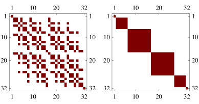
Figure 1: Left panel. RDM $\rho_{(5)}$ in the natural basis. Parameters are $L=18,N=8,r=6$. Black boxes denote non zero elements. Right panel. The same matrix of the left panel after the following chain of permutations of rows and columns have been applied to it: $R_{8,14}R_{14,18}R_{8,21}R_{3,29}R_{2,28}R_{6,16}R_{4,9}$. ($R_{i,j}$ denote the operator which exchange first columns $i$ and $j$ and then rows $i$ and $j$). Black boxes denote non zero elements. Block diagonal structure associated with values of $k=0,1,...,5$ is evident. The single element present in blocks $k=0,5,$ are $1/34$ and $1/153$, respectively. Elements values inside other k-blocks are given in Fig. 2.

Using elementary combinatorics we obtain:

$$\deg G_{1}(k)=\binom{2}{1}\binom{n}{2}\binom{n-2}{k-1}.$$ (13)

Analogous calculations for arbitrary sub-block $G_{Z}$ yields

$$\deg G_{Z}(k)=\binom{2Z}{Z}\binom{n}{2Z}\binom{n-2Z}{k-Z}.$$ (14)

From the restriction $\sum_{1}^{n}i_{p}=\sum_{1}^{n}j_{p}=k$ we deduce that the block $B_{k}$ contains non-empty parts $G_{0},G_{1},...,G_{\min(k,n-k)}$, leading to the following decomposition:

$$B_{k}=\bigcup\limits_{Z=0}^{\min(k,n-k)}G_{Z}.$$ (15)

Indeed, the normalization condition following from (15), gives

$$\sum_{Z=0}^{\min(k,n-k)}\deg G_{Z}(k)=\binom{n}{k}^{2}.$$ (16)

It is important to note that all elements of $G_{Z}$ are equal. This is a direct consequence of the property in Eq. (10). A graphical representation of the $B_{k}$ block for a particular choice of $L,N,r$, is given in Fig.2.

It is instructive to discuss the structure of blocks $B_{k}$ in terms of the matrices $\sigma$ in in (7) since this structure is directly connected with the block diagonalization of the RDM with respect the the irreps of $S_{n}$.

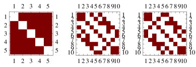
Figure 2: Blocks $B_{k}$ for $k=1,4$ (left panel), $k=2$ (central panel) and $k=3$ (right panel) corresponding to the block diagonal form of $\rho(5)$ in Fig.1. In the left panel white and black boxes denote elements $5/306$ and $1/2448$ for $k=1$ and elements $2/51$ and $1/1020$ for case $k=4$. In the center panel white boxes denote the element $1/1020$ while black boxes, except for the ones along the diagonal which are all equal to $2/51$, denote the element $-1/1190$. In the right panel white boxes denote the element $1/1360$ while black boxes denote the element $-3/4760$, except the ones along the diagonal which are equal to $1/34$. The matrices $\sigma_{n,k,s}$ involved in the decomposition in (III) have the same shapes as blocks $B_{k}$ in the left panel for $\sigma_{511}=\sigma_{541}$, with white and black boxes denoting elements $1/5$ and $-1/20$, respectively. The shape of matrix $\sigma_{521}$ (resp. $\sigma_{522}$) is the same as in the central panel, with white boxes denoting $1/60$ (resp. $-1/30$ ) and black ones $-1/15$ (resp. $1/30$ ), except the ones along the diagonal which are $1/10$, and shape of $\sigma_{531}$ (resp. $\sigma_{532}$) is the shape is as in right panel with white box denoting $1/60$ (resp. $-1/30$) and black ones $-1/15$ (resp. $1/30$ ) except for the ones along the diagonal which are given by $1/10$. The $5\times 5$matrices $\sigma_{510}=\sigma_{540}$, and $10\times 10$ matrices $\sigma_{520}=\sigma_{530}$ have all elements equal to $1/5$ and $1/10$, respectively, while $\sigma_{500}=\sigma_{550}=1$.

We have, indeed, that each block $B_{k}$ can be decomposed in the form

$$B_{k}=\sum\limits_{s=0}^{\min(k,n-k)}\alpha_{n,k,s}^{L,N,r}\sigma_{n,k,s}$$ (17)

where $\sigma_{n,k,s}$ are associated to filled YTs of type $\{n-s,s\}_{(k)}$ and $\alpha_{n,k,s}^{L,N,r}$ are coefficients related to the corresponding eigenvalues $\lambda_{n,k,s}^{L,N,r}$ of the RDM by

$$\alpha_{n,k,s}^{L,N,r}=\lambda_{n,k,s}^{L,N,r}\deg_{n,s}.$$ (18)

Notice that the matrices $\sigma_{n,k,s}$ in the natural basis have dimension $2^{n}$ and coincide with the ones given in (4) . In the proper basis (e.g. that of the irrep of $S_{n}$) they have dimension $\deg_{n,s}\times\deg_{n,s}$ and contribute to $B_{k}$ with a sub-block of dimension $\deg_{n,s}$ corresponding to the filled YT of type $\{n-s,s\}_{(k)}$. In performing this reduction one actually achieves the diagonalization of the block $B_{k}$, as it is evident from (17) (recall that $\sigma_{n,k,s}$ have eigenvalues $1/\deg_{n,s}$). A first reduction of the matrices is achieved by accounting for the $S_{z}$ symmetry discussed before, this leading to matrices $\sigma_{n,k,s}$ of size $\binom{n}{k}\times\binom{n}{k}$. In Fig. 2 are also given the matrices $\sigma_{n,k,s}$ appearing in the decomposition of blocks $B_{k}$ for the specific example considered in Fig. 1 and for $k=0,...5,\;s=0,1,2$. One can check that these matrices satisfy all properties of matrix $\sigma$ given above and in particular, the number of their nonzero eigenvalues (all equal to $1/\deg_{n,s}$) coincides with the dimension $\deg_{n,s}$ of the YT to which they are associated. This implies that they can be further reduced from $\binom{n}{k}\times\binom{n}{k}$ to $\deg_{n,s}\times\deg_{n,s}$ size by eliminating the spurious $\binom{n}{k}-\deg_{n,s}$ zero eigenvalues (these eigenvalues arise because in the natural basis the dimension of the representation is larger than the one of the $S_{n}$ irreps). This is achieved by using the singular valued decomposition of the matrix $\sigma$ to write it in the form: $\sigma=UWV^{T}$, where $W$ a diagonal matrix whose elements are the singular values and $U$ and $V$ are orthogonal matrices: $U^{T}U=V^{T}V=1$, with superscript $T$ denoting the transpose (this decomposition can be obtained very efficiently numerically numrecepies ).

The reduction to the sub-blocks of $B_{k}$ in the proper $S_{n}$ representation is then achieved as: $\sigma=uwv^{T}$ where $u$ and $v$ are rectangular matrices of dimension $\binom{n}{k}\times\deg_{n,s}$ obtained from $U$ and $V$ by omitting the columns corresponding to the zero eigenvalues and the matrix w is a $\deg_{n,s}\times\deg_{n,s}$ diagonal matrix with the nonzero eigenvalues along the diagonal (in our case, since the nonzero eigenvalues of $\sigma$ are all equal to 1, $w$ reduces to an unit matrix). The matrix $w$ then provides the representation of $\sigma_{n,k,s}$ in the proper $S_{n}$ space leading to the full diagonalization of the block $B_{k}$.

Thus, for example, the block diagonal form of the RDM in the right panels of Fig. 1 (see also Fig.2) is expressed in terms of matrices $\sigma$ as

$$B_{1} =\lambda_{510}\sigma_{510}\oplus 4\lambda_{511}=\lambda_{540}\sigma_{540}\oplus 4\;\lambda_{541}\sigma_{541}=B_{4},$$

$$B_{2} =\lambda_{520}\,\sigma_{520}\oplus 4\;\lambda_{521}\,\sigma_{521}\oplus 5\;\times\lambda_{522}\,\sigma_{522},$$ (19)

$$B_{3} =\lambda_{530}\,\sigma_{530}\oplus 4\;\lambda_{531}\,\sigma_{531}\oplus 5\;\times\lambda_{532}\,\sigma_{532},$$

with blocks $B_{0}=\lambda_{500}=\frac{1}{34}$, $B_{5}=\lambda_{550}=\frac{1}{153}$ and eigenvalues $\lambda_{510}=11/612$, $\lambda_{520}=76/1785$, $\lambda_{530}=19/595$, $\lambda_{540}=11/255$, of degeneracy $1$, eigenvalues $\lambda_{511}=13/816$, $\lambda_{521}=299/7140$, $\lambda_{531}=299/9520$, $\lambda_{541}=13/340$, of degeneracy $4$, and eigenvalues $\lambda_{522}=13/357$, $\lambda_{532}=13/476$, of degeneracy $5$ (having adopted the short notation $\lambda_{nks}\equiv\lambda^{L,N,r}_{n,k,s}$, the chosen parameters $L=18,N=8,r=6$ are understood).

IV Analytical expression of RDM elements

The main analytical property of the RDM is summarized in the following statement:

Elements $g_{Z}$ of a sub-block $G_{Z}$ of a block $B_{k}$ of the RDM (8), for arbitrary $L,N,r,n$, are given by:

$$g_{Z}=\frac{\binom{L-n}{N-k}}{\binom{L}{N}\binom{N}{Z}\binom{L-N}{Z}}\sum_{m=0}^{Z}\left(-1\right)^{m}\binom{N-r}{Z-m}\binom{L-N-r}{Z-m}\binom{r}{m}.$$ (21)

This expression has been derived by extrapolating exact results obtained for finite size calculations using symbolic programs and its correctness has been checked by comparing with brute force numerical calculation of the RDM up to large sizes. Notice that Eq. (21) completely defines all elements of the RDM in the natural basis. In practice, to find the element $P,Q$ of the RDM $\left(\rho_{(n)}\right)_{PQ}$ in the natural basis one must take the binary representation of numbers $P-1$ and $Q-1$ (which provide the sets of integers $\{i_{p}\}$ and $\{j_{p}\}$, respectively), find the corresponding number $Z$ and use (21).

A proof of the statement for arbitrary $L,N,n$ is given in Appendix A for the specific case $r=0$ corresponding to fully symmetric states. A proof of Eq. (21) which is valid in the thermodynamical limit $L\rightarrow\infty$ is provided in Appendix B. In this respect, we remark that in the limit $L\rightarrow\infty$ Eq. (21) simplifies to

$$g_{Z}=p^{n-k}(1-p)^{k}\eta^{Z},$$ (22)

where we denote with $p=\frac{N}{L}$, $\mu=\frac{r}{L}$ and

$$\eta=\frac{(p-\mu)(1-p-\mu)}{p(1-p)}.$$ (23)

For a proof of Eq (22) see Appendix B.

V Spectral properties of RDM and entanglement entropy

The existence of two representations for the block $B_{k}$ of the RDM, one in terms of matrices $G_{Z}$ given in Eq. (15), the other involving matrices $\sigma_{n,k,s}$ and given in Eq. (17), have been shown in Sec.II. These representations, together with the invariance of $G_{Z}$ and $\sigma_{n,k,s}$ with respect to permutations, imply the existence of linear relations of the form

$$\hat{G}_{Z}(k)=\sum_{s=0}^{\min(k,n-k)}\beta_{Z}(k,s)\sigma_{n,k,s}$$ (24)

where $\beta_{Z}(k,s)$ are constants and $\hat{G}_{Z}$ denotes the matrix formed by all elements of $G_{Z}$. Since $\sigma_{n,k,s}$ commute for different $s$ (see the property $(\mathbf{iii)}$ of matrices $\sigma$ in Sec. I), we have that also $\hat{G}_{Z}$ commute

$$[\hat{G}_{Z}(k),\hat{G}_{Z^{\prime}}(k)]=0.$$ (25)

This also implies that all RDM eigenvalues $\lambda_{n,k,s}^{L,N,r}$ must be linear combinations of elements $g_{Z}$ of matrices $G_{Z}$. One can show, indeed, that the general expression of the RDM eigenvalues is

$$\lambda_{n,k,s}^{L,N,r}=\sum_{Z=0}^{\min(k,n-k)}\alpha_{Z}^{(s)}(n,k)g_{Z},$$ (26)

with coefficients $\alpha_{Z}^{(s)}(n,k)$ given by

$$\alpha_{Z}^{(s)}(n,k)=(-1)^{Z}\sum_{i=0}^{k-s}(-1)^{i}\binom{k-s}{i}\binom{n-k+s}{i}\binom{s}{Z-i},$$ (27)

where $Z,s=0,1,...,k$. From Eq. (27) one can see that $\alpha_{Z}^{(s)}(n,k)$ are integer coefficients which, due to the property (25), do not depend on the characteristics of the original state $L,N$ and $r$. Thus the dependence of the RDM eigenvalues on these parameters enters only through the elements $g_{Z}$ (21). Moreover, one can shown that they satisfy the following relations

$$\alpha_{0}^{(s)}(n,k)=1,$$ (28)

$$\sum_{Z=0}^{\min(k,n-k)}\alpha_{Z}^{(0)}(n,k)=\binom{n}{k},$$ (29)

$$\sum_{Z=0}^{\min(k,n-k)}\alpha_{Z}^{(s)}(n,k)=0\;\quad\text{for }s>0,$$ (30)

$$\sum_{Z=0}^{\min(k,n-k)}\alpha_{Z}^{(s)}(n,k)\binom{Z}{p}=0,\;p=0,1,...s-1,$$ (31)

$$\sum_{Z=0}^{\min(k,n-k)}\alpha_{Z}^{(s)}(n,k)\binom{Z}{k}=\alpha_{k}^{(s)}(n,k)=(-1)^{s}\binom{n-k-s}{k-s}.$$ (32)

a proof of which can be found for special cases in acta .

From Eqs. (21), (22), (26), (27), the explicit analytical form of the complete spectrum of the RDM is obtained.

The knowledge of the RDM spectrum allows to investigate the bipartite entanglement, e.g. the entanglement of a subsystem of size $n$ with respect to the rest of the system (see Amico-Review for a review). This is done in terms of the entanglement entropy which for pure states at zero temperature coincides with the non Neumann entropy

$$S_{(n)}=-tr(\rho_{(n)}\log_{2}\rho_{(n)})=-\sum\lambda_{k}\log_{2}\lambda_{k},$$ (33)

where $\lambda_{k}$ the eigenvalues of the RDM $\rho_{(n)}$, obtained from the density matrix $\rho$ of the whole system as $\rho_{(n)}=tr_{(L-n)}\rho$. For the infinite range ferromagnetic Heisenberg model at zero temperature the density matrix of the whole system is a projector on the symmetric ground state $\rho=|\Psi(L,N)\rangle\langle\Psi(L,N)|$ considered in Entanglement_Heisenberg where it was shown that $\lambda_{k}=(_{k}^{n})(_{N-k}^{L-n})/(_{N}^{L})$, where $k=0,1,...\min(n,N)$. In the limit of large $n$ the VNE becomes

$$S_{(n)}\approx\frac{1}{2}\log_{2}(2\pi epq)+\frac{1}{2}\log_{2}\frac{n(L-n)}{L}.$$ (34)

One can show that a zero temperature (e.g. $\mu=r/L=0$) Entanglement_Heisenberg the spectrum of the reduced density matrix is described by a binomial distribution $\lambda_{k}=p^{k}q^{n-k}\binom{n}{k}$ which converges to a Gaussian for large $n$

$$\lambda_{k}\approx\frac{1}{\sqrt{2\pi\sigma^{2}}}\exp\left(-\frac{n^{2}(p-\frac{k}{n})^{2}}{2\sigma^{2}}\right),$$ (35)

where $\sigma^{2}=np(1-p)\gg 1$.

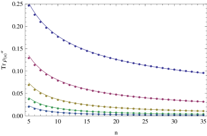
Figure 3: Traces of the powers $\alpha=2,2.5,3,3.5,4$ (from top to bottom, respectively) of the RDM versus the block size $n$ for symmetric states $r=0$, as obtained from the analytical expression (47) for $p=0.5$ (continuous curves) and from exact expressions of RDM eigenvalues (26), (27) (full dots) for $L=2\,*10^{3}$.

For finite temperature one introduces the thermal VNE for a block of size $n$ as

$$S_{(n)}(\beta)=-tr(\tilde{\rho}_{(n)}\left(\beta\right)\log_{2}\tilde{\rho}_{(n)}\left(\beta\right)),$$ (36)

$$\tilde{\rho}_{(n)}\left(\beta\right)=\frac{1}{\mathcal{Z}}\sum_{r}d_{r}e^{-\beta E_{r}}\langle\rho_{(n)}(r)\rangle,$$ (37)

where $\tilde{\rho}_{(n)}(\beta)$ is the thermal reduced density matrix, $\mathcal{Z}$ is the partition function, and $\langle.\rangle$ denotes the equal weight (thermic) average over all orthogonal degenerate states, corresponding to a given permutational symmetry. Note that $\langle\rho_{(n)}(r)\rangle$ commutes with any permutation operator and does not depend on the choice of sites in the block but only on its size $n$. Also note that the matrices $\langle\rho_{(n)}(r)\rangle$ commute for different $r$

$$\left[\langle\rho_{(n)}(r)\rangle,\langle\rho_{(n)}(r^{\prime})\rangle\right]=0,$$ (38)

so that the diagonalization of $\tilde{\rho}_{(n)}(\beta)$ is reduced to the diagonalization of $\langle\rho_{(n)}(r)\rangle$ for arbitrary $r$. From Eq. (37) the computation of the temperature-dependent von Neumann entropy is easily made with the help of the general expression of the eigenvalues of the RDM in Eq.s (26),(27) for states of arbitrary permutational symmetry. While $p=N/L$ is the system polarization, the relation between the temperature $T$ and the parameter $\mu=r/L$ is fixed by the condition of the minimum of the free energy of the whole system defined by the spectrum (2) and its degeneracy. It has the form (see EntanglementThermic , Entanglement_Theorems )

$$\frac{J}{2T}=\frac{1}{(1-2\mu)}\ln\left(\frac{1-\mu}{\mu}\right).$$ (39)

The scaling of the thermal VNE across a phase transition, which occurs in the system with infinite range interactions at finite temperature $T_{c}\neq 0$ Mario94 , has been considered in Ref. EntanglementThermic , Entanglement_Theorems . In this case it was shown that the VNE of a block od size $n$ scales as

$$S_{(n)}=\left\{\begin{array}[c]{cc}\frac{1}{2}\log n+\frac{1}{2}\log 2\pi epq&\text{for }T=0\\ nH(\mu)+\frac{1}{2}\log n+C(p,\mu)&\text{ \ \ \ \ \ \ \ for }0<T<T_{c}\\ nH(\min(p,1-p))&\text{ for }T\geq T_{c}\end{array}\right.$$ (40)

where $H(a)=-a\log a-(1-a)\log(1-a)$, $q=1-p$ and $C(p,\mu)$ does not depend on $n$.

Figure 4: Rényi entropies for symmetric ground states of the Heisenberg chain versus polarization $p=N/L$ for the cases $\alpha=1,2,3,4,6,8$ (curves from top to bottom, respectively) and for $n=20$. Continuous curves refer to the analytical expression in (49) while the full dots are obtained from exact calculations using RDM eigenvalues in (26) (27) for $L=2\,*10^{3}$ and same polarization.

Another quantity of interest strictly related to the entanglement entropy is the mutual information, $I_{AB}$, which measures the work necessary to erase all correlations in the bipartite system Amico-Review :

$$I_{AB}=S(A)+S(B)-S(AB),$$ (41)

where $S(X)$ is the VNE of the subsystem $X$. At nonzero temperature we find for a subsystem of size $n$ of a system with size $L$, using (40):

$$I_{AB}(n,L,T)=\frac{1}{2}\log(n(L-n))+Const$$ (42)

for all $T<T_{c}$ and $I_{AB}(T)=0$ for $T\geq T_{c}$.

VI Moments of the reduced density matrix and Rényi and Tsallis entropies

Besides the entanglement entropy, the Rényi, $R(\alpha)$, renyi and Tsallis, ($T(\alpha)$, tsallis entropies, defined as

$$S_{R}(\alpha,n)=\frac{\log Tr(\rho_{(n)}^{\alpha})}{1-\alpha},\;\;S_{T}(\alpha,n)=\frac{Tr(\rho_{(n)}^{\alpha})-1}{1-\alpha},$$ (43)

with $\alpha$ a positive real number, are also commonly used as a measure of entanglement. Notice that both expressions reduce the VNE in the limit $\alpha\rightarrow 1$. The knowledge of these generalized entropies requires the computation of $Tr(\rho_{(n)}^{\alpha}$ which, except special cases (see below) it is a very difficult task. For $\alpha$ positive integers, however, the moments $Tr(\rho_{(n)}^{\alpha}$ can be computed using a quantum field theory (QFT) procedure which is known as the replica method replica (reminiscent of the ”replica trick” of disordered systems).

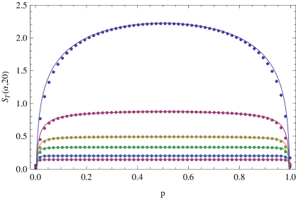
Figure 5: Same as in Fig. 4 but for Tsallis entropy. Continuous curves refer to the analytical expression in (50) while the full dots are obtained from exact calculations using RDM eigenvalues.

In this case the entanglement entropy is obtained through an analytical continuation of $Tr(\rho_{(n)}^{\alpha})$ from positive integers to real $\alpha$ values, using

$$S_{(}n)=-lim_{\alpha\rightarrow 1}\frac{\partial}{\partial\alpha}Tr[{\rho_{(n)}}^{\alpha}].$$ (44)

In the case of 1+1 conformal field theories critical models at zero temperature (for ground state) the displays universal properties, namely

$$Tr(\rho_{(n)}^{\alpha})=C_{\alpha}\left(\frac{L}{\pi}\sin\frac{\pi n}{L}\right)^{-c\frac{\alpha-1/\alpha}{6}}$$ (45)

where $c$ is the central charge of the underlying conformal field theory. Similarly, for the quantum XY chain with periodic boundary conditions at zero temperature it has been shown that the RDM is independent on the block size n and the moments can be expressed in the form franchini

$$(\frac{1}{2}Tr(\rho_{(n)}^{\alpha}))^{1/2}=\frac{\prod_{m=1}^{\infty}(1+e^{-2m\epsilon\alpha})}{\prod_{m=1}^{\infty}(1+e^{-2m\epsilon})^{\alpha}}$$ (46)

where $\epsilon$ depends on the anisotropy and transverse field parameters. Except these and few other cases, analytical properties of RDM for interacting systems are largely unexplored. The characterization of the RDM spectrum given for permutational invariant systems allows to provide another exact result for the RDM moments which is not accessible by QFT methods (our model is not conformal invariant).

In particular, the ground states of the ferromagnetic Heisenberg chain being characterized by the YT with $r=0$, are fully symmetric states with respect to the permutations (see appendix). For these states then one can obtain the analytical expression of $Tr(\rho^{\alpha})$ straightforwardly, using the Gaussian distribution of the symmetric RDM eigenvalues derived in (35). The approximation $\sum_{k}...\approx n\int...dx$, indeed, readily provides

$$Tr(\rho^{\alpha}) \approx n\int_{-infty}^{infty}\frac{1}{(2\pi\sigma^{2})^{\alpha/2}}\exp\left(-\frac{n^{2}(p-x)^{2}}{2\sigma^{2}}\alpha\right)dx=$$

$$=\frac{1}{\sqrt{\alpha}}\left(2\pi pq\right)^{\frac{1-\alpha}{2}}n^{\frac{1-\alpha}{2}}$$ (47)

In Fig. 3 we compare the behavior of the traces of the RDM powers with the block size $n$, as obtained from Eq. (47) and from exact expressions of RDM eigenvalues. We see that the agreement is very good this confirming the correctness of our analytical derivation.

In the case the original global state has the form of a maximally mixed state, i.e. is the sum of equally weighted projectors on symmetric states $|\Psi_{L,N}\rangle$ of the form $\rho=\frac{1}{L+1}\sum_{N=0}^{L}|\Psi_{L,N}\rangle\langle\Psi_{L,N}|$, the reduced density matrix has one eigenvalue only $\lambda_{k}=\frac{1}{n+1}$, which is degenerate $n+1$ times. In this case, then

$$Tr(\rho_{(n)}^{\alpha})=(n+1)^{1-\alpha}.$$ (48)

Notice that the entanglement entropy at $T=0$ in (40) follows from (47) using the expression (44) of the QFT replica method. Another quantity directly related to the RDM moments is the effective dimension defined as $d_{eff}=\frac{1}{Tr(\rho_{(n)}^{2})}$. Summarizing the above results, we have for this quantity that:

$$d_{eff}=\left\{\begin{array}[c]{c}\sim n\text{ for maximally mixed symmetric state}\\ \sim\sqrt{n}\text{ for pure symmetric state}\\ \sim n^{1/4}\text{ for critical XXZ\ model ground state}\\ \sim n^{c/4}\text{ for a critical state with central charge }c\text{ }\end{array}\right.$$

From the expression of $Tr(\rho_{(n)}^{\alpha})$ in 47 the Rényi and Tsallis entropies for fully symmetric states follow as

$$S_{R}(\alpha,n) =\frac{1}{2}\log(2\pi npq)-\frac{\log\alpha}{2(1-\alpha)},$$ (49)

$$S_{T}(\alpha,n) =\frac{1}{\sqrt{\alpha}}\frac{(2\pi npq)^{\frac{1-\alpha}{2}}-1}{1-\alpha}.$$ (50)

In Figs. 4, 5, we compare the above analytical expressions for the Rényi and Tsallis entropies with exact calculations using the RDM eigenvalues in Eqs (26) (27), from which we see that a very good agreement is found. Also notice that in the limit $\alpha=1$ both entropies reduce to the entanglement entropy (40) at $T=0$: $S_{R}(1,n)=S_{T}(1,n)=\frac{1}{2}\log 2\pi epqn$.

In general, for arbitrary permutational symmetries and for finite temperatures, one must recourse to direct calculations using the general expression (26) for the RDM eigenvalues, since it is not easy in these cases to give simple analytical expressions of $\alpha$. The study of the analytical properties of the RDM moments represents an interesting problem which deserves further investigations.

VII Conclusions

To summarize, we have provided explicit analytical expression of the reduced density matrix of a subsystem of arbitrary size $n$ of a permutational invariant quantum many body system of arbitrary size $L$ and characterized by a state of arbitrary permutational symmetry. We have shown, on the specific example of the spin $1/2$ Heisenberg model, that the RDM acquires a block diagonal form with respect to the quantum number $k$ fixing the polarization in the subsystem conservation of $S_{z}$) and with respect to the irreducible representations of the $\mathbf{S_{n}}$ group. Analytical expression for the RDM elements and for the RDM spectrum are derived for states of arbitrary permutational symmetry and for arbitrary fillings. These results are provided by Eqs. (21), (22) and (27) presented above. Entanglement properties have been discussed both in terms of the VNE and of the Renyi and Tsallis entropies. In particular, the temperature dependence and the scaling of the VNE across a finite temperature phase transition have been considered and the RDM moments and the Rényi and Tsallis entropies have been calculated for symmetric ground states of the Heisenberg chain and for maximally mixed states. These results being based only on the permutational invariance and on the conservation of $S_{z}$ (number of particles for non spin systems) are expected to apply also to other quantum many-body systems with the same symmetry properties.

Acknowledgments This paper is written in honor of the 60th birthday of Professor Vladimir Korepin. V.P. thanks V. Korepin and V. Vedral for stimulating discussions, the Center for Quantum Technologies, Singapore for hospitality, and the University of Salerno for a research grant (Assegno di Ricerca no. 1508). M. S. acknowledges support from the Ministero dell’ Istruzione, dell’ Università e della Ricerca (MIUR) through a Programma di Ricerca Scientifica di Rilevante Interesse Nazionale (PRIN)-2008 initiative.

Appendix A RDM elements for symmetric states

In this appendix we provide a proof of Eq. (21) which is valid for fully symmetric states (case $r=0$) such as, for example, the ground state of the ferromagnetic Heisenberg chain. For $r=0$, the corresponding YT is nondegenerate and the state of the full system is pure: $\rho=|\Psi_{L,N}\rangle\langle\Psi_{L,N}|$ with $|\Psi_{L,N}\rangle$ the symmetric state

$$|\Psi_{L,N}\rangle=\binom{L}{N}^{-1/2}\sum_{P}|\underbrace{\uparrow\uparrow...\uparrow}_{N}\underbrace{\downarrow\downarrow...\downarrow\rangle}_{L-N}$$ (51)

where the sum is over all possible permutations. Since all $L$ sites are equivalent due to permutational invariance, any choice of $n$ sites $i_{1},i_{2},...,i_{n}$ within $L$ sites gives the same RDM, which we denote by $\rho_{(n)}^{L,N,0}=Tr_{L-n}\rho$. It has been shown in Entanglement_Heisenberg that $\rho_{(n)}^{L,N,0}$ takes form

$$\rho_{(n)}^{L,N,0}=\sum_{k=0}^{n}\frac{\binom{L-n}{N-k}}{\binom{L}{N}}|\Psi_{n,k}\rangle\langle\Psi_{n,k}|.$$

In the natural basis the matrix elements of RDM are given by the above discussed values of observables. Using (51), one explicitly computes all RDM elements as

$$\left(\rho_{(n)}^{L,N,0}\right)_{Q}^{P}=\left(\rho_{(n)}^{L,N,0}\right)_{i^{\prime}j^{\prime}...m^{\prime}}^{ij...m}=\delta_{i^{\prime}+j^{\prime}...+m^{\prime}}^{i+j+..+.m}\frac{\binom{L-n}{N-w}}{\binom{L}{N}}$$ (52)

with $w=i+j+...+m$ (the sets $ij...m$ and $i^{\prime}j^{\prime}...m^{\prime}$ are binary representation of numbers $P-1,Q-1$). In this case we have that all elements of a block $B_{k}$ are equal (this is not true for $r\geq 0$). We also see that the the elements in Eq. (52) are the same as those obtained from Eq. (21) for $r=0$. Note that in the thermodynamic limit $\eta=1$, and $\binom{L-n}{N-k}/\binom{L}{N}\rightarrow p^{n-k}(1-p)^{k}$ in agreement with Eq. (22).

Appendix B RDM elements in the thermodynamic limit

To calculate the RDM, we shall use the representation (7) for the density matrix of the whole system $\sigma$, rewritten in the form

$$\rho_{(n)} =Tr_{L-n}\left\{\frac{1}{L!}\sum_{P}|\Psi_{L,N,r}\rangle\langle\Psi_{L,N,r}|\right\}$$

$$=Tr_{L-n}\left\{\frac{1}{n!}\frac{1}{(L-n)!}\frac{1}{\binom{L}{n}}\sum_{P_{(n)}}\sum_{P_{(L-n)}}\right.$$

$$\left.\sum_{i_{1}\neq i_{2}\neq...\neq i_{n}}|\Psi_{L,N,r}\rangle\langle\Psi_{L,N,r}|\right\}.$$ (53)

Note that the $L!$ permutations can be done in three steps: first, choose at random $n$ sites $i_{1}\neq i_{2}\neq...\neq i_{n}$ among the $L$ sites. There are $\binom{L}{n}$ such choices. Then, permute the chosen $n$ sites, the total number of such permutations being $n!$. Finally, permute the remaining $L-n$ sites, the total number of such permutations being $(L-n)!$. The latter step (c) under the trace operation is irrelevant because these degrees of freedom will be traced out. The operation permuting $n$ sites commutes with the trace operation since $Tr_{L-n}$ does not touch the respective subset of $n$ sites. Consequently, (53) can be rewritten as

$$\rho_{(n)}=\frac{1}{n!}\sum_{P_{(n)}}Tr_{L-n}\frac{1}{\binom{L}{n}}\sum_{i_{1}\neq i_{2}\neq...\neq i_{n}}|\Psi_{L,N,r}\rangle\langle\Psi_{L,N,r}|\,.$$ (54)

We recall here that a filled $YT$ of type $\{L-r,r\}_{(N)}$ contains a mixed symmetry part with $2r$ sites and $r$ spin up , and a fully symmetric part with $L-2r$ sites and $N-r$ spin up (in the following we adopt an equivalent terminology which refers to spins up as particles and to a spins down as holes). This implies that the corresponding wave function $|\Psi_{L,N,r}\rangle$ factorizes into symmetric and antisymmetric parts as

$$\Psi=|\phi_{12}\rangle\otimes|\phi_{34}\rangle\otimes...\otimes|\phi_{2r-1,2r}\rangle\otimes|\Psi_{L-2r,N-r}\rangle_{2r+1,2r+2,..L}$$ (55)

with the antisymmetric part consisting of the first $r$ factors of the type

$$|\phi_{12}\rangle=\frac{1}{\sqrt{2}}(|10\rangle_{12}-|01\rangle_{12})$$ (56)

and with the symmetric part, $|\Psi_{L-2r,N-r}\rangle$, given by (51). A general property of factorized states implies that if the global wave function is factorized, $|\Phi\rangle=|\psi\rangle_{I}|\phi\rangle_{II}$ and out of $n$ sites of the subsystem, $n_{1}$ sites belong to subset $I$, and the remaining $n_{2}=n-n_{1}$ sites belong to the subset $II$, then the reduced density matrix factorizes as well:

$$\rho_{(n)}=\rho_{(n_{1})}^{I}\otimes\rho_{(n_{2})}^{II}.$$ (57)

To do the averaging, we note that among total number of choices $\binom{L}{n}$ there are (a) $\binom{L-2r}{n}$ possibilities to choose $n$ sites inside the symmetric part of the tableau, containing $N-r$ particles, (b) $2r\binom{L-2r}{n-1}$ possibilities to choose $n-1$ sites inside the symmetric part of the tableau and one site in the antisymmetric part (c) $\binom{2r}{2}\binom{L-2r}{n-2}$ possibilities to choose $n-2$ sites inside the symmetric part of the tableau and two sites in the antisymmetric part and so on. The contributions given by (a) and (b) to the right hand side of (54) for $\rho_{(n)}^{L,N,r}$ are given, according to (57), by

$$\left\langle\binom{F}{n}\rho_{(n)}^{F,M,0}+2r\binom{F}{n-1}\rho_{(n-1)}^{F,M,0}\otimes\rho_{\frac{1}{2}}\right\rangle,$$ (58)

with $F=L-2r$, $M=N-r$ and with $\rho_{\frac{1}{2}}=I/2$ the density matrix corresponding to a single site in the antisymmetric part of the tableau. Brackets $\langle.\rangle=\frac{1}{n!}\sum_{P}$ denote the average with respect to permutations of $n$ elements.The contribution  due to (c) to (54) splits into two parts since the $\binom{2r}{2}$ possibilities to choose two sites in the antisymmetric part of the tableau consist of $4\binom{r}{2}$ choices with two sites into different columns and the remaining $r$ choices with both sites belonging to a same column. For the former choice, the corresponding density matrix is $\rho_{(n-2)}^{F,M,0}\otimes\rho_{\frac{1}{2}}\otimes\rho_{\frac{1}{2}}$, while for the latter case is given by $\rho_{(n-2)}^{F,M,0}\otimes\rho_{asymm}$, with

$$\rho_{asymm}=|\frac{1}{\sqrt{2}}(10-01)\rangle\langle\frac{1}{\sqrt{2}}(10-01)|=\frac{1}{2}\begin{pmatrix}0&0&0&0\\ 0&1&-1&0\\ 0&-1&1&0\\ 0&0&0&0\end{pmatrix}.$$ (59)

Proceeding in the same manner for arbitrary partitions of $Z$ sites in the antisymmetric part of the tableau and $n-Z$ sites in the symmetric part, we get

$$\rho_{(n)}^{L,N,r}\binom{L}{n}=\left\langle\sum_{Z=0}^{\min(2r,n)}\binom{F}{n-Z}\rho_{(n-Z)}^{F,M,0}\sum_{i=0}^{[Z/2]}\binom{r}{i}\right.$$

$$\left.\left({\prod\limits_{1}^{i}}\otimes\rho_{asymm}\right)2^{Z-2i}\binom{r-i}{Z-2i}\left({\displaystyle\prod\limits_{1}^{Z-2i}}\otimes\rho_{\frac{1}{2}}\right)\right\rangle.$$ (60)

From this the general scheme for the decomposition of the general RDM becomes evident. In the above formula, the products $\prod\limits_{i}^{Q}$ with $Q<i$ are discarded. The matrix elements $\rho_{(k)}^{F,M,0}$ are given by (52).

For simplicity of presentation, we prove Eq. (22) for the case $Z=k$ and then outline the proof for arbitrary $Z$.

In the thermodynamic limit one can neglect the difference between factors like $4\binom{r}{2}$ and $\binom{2r}{2}$ in Eq. (60). The latter then can be then rewritten in a simpler form as

$$\binom{L}{n}\rho_{(n)}^{L,N,r} =\left\langle\binom{F}{n}\rho_{(n)}^{F,M,0}+\binom{2r}{1}\binom{F}{n-1}\rho_{(n-1)}^{F,M,0}\otimes\rho_{\frac{1}{2}}\right.$$ (61)

$$\left.+\binom{2r}{2}\binom{F}{n-2}\rho_{(n-2)}^{F,M,0}\otimes\rho_{\frac{1}{2}}\otimes\rho_{\frac{1}{2}}+...\right\rangle.$$

Note that one can omit all terms in (60) containing $\rho_{asymm}$ since the respective coefficients correspond to probabilities of finding two adjacent sites in the asymmetric part of the YT (proportional to $r$), which vanish in the thermodynamic limit, respect to the total number of choices which is of order of $r^{2}$. A sub-block $G_{Z}$ of a block $k$ consists of all elements of the matrix $\rho_{(n)}$ having $Z$ pairs of $e_{1}^{0},e_{1}^{0}$ in its tensor representation, like e.g. $\left(e_{1}^{0}\otimes e_{0}^{1}\right)^{\otimes_{Z}}\otimes e_{i_{1}}^{i_{1}}\otimes e_{i_{2}}^{i_{2}}\otimes...\otimes e_{i_{n-2Z}}^{i_{n-2Z}}$, such that $Z+i_{1}+i_{2}+...+i_{n-2Z}=k$. The total number of elements $g_{Z}\subset G_{Z}$ in $\rho_{(n)}^{L,N,r}$ is equal to the number of distributions of $Z$ objects $e_{1}^{0}$, $Z$ objects $e_{0}^{1}$, and $(k-Z)$ objects $e_{1}^{1}$ on $n$ places, given by

$$\deg G_{Z}=\frac{n!}{Z!Z!(k-Z)!(n-k-Z)!}$$ (62)

(this is another way of writing (14)). Each term $W$ in the sum (61) after averaging will acquire the factor

$$\Gamma(W)=\frac{\deg G_{Z}(W)}{\deg G_{Z}}$$ (63)

where $\deg G_{Z}(W)$ is a total number of $g_{Z}$ elements in the term $W$, provided all of them are equal. For instance, $\deg G_{Z}(\rho_{(n)}^{F,M,0})=\deg G_{Z}$,  $\deg G_{Z}(\rho_{(n-m)}^{F,M,0}\otimes\left(\rho_{\frac{1}{2}}\right)^{\otimes_{m}})=\binom{2Z}{Z}\binom{n-m}{2Z}\sum_{m_{1}=0}^{m}\binom{m}{m_{1}}\binom{n-2Z-m}{k-Z-m_{1}}$( the last formula is only true for $k=Z$, otherwise elements constituting $G_{Z}(W)$ are not all equal). Restricting to the case $k=Z$ and denoting $W_{m}=\rho_{(n-m)}^{F,M,0}\otimes\left(\rho_{\frac{1}{2}}\right)^{\otimes_{m}}$, we have

$$\Gamma(W_{m})=\Gamma_{m}=\frac{\binom{n-m}{2Z}}{\binom{n}{2Z}}.$$ (64)

It is worth to note that the element $g_{Z}\subset G_{Z}$ is simply given by

$$\binom{L}{n}g_{Z}=\Gamma_{0}\binom{F}{n}g_{0}^{(n,k)}+\Gamma_{1}\binom{2r}{1}\binom{F}{n-1}\frac{g_{0}^{(n-1,k)}}{2}+$$

$$\Gamma_{2}\binom{2r}{2}\binom{F}{n-2}\frac{g_{0}^{(n-2,k)}}{2^{2}}+...\qquad\qquad\qquad\qquad$$ (65)

with $q=1-p$ and $g_{0}^{(n,k)}=\frac{\binom{F-n}{M-k}}{\binom{F}{M}}\approx\left(\frac{p-\mu}{1-2\mu}\right)^{{}^{n-k}}\left(\frac{q-\mu}{1-2\mu}\right)^{k}$ is the element of a $\rho_{(n)}^{F,M,0}$ corresponding to a block with $k$ particles (the factors $\Gamma_{m}$ are due to the averaging while the factors $\frac{1}{2^{m}}$ come from $\left(\rho_{\frac{1}{2}}\right)^{\otimes_{m}}$). Restricting to the case $k=Z$, and taking into account

$$\frac{\binom{F}{n-m}}{\binom{L}{n}}\approx\frac{n!}{(n-m)!}\frac{(1-2\mu)^{n}}{F^{m}},\;\;\;\;\;\;\;\binom{2r}{m}\approx\frac{(2\mu)^{m}}{m!}L^{m}\;,$$ (66)

so that

$$\frac{\binom{F}{n-m}}{\binom{L}{n}}\binom{2r}{m}\frac{1}{2^{m}}\approx\binom{n}{m}\mu^{m}(1-2\mu)^{n-m},$$

we finally obtain, using (65), that

$$g_{Z} =\sum_{m=0}^{n-2Z}\mu^{m}\binom{n-2Z}{m}(p-\mu)^{n-m-Z}(q-\mu)^{Z}$$

$$=(p-\mu)^{n-Z}(q-\mu)^{Z}\sum_{m=0}^{n-2Z}\frac{\mu^{m}}{(p-\mu)^{m}}\binom{n-2Z}{m}$$

$$=(p-\mu)^{n-Z}(q-\mu)^{Z}\left(\frac{p}{p-\mu}\right)^{n-2Z}$$ (67)

$$=p^{n-Z}q^{Z}\left(\frac{(p-\mu)(q-\mu)}{pq}\right)^{Z}$$

$$=p^{n-Z}q^{Z}\eta^{Z}=\eta^{Z}g_{0}\,,$$

with $g_{0}$ the diagonal element in the same block $k=Z$. In the last calculation we used the relation $\frac{\binom{n}{m}\binom{n-m}{2Z}}{\binom{n}{n-Z}}=\binom{n-2Z}{m}$. This proves formula (22) for the particular case $k=Z$ and arbitrary $n$.

For arbitrary $k,Z,$ one proceeds in similar manner as for the case $k=Z$ case. Since the respective calculations are tedious and not particularly illuminating, we omit them and give only the final result:

$$g_{Z} =\sum_{m=0}^{n-2Z}\mu^{m}\sum_{i=\max(0,Z+k-n+m)}^{\min(m,k-Z)}(p-\mu)^{n-m-k+i}$$

$$(q-\mu)^{k-i}\binom{k-Z}{i}\binom{n-k-Z}{m-i},$$ (68)

which, after some algebraic manipulation, can be rewritten in the form

$$g_{Z} =(p-\mu)^{n-k}(q-\mu)^{k}\sum_{j=0}^{n-k-Z}\left(\frac{\mu}{p-\mu}\right)^{j}\binom{n-k-Z}{j}$$

$$\times\sum_{i=0}^{k-Z}\left(\frac{\mu}{q-\mu}\right)^{i}\binom{k-Z}{i}=\eta^{Z}p^{n-k}q^{k}.$$ (69)

This concludes the proof of Eq. (21) in the thermodynamic limit $L\rightarrow\infty$.

References

• (1) see the review: L. Amico, R. Fazio, A. Osterloh, V. Vedral, Rev. Mod. Phys. 80, 517 (2008); J. Cardy, Eur. Phys. J. B 64 321 (2007).
• (2) M. A. Nielsen and I. Chuang, Quantum Computation and Quantum Communication, Cambridge University Press, Cambridge, England (2000).
• (3) G. Vidal, J. I. Latorre, E. Rico, and A. Kitaev, Phys. Rev. Lett. 90, 227902 (2003).
• (4) J.I. Latorre, E. Rico, and G. Vidal, Quantum Inf. Comput. 4, 48 (2004).
• (5) B. Q. Jin and V. E. Korepin, Phys. Rev. A 69 062314 (2004).
• (6) V. E. Korepin, Phys.Rev.Lett. 92 096402 (2004).
• (7) I. Peschel, J. of Stat. Mech.: Theory Exp. P1200 (2004).
• (8) I. Peschel, J. Phys. A 38 4327 (2005).
• (9) A.R. Its, B.Q. Jin and V. E. Korepin, J. Phys. A 38 2975 (2005).
• (10) V. Popkov and M. Salerno, Phys. Rev. A 71, 012301 (2005).
• (11) V. Popkov, M. Salerno, and G. Schütz Phys. Rev. A 72, 032327 (2005).
• (12) S.J. Gu, S. S. Deng, Y. Q. Li, and H.-Q. Lin, Phys. Rev. Lett. 93, 086402 (2004).
• (13) A. Anfossi, P. Giorda, A. Montorsi, and F. Traversa, Phys. Rev. Lett. 95 056402 (2005).
• (14) P. Zanardi, Phys. Rev. A 65 042101 (2002); Y. Shi, J. Phys. A 37 6807 (2004); H. Fan and S. Lloyd, J. Phys. A: Math. Gen. 38 5285 (2005).
• (15) K. Helmerson and L. You, Phys. Rev. Lett. 87 170402 (2001).
• (16) S.R.White, PRL 69, 2863 (1992); PRB 48, 10345 (1993)
• (17) M.-C. Chung and I. Pechel, PRB 64, 064412 (2001)
• (18) B. Nienhuis, M. Campostrini and P. Calabrese, J. Stat. Mech. P02063 (2009)
• (19) I. Peschel, J. Stat. Mech. P06004 (2004)
• (20) Bruce E. Sagan, The symmetric group, Springer 1991
• (21) M. Salerno, Phys. Rev. E, 50 (1994) 4528
• (22) W.H. Press, B.P. Flannery, S.A. Teukolsky, and W.T. Vetterling, Numerical Recipes  Cambridge University Press, Cambridge, 1989.
• (23) V. Popkov and M. Salerno, Europhys. Lett. 84, 30007 (2008)
• (24) M. Salerno and V. Popkov, Phys. Rev. E 82, 011142 (2010)
• (25) M. Salerno and V.V. Popkov, Acta Applicanda Matemathicae 115,75 (2011).
• (26) A. Rényi, Probability theory, North Holland, Amsterdam (1970).
• (27) C. Tsallis, J. Stat. Phys. 52 479 (1988).
• (28) C. Holzhey, F. Larsen, and F. Wilczek, Nucl. Phys. B 424 443 (1994); P. Calabrese, J. Cardy, J. Stat. Mech. P06002 (2004).
• (29) F. Franchini, A.R. Its, and V.E. Korepin, J. Phys. A: Math. Theor. 41 025302 (2008).