Non-diagonal Charged Lepton Yukawa Matrix:
Effects on Neutrino Mixing in Supersymmetry

Abstract

Generally the diagonalization of the mass matrix of the charged leptons is a part of the neutrino $U_{PMNS}$ matrix. However, usually this contribution is ignored by assuming a diagonal mass matrix for charged leptons. In this letter we test this common assumption in the context of neutrino physics. Our analytical and numerical results for two supersymmetric models reveal that such a simplification is not justified. Especially for the solar and reactor mixing angles important modifications are found.

I Introduction

Supersymmetric models which incorporate small violations of R-parity Barbier:2004ez are of special interest in the context of neutrino phenomenology Hempfling:1995wj . It has been shown that they can give rise to neutrino masses and mixing angles that are compatible with experimental data. In specific models this is achieved by either taking into account low scale gravity effects, or by including loop effects in the neutrino propagator hep-ph/0302021 ; Diaz:2009yz ; Diaz:2009gf ; arXiv:1106.0308 ; arXiv:1109.0512 .

While neutrino masses and mixings are considered “new physics” beyond the Standard Model (SM), the masses, mixing angles and phase of the other nine fermions are described, within the SM, by using thirteen independent parameters. It has however been pointed out that in models motivated by supersymmetric gauge unification, the number of free parameters can be reduced to eight Georgi:1979df ; Dimopoulos:1991za . In those Grand Unified Theories (GUT), also the lepton mass matrix is non-diagonal and therefore has to be diagonalized in order to reproduce the observed charged lepton masses $m_{e},m_{\mu},m_{\tau}$.

Given the success of those approaches, it is natural to seek the combination of the supersymmetric description for the neutrino sector with the supersymmetric description of the mass sector of the other fermions. Since the well known neutrino $U_{PMNS}$ matrix contains also a part that originates from the charged fermion mass sector (studied only in few cases Krolikowski:2005rj , and neglected in most cases), a combination of the neutral and charged fermion sectors is typically not trivial. In this paper it will be studied how at low energy the GUT fermion mass matrices Georgi:1979df ; Dimopoulos:1991za affect the predictions of neutrino models with R-parity violation Diaz:2009yz ; Diaz:2009gf . The models studied in the neutrino context are Split Supersymmetry (SS) and Partial Split Supersymmetry (PSS), linked each to corresponding well known examples of charged lepton mass matrix textures. The conceptual frame of this combination of two viable and successful ideas and its realization in terms of explicit models is shown in figure 1.

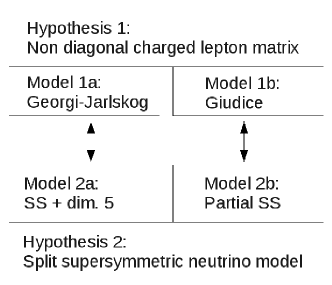
Figure 1: Conceptual flow chart of how the basic ideas of a non-diagonal charge lepton Yukawa matrix and split-supersymmetric neutrino models are combined and studied.

A priory there is no restriction when combining models for charged leptons with models for neutrinos. We decided to study two specific examples as shown in figure 1.

II NEUTRAL AND CHARGED FERMIONS IN BRPV

In the supersymmetric models we are studying here, tree-level contributions to neutrino masses and mixings arise from the neutrino-neutralino mixing due to bilinear R-parity violation. In general, when writing down the gauge invariant terms that violate R-parity one can consider Lagrange terms that contain three fields (trilinear) and terms that contain two fields (bilinear). In the context of SS all the trilinear terms are irrelevant since they contain heavy scalars that are integrated out of the effective theory.

In BRpV models neutralinos mix with neutrinos such that a $7\times 7$ mass matrix is generated. In the base $\psi_{0}^{T}=(-i\widetilde{B},i\widetilde{W}^{0},\widetilde{H}_{d}^{0},\widetilde{H}_{u}^{0},\nu_{e},\nu_{\mu},\nu_{\tau})$ the corresponding terms in the lagrangian are grouped as,

$${\cal L}_{N}=-\frac{1}{2}(\psi^{0})^{T}{\cal M}_{N}\psi^{0}$$ (1)

with the mass matrix introduced in blocks hep-ph/0302021 ,

$${\cal M}_{N}=\left(\begin{array}[]{cc}{\mathrm{M}}_{\chi^{0}}&m^{T}\\ m&0\end{array}\right),$$ (2)

This neutralino/neutrino mass matrix is diagonalized with the rotation matrix,

$${\cal N}=\left(\begin{matrix}N&0\cr 0&U_{\nu}^{T}\end{matrix}\right)\left(\begin{matrix}1-\frac{1}{2}\xi^{T}\xi&\xi^{T}\cr-\xi&1-\frac{1}{2}\xi\xi^{T}\end{matrix}\right)\equiv\left(\begin{matrix}N&0\cr 0&U_{\nu}^{T}\end{matrix}\right){\cal N}_{\xi}$$ (3)

with $\xi=m{\mathrm{M}}_{\chi^{0}}^{-1}$ at first order in perturbation theory. The matrix ${\cal N}_{\xi}$ allows a block diagonalization such that,

$${\cal N}_{\xi}{\cal M}_{N}{\cal N}_{\xi}^{T}=\left(\begin{matrix}{\mathrm{M}}_{\chi^{0}}&0\cr 0&{\mathrm{M}}_{\nu}^{eff}\end{matrix}\right)$$ (4)

with ${\mathrm{M}}_{\nu}^{eff}=-m{\mathrm{M}}_{\chi^{0}}^{-1}m^{T}$. Matrices $N$ and $U_{\nu}$ further diagonalize the neutralino mass matrix ${\mathrm{M}}_{\chi^{0}}$ and the effective neutrino mass matrix ${\mathrm{M}}_{\nu}^{eff}$ respectively:

$$\left(\begin{array}[]{cc}N&0\\ 0&U^{T}_{\nu}\end{array}\right)\left(\begin{array}[]{cc}{\mathcal{M}}_{\bar{\chi}^{0}}&0\\ 0&{\mathcal{M}}_{\nu}^{eff}\end{array}\right)\left(\begin{array}[]{cc}N^{T}&0\\ 0&U_{\nu}\end{array}\right)=\left(\begin{array}[]{cc}{\mathcal{M}}_{\bar{\chi}^{0}}^{diag}&0\\ 0&{\mathcal{M}}_{\nu}^{diag}\end{array}\right)$$ (5)

We call these eigenstates $F^{0}_{i}$ with $i=1,...7$.

As we will see, in order to correctly define the neutrino mixing angles we need to study the charged lepton sector as well. In BRpV charginos mix with charged leptons forming the following mass terms,

$${\cal L}_{C}=-\frac{1}{2}\left(\psi^{+T},\psi^{-T}\right)\left(\begin{matrix}0&{\cal M}_{C}^{T}\cr{\cal M}_{C}&0\end{matrix}\right)\left(\begin{matrix}\psi^{+}\cr\psi^{-}\end{matrix}\right)$$ (6)

where the basis is $\psi^{-T}=(-i\widetilde{W}^{-},\widetilde{H}_{d}^{-},e_{L}^{-},\mu_{L}^{-},\tau_{L}^{-})$ and $\psi^{-T}=(-i\widetilde{W}^{+},\widetilde{H}_{u}^{+},e_{R}^{+},\mu_{R}^{+},\tau_{R}^{+})$. We divide the $5\times 5$ mass matrix into blocks hep-ph/0302021 ,

$${\cal M}_{C}=\left(\begin{matrix}M_{\chi^{+}}&Y\cr m_{c}&M_{\ell}\end{matrix}\right)$$ (7)

This chargino/charged lepton mass matrix is not symmetric thus it is diagonalized by two matrices

$${\cal U}{\cal M}_{C}{\cal V}^{T}={\cal M}_{C}^{diag}$$ (8)

where we first look for a block diagonalization, as in the neutral case, performed by matrices ${\cal U}_{\xi}$ and ${\cal V}_{\xi}$. Neglecting $Y$ (small Yukawa couplings and sneutrino vevs) we find,

$${\cal U}_{\xi}=\left(\begin{matrix}1-\frac{1}{2}\xi_{L}^{T}\xi_{L}&\xi_{L}^{T}\cr-\xi_{L}&1-\frac{1}{2}\xi_{L}\xi_{L}^{T}\end{matrix}\right)\,,\qquad{\cal V}_{\xi}=\left(\begin{matrix}1-\frac{1}{2}\xi_{R}^{T}\xi_{R}&\xi_{R}^{T}\cr-\xi_{R}&1-\frac{1}{2}\xi_{R}\xi_{R}^{T}\end{matrix}\right)$$ (9)

with $\xi_{L}=m_{c}M_{\chi^{+}}^{-1}$ and $\xi_{R}=M_{\ell}m_{c}M_{\chi^{+}}^{-1}(M_{\chi^{+}}^{-1})^{T}$. In the small lepton masses and small BRpV parameters approximation, $\xi_{R}$ can be neglected. This implies that to first order on BRpV parameters the chargino and the charged lepton mass matrices are unchanged by the block diagonalization,

$$M_{\chi^{+}}^{eff}=M_{\chi^{+}}\,,\qquad M_{\ell}^{eff}=M_{\ell}$$ (10)

The full diagonalization is accomplished with,

$${\cal U}=\left(\begin{matrix}U&0\cr 0&V_{L}\end{matrix}\right){\cal U}_{\xi}\,,\qquad{\cal V}=\left(\begin{matrix}V&0\cr 0&V_{R}\end{matrix}\right){\cal V}_{\xi}$$ (11)

where

$$UM_{\chi^{+}}V^{T}=M_{\chi^{+}}^{diag}\,,\qquad V_{L}M_{\ell}V_{R}^{T}=M_{\ell}^{diag}$$ (12)

The matrices $M_{\chi^{+}}^{diag}$ and $M_{\ell}^{diag}$ contain the final chargino and charged lepton masses. We call these eigenstates $F^{\pm}_{i}$ with $i=1,...5$.

III GUT motivated Ansatz for Charged Leptons Mass Matrix

Grand Unified Theories provide a well motivated framework to study non-diagonal charged lepton mass matrices. The most studied Grand Unification gauge groups are $SU(5)$ and $SO(10)$, which break down to the SM gauge group $SU(3)\times SU(2)\times U(1)$. In addition, the GUT can be embedded into supersymmetry. In this context, different proposals for a charged lepton mass matrix are postulated at the GUT scale. In the following subsections we will study two GUT examples based on the two groups mentined above.

III.1 Georgi-Jarlskog Ansatz

We consider first the Georgi-Jarlskog ansatz Georgi:1979df for the charged lepton mass matrix, introduced in the context of an $SU(5)$ GUT theory, and re-analyzed in Dimopoulos:1991za for a supersymmetric $SO(10)$ GUT group. Written in the notation of the later article, the charged lepton mass matrix depends on three parameters $D$, $E$, and $F$, which we assume real. We have,

$$M_{\ell}=\frac{v}{\sqrt{2}}\left(\begin{matrix}0&F&0\cr F&-3E&0\cr 0&0&D\end{matrix}\right)$$ (13)

which essentially does not change after RGE running effects. The matrix is proportional to $v$ when the low energy theory contains only one Higgs doublet (for example Split Supersymmetry). In the case it contains two Higgs doublets (for example Partial Split Supersymmetry) the replacement $v\rightarrow v_{d}$ must be made.

If we assume $E$ is positive, the eigenvalues are,

$$m_{\ell_{1}} = \frac{v}{2\sqrt{2}}\left(-3E+\sqrt{9E^{2}+4F^{2}}\right)$$

$$m_{\ell_{2}} = \frac{v}{2\sqrt{2}}\left(-3E-\sqrt{9E^{2}+4F^{2}}\right)$$ (14)

$$m_{\ell_{3}} = \frac{v}{\sqrt{2}}D$$

These eigenvalues, up to a possible sign, are equal to $m_{e}=0.511$ MeV, $m_{\mu}=105.7$ MeV, and $m_{\tau}=1777$ MeV respectively Nakamura:2010zzi , fixing the parameters in the charged lepton Yukawa matrix to $F=4.22\times 10^{-5}$, $E=2.01\times 10^{-4}$, and $D=1.02\times 10^{-2}$.

It is clear that only one angle is enough to parametrize $M_{\ell}^{diag}=V_{L}M_{\ell}V_{R}^{T}$. Since $M_{\ell}$ is symmetric, the diagonalization matrix has the following form,

$$V_{L}=V_{R}=\left(\begin{matrix}\cos\alpha&\sin\alpha&0\cr-\sin\alpha&\cos\alpha&0\cr 0&0&1\end{matrix}\right)\,,\qquad\tan 2\alpha=\frac{2F}{3E}$$ (15)

This angle is such that $\sin\alpha\approx 0.0695$.

III.2 Giudice Ansatz

The second ansatz we consider was introduced by G. Giudice Giudice:1992an in the context of supersymmetric Grand Unified Theories (GUT). The charged lepton mass matrix is,

$$M^{\prime}_{\ell}=\frac{v_{d}}{\sqrt{2}}\left(\begin{matrix}0&F&0\cr F&-3E&2E\cr 0&2E&D\end{matrix}\right)$$ (16)

whose Yukawa couplings do not change after running. The implications of this type of ansatz in terms of neutrino textures have been investigated in hep-ph/9409369 ; hep-ph/9509351 ; hep-ph/0012046 . We will associate this ansatz with Partial Split Supersymmetry, hence the mass matrix is proportional to $v_{d}$. The hierarchical nature of the charged lepton and quarks necessitates $F\ll E\ll D$. In this approximation we find the following eigenvalues,

$$m_{\ell_{1}} \approx \frac{v_{d}}{\sqrt{2}}\,\frac{F^{2}}{3E}$$

$$m_{\ell_{2}} \approx \frac{v_{d}}{\sqrt{2}}\left(-3E-4\frac{E^{2}}{D}\right)$$ (17)

$$m_{\ell_{3}} \approx \frac{v_{d}}{\sqrt{2}}\left(D+4\frac{E^{2}}{D}\right)$$

Imposing the experimental values of the charged leptons into these results we find $Fc_{\beta}=4.17\times 10^{-5}$, $Ec_{\beta}=1.97\times 10^{-4}$, and $Dc_{\beta}=1.02\times 10^{-2}$. Note that these Yukawa parameters grow with $\tan\beta$. Notice also that the numerical value of the parameters $F$, $E$, and $C$ differ only slightly with respect to the ones obtained for the previous ansatz (for $v=v_{d}\Leftrightarrow\cos\beta=1$). This is related to the fact that the charged lepton masses are hierarchical.

The mass matrix $M^{\prime}_{\ell}$ in eq. (16) is diagonalized by the following matrix,

$$V^{\prime}_{L}=V^{\prime}_{R}\approx\left(\begin{matrix}1&-\frac{F}{3E}&0\cr\frac{F}{3E}&1&\frac{2E}{D}\cr 0&-\frac{2E}{D}&1\end{matrix}\right)$$ (18)

where we have neglected smaller terms. We parametrize this rotation matrix with two angles,

$$V_{L}^{\prime}=\left(\begin{matrix}\cos\alpha^{\prime}&\sin\alpha^{\prime}&0\cr-\sin\alpha^{\prime}&\cos\alpha^{\prime}&0\cr 0&0&1\end{matrix}\right)\left(\begin{matrix}1&0&0\cr 0&\cos\theta^{\prime}&\sin\theta^{\prime}\cr 0&-\sin\theta^{\prime}&\cos\theta^{\prime}\end{matrix}\right)\,,\quad\tan 2\alpha^{\prime}\approx\frac{2F}{3E}\,,\quad\tan 2\theta^{\prime}\approx-\frac{4E}{D}$$ (19)

These angles are such that $\sin\alpha^{\prime}\approx 0.070$ and $\sin\theta^{\prime}\approx 0.036$. Notice that $V_{L}^{\prime}(\theta^{\prime}=0,\alpha^{\prime}=\alpha)=V_{L}(\alpha)$.

IV ${\bf U_{PMNS}}$ and ${\bf W}$ Boson Coupling to Fermions

Charged and neutral fermion couplings to the $W$ boson are essential for the $U_{PMNS}$ matrix of neutrino mixing angles because they define the base where charged leptons are diagonal. In BRpV models the situation is complicated by the fact that charginos mix with charged leptons, as we saw in the previous chapter. The relevant coupling is,

$=\,i\,\gamma^{\mu}\,\Big{[}O^{cnw}_{Lij}\frac{(1-\gamma_{5})}{2}+O^{cnw}_{Rij}\frac{(1+\gamma_{5})}{2}\Big{]}$

with

$$O_{Lij}^{cnw} = -g\bigg{[}{\cal N}_{j2}\,{\cal U}_{i1}+\frac{1}{\sqrt{2}}\Big{(}{\cal N}_{j3}\,{\cal U}_{i2}+\sum_{k=1}^{3}{\cal N}_{j,4+k}\,{\cal U}_{i,2+k}\Big{)}\bigg{]}$$

$$O_{Rij}^{cnw} = -g\bigg{[}{\cal N}_{j2}\,{\cal V}_{i1}+\frac{1}{\sqrt{2}}\,{\cal N}_{j4}\,{\cal V}_{i2}\bigg{]}$$ (20)

In first approximation in $\epsilon/M_{\chi}$ we use,

$${\cal N}=\left(\begin{matrix}N&N\xi^{T}\cr-U_{\nu}^{T}\xi&U_{\nu}^{T}\end{matrix}\right)\,,\qquad{\cal U}=\left(\begin{matrix}U&U\xi_{L}^{T}\cr-V_{L}\xi_{L}&V_{L}\end{matrix}\right)\,,\qquad{\cal V}=\left(\begin{matrix}V&0\cr 0&V_{R}\end{matrix}\right)$$ (21)

and find for the charged lepton and neutrino coupling to $W$ Bosons the following,

$=\,-i\,\frac{g}{\sqrt{2}}\,\left(V_{L}U_{\nu}\right)_{ij}\,\gamma^{\mu}\,\frac{(1-\gamma_{5})}{2}$

Therefore, the neutrino mixing angles are defined by,

$$U_{PMNS}=V_{L}U_{\nu}$$ (22)

Notice that the $U_{PMNS}$ matrix coincides with the matrix that diagonalizes the neutrino mass matrix, $U_{\nu}$, only when the charged leptons are diagonal in the original basis. Otherwise, there is an extra contribution from the left matrix $V_{L}$ that diagonalizes the charged lepton mass matrix.

Using the following convention for the neutrino angles,

$$U_{PMNS}=\left(\begin{matrix}1&0&0\cr 0&c_{23}&s_{23}\cr 0&-s_{23}&c_{23}\end{matrix}\right)\left(\begin{matrix}c_{13}&0&s_{13}e^{i\delta}\cr 0&1&0\cr-s_{13}e^{-i\delta}&0&c_{13}\end{matrix}\right)\left(\begin{matrix}c_{12}&s_{12}&0\cr-s_{12}&c_{12}&0\cr 0&0&1\end{matrix}\right)$$ (23)

and assuming this matrix is real ($\delta=0$), the general structure for the mixing angles considering the Giudice ansatz for the charged leptons (19) is given by,

$$\sin\theta_{13}^{(V^{\prime}_{L}\neq 1)} = \sin\theta_{13}^{(V^{\prime}_{L}=1)}+s^{\prime}_{\alpha}s_{23}c_{13}$$

$$\tan\theta_{23}^{(V^{\prime}_{L}\neq 1)} = \tan\theta_{23}^{(V^{\prime}_{L}=1)}\left\{1+s^{\prime}_{\theta}\left(t_{23}+\frac{1}{t_{23}}\right)-s^{\prime}_{\alpha}\frac{t_{13}}{s_{23}}\right\}$$

$$\tan\theta_{12}^{(V^{\prime}_{L}\neq 1)} = \tan\theta_{12}^{(V^{\prime}_{L}=1)}\left\{1+s^{\prime}_{\alpha}\frac{c_{23}}{c_{13}}\left(t_{12}+\frac{1}{t_{12}}\right)\right\}$$ (24)

where we have used the fact that the angles $\alpha^{\prime}$ and $\theta^{\prime}$ are small. Analogous expressions for the Georgi-Jarlskog ansatz are obtained by the substitution $V^{\prime}_{L}\rightarrow V_{L}$, $\theta^{\prime}=0$, and $\alpha^{\prime}\rightarrow\alpha$.

V Split Supersymmetry with Flavor Blind Dimension Five

In Split Supersymmetry ArkaniHamed:2004fb all scalars are very heavy, for simplicity degenerated at a mass $\tilde{m}$, except for one Higgs doublet. Integrating out the heavy scalars the SS Lagrangian includes,

$${\mathcal{L}}_{SS} \owns-\Big{[}m^{2}H^{{\dagger}}H+\frac{\lambda}{2}(H^{{\dagger}}H)^{2}\Big{]}-Y_{u}\overline{Q}_{L}u_{R}i\sigma_{2}H^{*}-Y_{d}\overline{Q}_{L}d_{R}H-Y_{e}\overline{L}_{L}e_{R}H$$

$$-\frac{M_{3}}{2}\tilde{G}\tilde{G}-\frac{M_{2}}{2}\tilde{W}\tilde{W}-\frac{M_{1}}{2}\widetilde{B}\widetilde{B}-\mu\widetilde{H}^{T}_{u}i\sigma_{2}\widetilde{H}_{d}-\frac{1}{\sqrt{2}}H^{{\dagger}}(\widetilde{g}_{u}\sigma\widetilde{W}+\tilde{g}^{\prime}_{u}\widetilde{B})\widetilde{H}_{u}$$

$$-\frac{1}{\sqrt{2}}H^{T}i\sigma_{2}(-\widetilde{g}_{d}\sigma\widetilde{W}+\widetilde{g}^{\prime}_{d}\widetilde{B})\widetilde{H}_{d}+\mathrm{h.c},$$ (25)

The last two terms are the Higgs-gaugino-higgsino interactions, with couplings $\tilde{g}$ induced by integrating out the heavy scalars.

Split Supersymmetry with violation of R-Parity Diaz:2006ee includes the extra terms

$${\cal L}_{SS}^{RpV}\owns\epsilon_{i}\widetilde{H}^{T}_{u}i\sigma_{2}L_{i}-\frac{1}{\sqrt{2}}a_{i}H^{T}i\sigma_{2}(-\tilde{g}_{d}\sigma\widetilde{W}+\tilde{g}^{\prime}_{d}\widetilde{B})L_{i}\ +\ \mathrm{h.c.}.$$ (26)

The first term corresponds to the usual bilinear violation of R-Parity, which mixes higgsinos with leptons through the mass parameters $\epsilon_{i}$. The terms proportional to the $a_{i}$ parameters are generated as effective terms in the SS lagrangian after integrating out the sfermions.

V.1 Neutrinos and Neutralinos in SS

Now we specify the neutrino-neutralino mixing described in section II for the Split Supersymmetric case. The upper left block in eq. (4) corresponds to the neutralino sector,

$${\bf M}_{\chi^{0}}^{SS}=\left(\begin{array}[]{cccc}M_{1}&0&-\frac{1}{2}\tilde{g}^{\prime}_{d}v&\frac{1}{2}\tilde{g}^{\prime}_{u}v\\ 0&M_{2}&\frac{1}{2}\tilde{g}_{d}v&-\frac{1}{2}\tilde{g}_{u}v\\ -\frac{1}{2}\tilde{g}^{\prime}_{d}v&\frac{1}{2}\tilde{g}_{d}v&0&-\mu\\ \frac{1}{2}\tilde{g}^{\prime}_{u}v&-\frac{1}{2}\tilde{g}_{u}v&-\mu&0\end{array}\right)$$ (27)

where $M_{1},M_{2}$ are the gaugino masses, $\mu$ is the higgsino mass, and $v=246$ GeV is the Higgs vacuum expectation value. The neutralino/neutrino mixing is equal to,

$$m^{SS}=\left(\begin{array}[]{cccc}-\frac{1}{2}\tilde{g}^{\prime}_{d}a_{1}v&\frac{1}{2}\tilde{g}_{d}a_{1}v&0&\epsilon_{1}\cr-\frac{1}{2}\tilde{g}^{\prime}_{d}a_{2}v&\frac{1}{2}\tilde{g}_{d}a_{2}v&0&\epsilon_{2}\cr-\frac{1}{2}\tilde{g}^{\prime}_{d}a_{3}v&\frac{1}{2}\tilde{g}_{d}a_{3}v&0&\epsilon_{3}\end{array}\right).$$ (28)

with $\epsilon_{i}$ and $a_{i}$ the BRpV parameters described in eq. (26). Therefore, in Split Supersymmetry the effective neutrino mass matrix is given by,

$${\bf M}_{\nu}^{eff}=-m^{SS}\,({\mathrm{M}}_{\chi^{0}}^{SS})^{-1}\,(m^{SS})^{T}=\frac{v^{2}}{4\det{M_{\chi^{0}}^{SS}}}\left(M_{1}\tilde{g}^{2}_{d}+M_{2}\tilde{g}^{\prime 2}_{d}\right)\left(\begin{array}[]{cccc}\lambda_{1}^{2}&\lambda_{1}\lambda_{2}&\lambda_{1}\lambda_{3}\cr\lambda_{2}\lambda_{1}&\lambda_{2}^{2}&\lambda_{2}\lambda_{3}\cr\lambda_{3}\lambda_{1}&\lambda_{3}\lambda_{2}&\lambda_{3}^{2}\end{array}\right),$$ (29)

with $\lambda_{i}=a_{i}\mu+\epsilon_{i}$. The determinant of the neutralino mass matrix is found to be,

$$\det{M_{\chi^{0}}^{SS}}=-\mu^{2}M_{1}M_{2}+\frac{1}{2}v^{2}\mu\left(M_{1}\tilde{g}_{u}\tilde{g}_{d}+M_{2}\tilde{g}^{\prime}_{u}\tilde{g}^{\prime}_{d}\right)+\textstyle{\frac{1}{16}}v^{4}\left(\tilde{g}^{\prime}_{u}\tilde{g}_{d}-\tilde{g}_{u}\tilde{g}^{\prime}_{d}\right)^{2}.$$ (30)

For our numerical calculations we neglect the running of the $\tilde{g}$ couplings.

Since the effective neutrino mass matrix has only one non-zero eigenvalue, at tree level only the atmospheric mass squared is generated, and the solar mass squared difference remains null. In Split Supersymmetry this does not change when we add quatum corrections to the neutrino mass matrix. This is a well known fact in BRpV Split Supersymmetry Davidson:2000ne . Nevertheless, it has been noticed that gravity contributions via dimension 5 operators, can generate a solar mass when the operator is suppressed by a reduced Planck mass, as in models with extra dimensions Berezinsky:2004zb . Following ref. Diaz:2009yz , we include a contribution to the neutrino mass matrix induced by gravity,

$$M_{\nu}^{G}=\mu_{g}\left(\begin{matrix}1&1&1\cr 1&1&1\cr 1&1&1\end{matrix}\right)$$ (31)

where $\mu_{g}\sim v^{2}/M_{X}$ parametrizes the size of the contribution. This parameter has units of mass, is proportional to the Higgs vacuum expectation value squared $v^{2}$, and inversely proportional to the reduced Planck mass $M_{X}$. The equality of all entries in the matrix symbolizes the expected flavor blindness of the gravitational interactions.

Assuming that the charged lepton mass matrix is already diagonal, it was shown in ref. Diaz:2009yz that neutrino mass squared differences predict values $\mu_{g}\sim 3\times 10^{-3}$ eV. This corresponds to a reduced Planck mass $M_{X}\sim 2\times 10^{16}$ GeV, remarkably close to the GUT mass scale. In addition, maximal atmospheric mixing predicts $\sin^{2}\theta_{sol}=1/3$, well within the $3\sigma$ experimental result $\sin^{2}\theta_{sol}=0.305\pm 0.075$. In the following we will explore the effects of a non-diagonal charged lepton mass matrix.

V.2 Charged Leptons and Charginos in SS

In SS the chargino block in equation (7) has the following structure,

$$M_{\chi^{+}}=\left(\begin{matrix}M_{2}&\frac{1}{\sqrt{2}}\tilde{g}_{u}v\cr\frac{1}{\sqrt{2}}\tilde{g}_{d}v&\mu\end{matrix}\right)$$ (32)

with all the parameters already defined in the previous sections. The charged lepton mass matrix has the usual form $M_{\ell}^{ij}=Y_{\ell}^{ij}v/\sqrt{2}$, with $Y_{\ell}$ the lepton Yukawa couplings.

The mixing between charginos and charged leptons is given by the matrices

$$m_{c}=\left(\begin{matrix}\frac{1}{\sqrt{2}}\tilde{g}_{d}a_{1}v&-\epsilon_{1}\cr\frac{1}{\sqrt{2}}\tilde{g}_{d}a_{2}v&-\epsilon_{2}\cr\frac{1}{\sqrt{2}}\tilde{g}_{d}a_{3}v&-\epsilon_{3}\cr\end{matrix}\right)$$ (33)

and

$$Y=\left(\begin{matrix}0&0&0\cr-\frac{1}{\sqrt{2}}Y_{\ell}^{1i}a_{i}v&-\frac{1}{\sqrt{2}}Y_{\ell}^{2i}a_{i}v&-\frac{1}{\sqrt{2}}Y_{\ell}^{3i}a_{i}v\cr\end{matrix}\right)$$ (34)

Since lepton masses are so much smaller than chargino masses and R-Parity violating terms $a_{i}$ are also small, it is usually a good approximation to neglect the effect of the matrix $Y$, as we did in the diagonalization process in section II.

Notice that the charged lepton Yukawa matrix does not need to be diagonal. This point is not trivial, and has consequences on the neutrino mixing angles as we will see in the next chapters.

V.3 Effects on Neutrino Parameters in SS

The effective neutrino mass matrix, including BRpV terms and a gravity induced contribution from a flavor blind dimension 5 operator in models with extra dimensions, is

$$M_{\nu}^{ij}=A_{\lambda}\lambda^{i}\lambda^{j}+\mu_{g}\,.$$ (35)

It is obtained by summing eqs. (29) and (31), with the coefficient $A_{\lambda}$ being read from eq. (29). The neutrino mass parameters are not changed by the charged lepton contributions Diaz:2009yz ,

$$\Delta m^{2}_{sol} = \mu_{g}^{2}\frac{|\vec{v}\times\vec{\lambda}|^{4}}{|\vec{\lambda}|^{4}}+{\mathcal{O}}(\mu_{g}^{3})$$

$$\Delta m^{2}_{atm} = A_{\lambda}^{2}|\vec{\lambda}|^{4}+2A_{\lambda}\mu_{g}(\vec{v}\cdot\vec{\lambda})^{2}+{\mathcal{O}}(\mu_{g}^{2})$$ (36)

but the mixing angles are corrected. Considering the diagonalization matrix from Georgi-Jarlskog ansatz in eq. (15), and using the convention in eq. (23) for neutrino angles, we find

$$\sin\theta_{13} = \frac{c\lambda_{1}+s\lambda_{2}}{|\vec{\lambda}|}$$ (37)

$$\tan\theta_{23} = \frac{c\lambda_{2}-s\lambda_{1}}{\lambda_{3}}$$

$$\tan\theta_{12} = \frac{1}{|\vec{\lambda}|}\left[\frac{c(\lambda_{2}^{2}+\lambda_{3}^{2}-\lambda_{1}\lambda_{2}-\lambda_{1}\lambda_{3})+s(\lambda_{1}^{2}+\lambda_{3}^{2}-\lambda_{1}\lambda_{2}-\lambda_{2}\lambda_{3})}{c(\lambda_{3}-\lambda_{2})+s(\lambda_{1}-\lambda_{2})}\right]$$

where $c=\cos\alpha$ and $s=\sin\alpha$. These relations are a special case of the general formulae in eq. (24).

From this we can learn the following. First, the $3\sigma$ upper bound $\sin^{2}\theta_{13}<0.035$ Schwetz:2011zk implies that a good approximation, as in Diaz:2009yz , is $\lambda_{1}^{2}\ll\lambda_{2}^{2}+\lambda_{3}^{2}$. Therefore, the correction on $\sin^{2}\theta_{13}$ may be very significant since both terms in $c\lambda_{1}+s\lambda_{2}$ are comparable. Second, the correction on the atmospheric angle is of a second order, since $s$ and $\lambda_{1}/|\vec{\lambda}|$ are small. Third, the correction on the solar angle is typically of the order of $s$ ($\sim 7\%$), which is not negligible. In section VII these effects are studied numerically.

VI Partial Split Supersymmetry

In Partial Split Supersymmetry all sfermions are heavy, for simplicity degenerate with a mass $\widetilde{m}$, while the two Higgs doublets remain at the weak scale Diaz:2006ee ; Diaz:2009gf ; Sundrum:2009gv . The lagrangian includes,

$${\cal L}_{PSS} \owns -\Big{[}m_{1}^{2}H_{d}^{\dagger}H_{d}+m_{2}^{2}H_{u}^{\dagger}H_{u}-m_{12}^{2}(H_{d}^{T}\epsilon H_{u}+h.c.)$$

$$+\textstyle{\frac{1}{2}}\lambda_{1}(H_{d}^{\dagger}H_{d})^{2}+\textstyle{\frac{1}{2}}\lambda_{2}(H_{u}^{\dagger}H_{u})^{2}+\lambda_{3}(H_{d}^{\dagger}H_{d})(H_{u}^{\dagger}H_{u})+\lambda_{4}|H_{d}^{T}\epsilon H_{u}|^{2}\Big{]}$$

$$+Y_{u}\overline{u}_{R}H_{u}^{T}\epsilon q_{L}-Y_{d}\overline{d}_{R}H_{d}^{T}\epsilon q_{L}-Y_{e}\overline{e}_{R}H_{d}^{T}\epsilon l_{L}$$

$$-\textstyle{\frac{1}{\sqrt{2}}}H_{u}^{\dagger}(\tilde{g}_{u}\sigma\widetilde{W}+\tilde{g}^{\prime}_{u}\widetilde{B})\widetilde{H}_{u}-\textstyle{\frac{1}{\sqrt{2}}}H_{d}^{\dagger}(\tilde{g}_{d}\sigma\widetilde{W}-\tilde{g}^{\prime}_{d}\widetilde{B})\widetilde{H}_{d}+\mathrm{h.c.}$$

The first two lines correspond to the Higgs potential of a two Higgs doublet model, where the quartic couplings have boundary conditions at $\widetilde{m}$ that connect to the supersymmetric models above $\widetilde{m}$. In the third line we include the Yukawa couplings, while in the forth one we have the Higgs-higgsino-gaugino couplings. These $Y$ and $\tilde{g}$ couplings in PSS differ from the corresponding ones in SS in their RGE and their boundary conditions at $\widetilde{m}$.

BRpV is introduced in PSS with the terms,

$${\cal L}_{PSS}^{RpV}=\epsilon_{i}\widetilde{H}_{u}^{T}\epsilon L_{i}\ -\ {\frac{1}{\sqrt{2}}}b_{i}H_{u}^{T}\epsilon(\tilde{g}_{d}\sigma\widetilde{W}-\tilde{g}^{\prime}_{d}\widetilde{B})L_{i}\ +\ h.c.,$$ (39)

where the origin of the second term is analogous as in SS: they are generated as effective terms after integrating out the heavy sfermions.

VI.1 Neutrinos and Neutralinos in PSS

The neutralino sector of the neutrino/neutralino mass matrix in PSS has the following form,

$${\bf M}_{\chi^{0}}^{PSS}=\left(\begin{array}[]{cccc}M_{1}&0&-\frac{1}{2}\tilde{g}^{\prime}_{d}v_{d}&\frac{1}{2}\tilde{g}^{\prime}_{u}v_{u}\\ 0&M_{2}&\frac{1}{2}\tilde{g}_{d}v_{d}&-\frac{1}{2}\tilde{g}_{u}v_{u}\\ -\frac{1}{2}\tilde{g}^{\prime}_{d}v_{d}&\frac{1}{2}\tilde{g}_{d}v_{d}&0&-\mu\\ \frac{1}{2}\tilde{g}^{\prime}_{u}v_{u}&-\frac{1}{2}\tilde{g}_{u}v_{u}&-\mu&0\end{array}\right).$$ (40)

It differs only slightly from SS in eq. (27): it is apparent in eq. (40) that there are two different vacuum expectation values, as in the MSSM, and as it was mentioned before the $\tilde{g}$ couplings have different RGE and boundary conditions. The mixing sub-matrix has also only minor differences,

$$m^{PSS}=\left(\begin{array}[]{cccc}-\frac{1}{2}\tilde{g}^{\prime}_{d}b_{1}v_{u}&\frac{1}{2}\tilde{g}_{d}b_{1}v_{u}&0&\epsilon_{1}\cr-\frac{1}{2}\tilde{g}^{\prime}_{d}b_{2}v_{u}&\frac{1}{2}\tilde{g}_{d}b_{2}v_{u}&0&\epsilon_{2}\cr-\frac{1}{2}\tilde{g}^{\prime}_{d}b_{3}v_{u}&\frac{1}{2}\tilde{g}_{d}b_{3}v_{u}&0&\epsilon_{3}\end{array}\right),$$ (41)

The neutrino effective mass matrix in PSS takes the form,

$${\bf M}_{\nu}^{eff}=\frac{M_{1}\tilde{g}^{2}_{d}+M_{2}\tilde{g}^{\prime 2}_{d}}{4\det{M_{\chi^{0}}^{PSS}}}\left(\begin{array}[]{cccc}\Lambda_{1}^{2}&\Lambda_{1}\Lambda_{2}&\Lambda_{1}\Lambda_{3}\cr\Lambda_{2}\Lambda_{1}&\Lambda_{2}^{2}&\Lambda_{2}\Lambda_{3}\cr\Lambda_{3}\Lambda_{1}&\Lambda_{3}\Lambda_{2}&\Lambda_{3}^{2}\end{array}\right),$$ (42)

with $\Lambda_{i}=\mu b_{i}v_{u}+\epsilon_{i}v_{d}$, and with the determinant of the neutralino submatrix equal to,

$$\det{M_{\chi^{0}}^{PSS}}=-\mu^{2}M_{1}M_{2}+\frac{1}{2}v_{u}v_{d}\mu\left(M_{1}\tilde{g}_{u}\tilde{g}_{d}+M_{2}\tilde{g}^{\prime}_{u}\tilde{g}^{\prime}_{d}\right)+\textstyle{\frac{1}{16}}v_{u}^{2}v_{d}^{2}\left(\tilde{g}^{\prime}_{u}\tilde{g}_{d}-\tilde{g}_{u}\tilde{g}^{\prime}_{d}\right)^{2}.$$ (43)

Despite these differences, the tree-level neutrino mass matrix in eq. (42) also has only one non-zero eigenvalue, generating an atmospheric mass difference but not a solar mass difference. Nevertheless, as oppose to the SS case, in PSS quantum corrections do lift the symmetry of the tree-level matrix, generating a corrected neutrino mass matrix that looks like,

$$M_{\nu}^{ij}=A\Lambda_{i}\Lambda_{j}+C\epsilon_{i}\epsilon_{j},$$ (44)

where the tree-level value $A^{(0)}$ can be read from eq. (42). One-loop diagrams corrects it into the value $A$, and generate the constant $C$. The matrix in eq. (44) has only one null eigenvalue, thus a non-zero atmospheric and solar mass difference. A quadratic constant $B$ that mixes $\Lambda_{i}$ and $\epsilon_{j}$ is also generated in general, but can be adjusted to zero by choosing an appropriate value for the arbitrary renormalization scale of dimensional regularization.

This mechanism depends strongly on the $b_{i}$ terms in the definition of $\Lambda_{i}$. The origin of those terms is that above the splitting scale $\tilde{m}$ the Higgs scalars gauge eigenstates mix with sneutrinos gauge eigenstates. This happens for the CP-even real parts and the CP-odd imaginary parts. Due to this mixing one might define the real part of sneutrinos ($s^{i}_{s},\,t^{i}_{s}$) in the CP-even Higgs mass eigenstates ($h,\,H$). It has been shown that for the real part $s^{i}_{s}\sim-b_{i}c_{\alpha}\sim-c_{\alpha}v_{i}/v_{u}$ and that $t^{i}_{s}\sim-b_{i}s_{\alpha}\sim-s_{\alpha}v_{i}/v_{u}$. The relations for the imaginary parts are analogous Diaz:2006ee . Thus, the existence of a non-zero $b_{i}$ term in indicates that actually Higgs Bosons, at any energy scale below $\tilde{m}$ will have a small sneutrino component. This means that the sneutrinos are not completely decoupled at those scales. It is further instructive to notice that the $b_{i}$ are proportional to the sneutrino vacuum expectation value, which implies that it disappears for a restored $SU(2)$ symmetry. This fact is important in order to understand this model in context of some general theorems on neutrino masses Weinberg:1979sa ; hep-ph/9701253 .

VI.2 Charged Leptons and Charginos in PSS

The chargino block in PSS has the following structure,

$$M_{\chi^{+}}=\left(\begin{matrix}M_{2}&\frac{1}{\sqrt{2}}\tilde{g}_{u}v_{u}\cr\frac{1}{\sqrt{2}}\tilde{g}_{d}v_{d}&\mu\end{matrix}\right)$$ (45)

The difference with the SS case in eq. (32) lies in the fact that now we have two vacuum expectation values $v_{u}$ and $v_{d}$ (as in the MSSM), and that the $\tilde{g}$ couplings, defined in eq. (VI), are numerically different.

The mixing between charginos and charged leptons is given by the matrices

$$m_{c}=\left(\begin{matrix}\frac{1}{\sqrt{2}}\tilde{g}_{d}b_{1}v_{d}&-\epsilon_{1}\cr\frac{1}{\sqrt{2}}\tilde{g}_{d}b_{2}v_{d}&-\epsilon_{2}\cr\frac{1}{\sqrt{2}}\tilde{g}_{d}b_{3}v_{d}&-\epsilon_{3}\cr\end{matrix}\right)$$ (46)

and

$$Y=\left(\begin{matrix}0&0&0\cr-\frac{1}{\sqrt{2}}Y^{\prime 1i}_{\ell}b_{i}v_{d}&-\frac{1}{\sqrt{2}}Y^{\prime 2i}_{\ell}b_{i}v_{d}&-\frac{1}{\sqrt{2}}Y^{\prime 3i}_{\ell}b_{i}v_{d}\cr\end{matrix}\right)$$ (47)

where $Y^{\prime}$ is the charged lepton Yukawa matrix in our second ansatz. The dimensionless parameter $b_{i}$ plays the same role as $a_{i}$ in SS.

As in SS, in this scenario we consider the charged lepton Yukawa coupling matrix as non-diagonal, and we consider its effect in the relation between neutrino parameters and observables.

VI.3 Effects on Neutrino Parameters in PSS

The neutrino mass matrix in PSS is given by eq. (44), and in what we call tree-level dominance scenario, defined by $A^{2}|\vec{\Lambda}|^{4}\gg C^{2}|\vec{\epsilon}\,|^{4}$, the neutrino mass differences are found to be,

$$\Delta m^{2}_{atm}\approx A^{2}|\vec{\Lambda}|^{4}\,,\qquad\Delta m^{2}_{sol}\approx C^{2}\frac{|\vec{\epsilon}\times\vec{\Lambda}|^{4}}{|\vec{\Lambda}|^{4}}\quad.$$ (48)

These expressions are not changed by the presence of a non-trivial diagonalization matrix $V_{L}$ for the charged lepton mass matrix.

The three normalized eigenvectors of the neutrino mass matrix in eq. (44) in the tree-level dominance scenario are, in first approximation,

$$\vec{e}_{1}=\frac{\vec{\epsilon}\times\vec{\Lambda}}{|\vec{\epsilon}\times\vec{\Lambda}|}\,,\qquad\vec{e}_{2}=\frac{\vec{\Lambda}\times(\vec{\epsilon}\times\vec{\Lambda})}{|\vec{\Lambda}\times(\vec{\epsilon}\times\vec{\Lambda})|}\,,\qquad\vec{e}_{3}=\frac{\vec{\Lambda}}{|\vec{\Lambda}|}$$ (49)

and they form the columns of the $U_{\nu}$ matrix. The neutrino mixing angles written in terms of the approximated mixing angles (when $V_{L}=1$) are displayed in eq. (24), while their expressions written in terms of the BRpV parameters [analogous to eq. (37)] are more involved, and we display them in terms of the eigenvector components, and in the approximation $\sin\theta^{\prime},\sin\alpha^{\prime}\ll 1$,

$$\sin\theta_{13} = e_{31}+s_{\alpha^{\prime}}e_{32}$$

$$\tan\theta_{23} = \frac{e_{32}}{e_{33}}\bigg{[}1+s_{\theta^{\prime}}\Big{(}\frac{e_{32}}{e_{33}}+\frac{e_{33}}{e_{32}}\Big{)}-s_{\alpha^{\prime}}\frac{e_{31}}{e_{32}}\bigg{]}$$ (50)

$$\tan\theta_{12} = \frac{e_{21}}{e_{11}}\bigg{[}1+s_{\alpha^{\prime}}\Big{(}\frac{e_{22}}{e_{21}}-\frac{e_{12}}{e_{11}}\Big{)}\bigg{]}$$

where $e_{ij}$ refers to the component $j$ of the eigenvector $\vec{e}_{i}$. The numerical effect will be shown in the next section.

VII Numerical Results

In this analysis, prediction of neutrino parameters is done by using numerical methods to find the eigenvalues and eigenvectors that correspond to $U_{\nu}$ and $V_{L}$. Using them, we find neutrino mass differences and mixing angles, and compare them with values from experimental measurements. We also study how a non-diagonal Yukawa matrix can influence the neutrino observables, specifically neutrino mixing angles.

The agreement with the experimental boundaries at the $3\sigma$-level was quantified by calculating M:2004 ; Schwetz:2011qt ; Schwetz:2011zk

$$\chi^{2}= \left(\displaystyle{\frac{10^{3}\Delta m^{2}_{atm}-2,45}{0,31}}\right)^{2}+\left(\displaystyle{\frac{10^{5}\Delta m^{2}_{sol}-7,64}{0,55}}\right)^{2}$$

$$+\left(\displaystyle{\frac{\sin^{2}{\theta_{atm}}-0,515}{0,125}}\right)^{2}+\left(\displaystyle{\frac{\sin^{2}{\theta_{sol}}-0,315}{0,045}}\right)^{2}+\left(\displaystyle{\frac{\sin^{2}{\theta_{rea}}-0,018}{0,017}}\right)^{2},$$ (51)

where $\theta_{atm}=\theta_{23}$, $\theta_{sol}=\theta_{12}$, and $\theta_{reac}=\theta_{13}$. We accept values of $\chi^{2}<1$ to be consistent with experimental results.

VII.1 Split SUSY

Our parameter space in SS can be classified into four type of variables. First supersymmetric parameters like the bino mass $M_{1}$, the wino mass $M_{2}$, the Higgsino mass $\mu$, and the ratio between vevs $\tan{\beta}$, whose effect can be all concentrated into the parameter $A_{\lambda}$ defined in eq. (35). Second the BRpV parameters $\lambda_{i}$, which give rise to an atmospheric mass. Third the gravity parameter $\mu_{g}$ responsible for a solar mass. Fourth the charged lepton GUT parameters $E$, $F$, $D$ which define the angle $\alpha$ in eq. (15).

We scan the parameter space varying randomly $A_{\lambda}$, the BRpV parameters $\lambda_{i}$, and the gravity parameter $\mu_{g}$, looking for a solution with good prediction for the neutrino parameters. In order to compare easily with PSS we define $\Lambda_{i}=v_{d}\lambda_{i}$ and $A=A_{\lambda}/v_{d}^{2}$ for the SS case. As a working point we choose the numerical values given in Table 2, with the values of $M_{1}$, $M_{2}$, $\mu$, and $\tan\beta$ as an example of a set that leads to the corresponding value for $A$. The charged lepton GUT parameters are fixed to their values inferred by the Georgi-Jarlskog ansatz in eq. (13), which lead to $\sin{\alpha}\approx 0.0695$. This solution is in good agreement with all neutrino observables, with the predictions shown in Table 2.

SUSY Parameters	Value	Scanned Range	Units
$M_{1}$	$177$	$[40,500]$	GeV
$M_{2}$	$300$	$[80,100]$	GeV
$\left|\mu\right|$	$392$	$[0,1000]$	GeV
$\tan{\beta}$	$25.1$	$[2,50]$	-
$A$	$-3.53$	$-$	eV/GeV4
BRpV Parameters	Value	Scanned Range	Units
$\Lambda_{1}$	$0.0109$	$[-1,1]$	$\mbox{GeV}^{2}$
$\Lambda_{2}$	$-0.0873$	$[-1,1]$	$\mbox{GeV}^{2}$
$\Lambda_{3}$	$0.0814$	$[-1,1]$	$\mbox{GeV}^{2}$
Gravity Parameter	Value	Scanned Range	Units
$\mu_{g}$	$0.00291$	$[0,0.005]$	eV

Table 1: Solutions for the parameters. This values gives $\chi^{2}=0.356$.

Observable	Solution	Units
$\Delta m_{atm}^{2}$	$2.44\times 10^{-3}$	$\mbox{eV}^{2}$
$\Delta m_{sol}^{2}$	$7.61\times 10^{-5}$	$\mbox{eV}^{2}$
$\sin^{2}{\theta}_{atm}$	$0.532$	-
$\sin^{2}{\theta}_{sol}$	$0.290$	-
$\sin^{2}{\theta}_{rea}$	$0.0195$	-

Table 2: SS predictions for neutrino observables given the values in Table 2, and $\sin{\alpha}\approx 0.0695$.

In Fig. 2-left we plot the logarithm of $\chi^{2}$ as contour regions in the $\Lambda_{1}$ and $\Lambda_{3}$ plane, with fixed values for all the other parameters as indicated in Table 2, plus $\sin{\alpha}\approx 0.0695$.

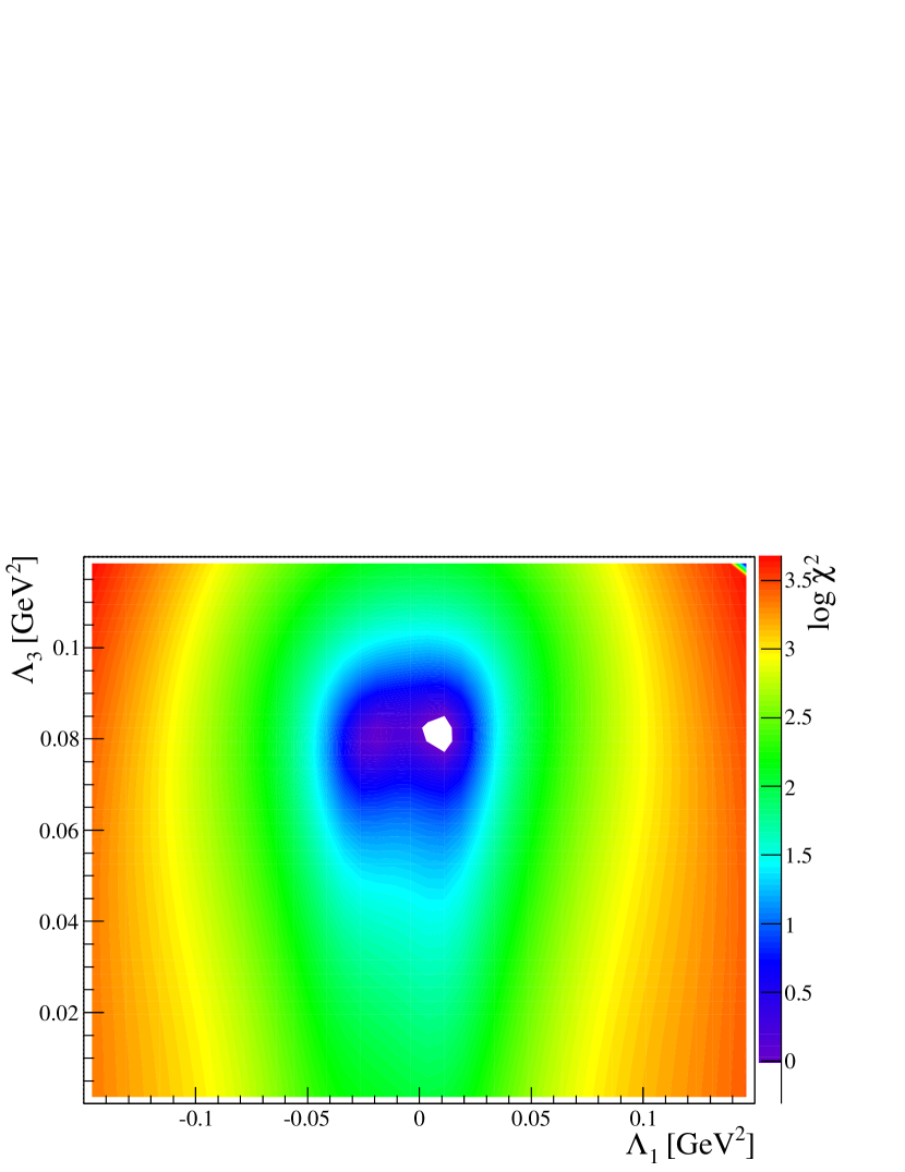
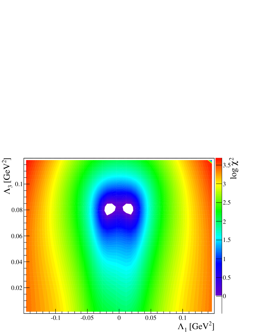
Figure 2: $\chi^{2}$ as a function of the BRpV parameters $\Lambda_{1}$ and $\Lambda_{3}$ for $\sin{\alpha}\approx 0.0695$ (left) and $\sin{\alpha}=0$ (right), keeping the rest of the parameters as indicated in Table 2.

Good solutions to neutrino observables are represented by the white region, corresponding to $\chi^{2}<1$. We see that the countours are not symmetric under a $\Lambda_{1}$ sign change. This is due to the $\chi^{2}$-term corresponding to the reactor angle in eq. (51), and can be understood from eq. (37). We see that the correction to the reactor angle due to a non diagonal charged lepton mass matrix is large because, in addition to the fact that $\sin\alpha\ll\cos\alpha$, we also have $|\Lambda_{2}|\gg|\Lambda_{1}|$ compensating the previous disbalance. Therefore, $\sin\theta_{13}$ is not symmetric under a change in the sign of $\Lambda_{1}$ unless it is accompanied by a corresponding change in the sign of $\Lambda_{2}$.

In order to see the effect of the diagonalization of the charged lepton mass matrix, we compare the same effect as before but now setting $\sin\alpha=0$, which is equivalent to a diagonal charged lepton mass matrix. This is done in Fig. 2-right, where we have the analogous countour plot for $\chi^{2}$. One sees that for the chosen point in parameter space, the allowed (white) region for the case $\sin{\alpha}\approx 0.0695$ (Fig. 2-left) is smaller than the corresponding region for the case $\sin{\alpha}=0$ (Fig. 2-right). This means that points in parameter space consistent with neutrino observables when the diagonalization of the charged lepton mass matrix is neglected, can actually be inconsistent when this diagonalization is taken into account. In addition, an approximated symmetry under the $\Lambda_{1}$ sign change is re-established in the case of $\sin{\alpha}=0$. This is because in this case $\sin^{2}\theta_{rea}$ is insensitive to this sign.

The previous conclusions are confirmed when we study separately the effect on $\chi^{2}$ from the neutrino angles. We remind the reader that the neutrino masses are not affected by the diagonalization matrix in the charged lepton sector, as we explained below eq. (35). In addition, the effect of the non-diagonal charged lepton matrix on the atmospheric angle is relatively small. The solar and reactor angles however get significant changes after the inclusion of charged lepton diagonalization effects. To show this we define,

$$\chi^{2}_{s2sol}=\left(\displaystyle{\frac{\sin^{2}{\theta_{sol}}-0,33}{0,07}}\right)^{2}\,,\qquad\chi^{2}_{s2rea}=\left(\displaystyle{\frac{\sin^{2}{\theta_{rea}}-0,018}{0,017}}\right)^{2}$$ (52)

which are the isolated contributions to $\chi^{2}$ from the solar and reactor angles respectively.

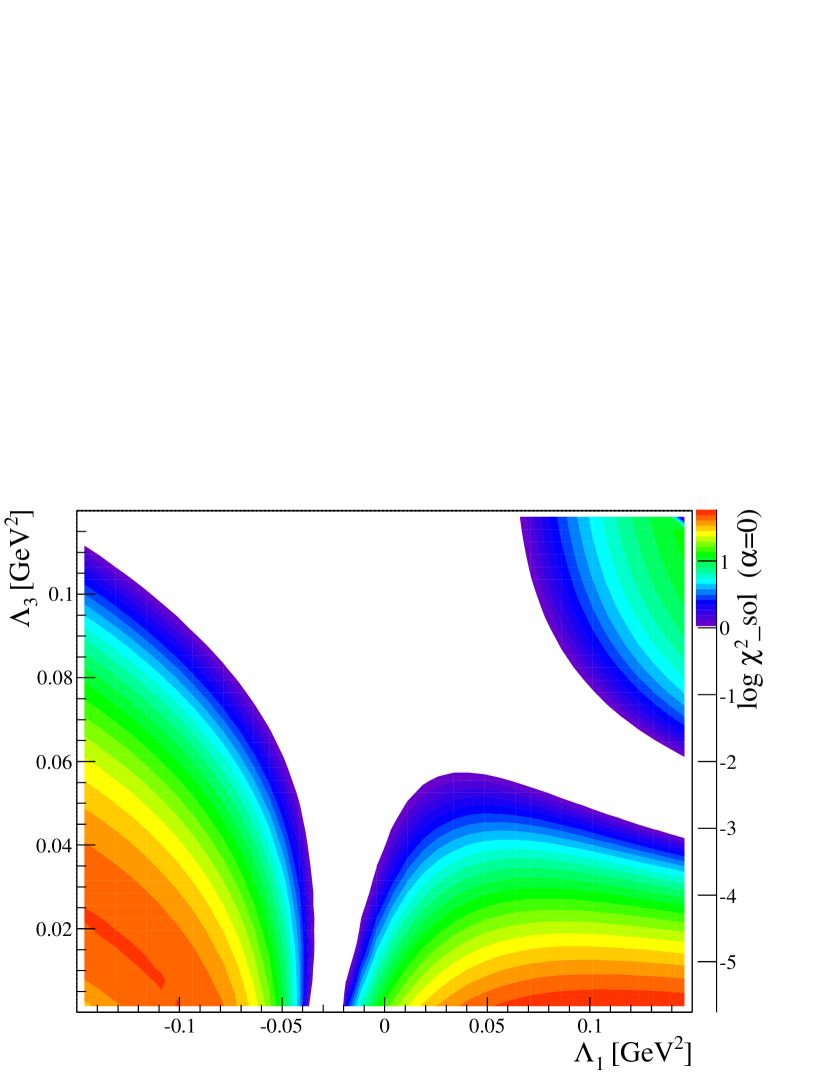
Figure 3: $\chi^{2}_{s2sol}$ as a function of the BRpV parameters $\Lambda_{1}$ and $\Lambda_{3}$ for $\sin{\alpha}\approx 0.0695$ (left) and $\sin{\alpha}=0$ (right), keeping the rest of the parameters as indicated in Table 2.

In Fig. 3 we have $\chi^{2}_{s2sol}$, with $\sin{\alpha}\approx 0.0695$ in the left frame and $\sin{\alpha}=0$ in the right one. We see important differences in the shape of the allowed region (white). Nevertheless the overall significance is decreased because the contribution from the solar angle to $\chi^{2}$ is relatively small.

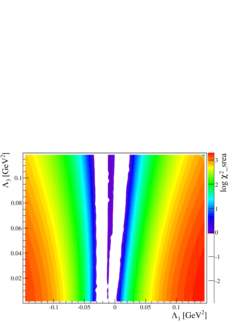
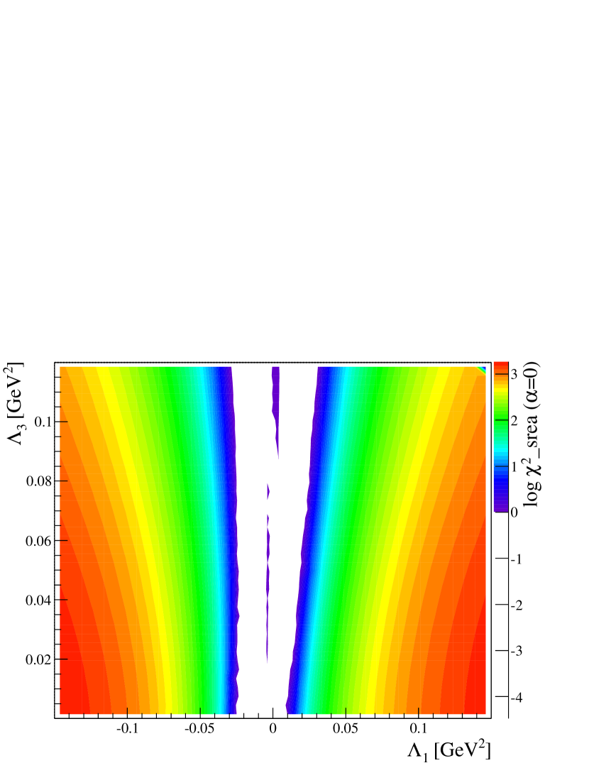
Figure 4: $\chi^{2}_{s2rea}$ as a function of the BRpV parameters $\Lambda_{1}$ and $\Lambda_{3}$ for $\sin{\alpha}\approx 0.0695$ (left) and $\sin{\alpha}=0$ (right), keeping the rest of the parameters as indicated in Table 2.

On the other hand, in Fig. 4 we have $\chi^{2}_{s2rea}$ with an analogous difference between left and right frames. The shift in the allowed region from left ($\sin{\alpha}\approx 0.0695$) to right ($\sin{\alpha}=0$) is much smaller than in the solar angle case, but the numerical contribution to $\chi^{2}$ from the reactor angle is much larger, making the reactor angle the most decisive factor in the influence of the diagonalization of the charged lepton mass matrix. We also mention that the prediction in Diaz:2009yz that $\mu_{g}={\mathcal{O}}(0.01)$ eV is not affected by the scenario where the charged lepton mass matrix is not diagonal, since $\mu_{g}$ is in first approximation restricted only by mass differences.

VII.2 Partial Split SUSY

In PSS the parameter space consists of, first, the supersymmetric parameters Bino mass $M_{1}$, Wino mass $M_{2}$, Higgsino mass $\mu$, $\tan{\beta}$, and Higgs masses $m_{h}$ and $m_{A}$, which define the constants $A$ and $C$ in eq. (44); second, the BRpV parameters $\Lambda_{i}$ and $\epsilon_{i}$; and third, the charged lepton Yukawa parameters $E$, $F$, and $D$, which define the angles $\sin{\alpha}^{\prime}$ and $\sin{\theta}^{\prime}$ in (19).

As we did for the previous model, we perform a scan over parameter space and look for solutions with predictions on neutrino observables compatible with experimental data, represented by the value of $\chi^{2}<1$ as given in eq. (51). A working scenario satisfying this criteria is given in Table 4. The effect of the first 6 parameters is in the values of $A$ and $C$ which enter in the neutrino mass matrix. The scale $Q$ is chosen such that there is no mixing term between $\Lambda$ and $\epsilon$. The scenario is completed with the values of the BRpV parameters $\Lambda_{i}$ and $\epsilon_{i}$. In Table 4 we have the predictions for the neutrino observables in this model, which gives a value of $\chi^{2}=0.88$.

SUSY Parameters	Value	Scanned Range	Units
$M_{1}$	$119$	$[40,500]$	GeV
$M_{2}$	$339$	$[80,100]$	GeV
$|\mu|$	$456$	$[0,1000]$	GeV
$\tan{\beta}$	$5.71$	$[2,50]$	-
$m_{h}$	$130$	$[114,140]$	GeV
$m_{A}$	$1963$	$[500,6000]$	GeV
$A$	$-2.73$	-	${\mathrm{eV}}/{\mathrm{GeV}}^{4}$
$C$	$0.282$	-	${\mathrm{eV}}/{\mathrm{GeV}}^{2}$
$Q$	$1048$	-	GeV
BRpV Parameters	Value	Scanned Range	Units
$\Lambda_{1}$	$0.0317$	$[-1,1]$	$\mbox{GeV}^{2}$
$\Lambda_{2}$	$-0.0022$	$[-1,1]$	$\mbox{GeV}^{2}$
$\Lambda_{3}$	$0.0738$	$[-1,1]$	$\mbox{GeV}^{2}$
$\epsilon_{1}$	$0.034$	$[-1,1]$	GeV
$\epsilon_{2}$	$0.264$	$[-1,1]$	GeV
$\epsilon_{3}$	$0.372$	$[-1,1]$	GeV

Table 3: Chosen values for PSS. This values gives $\chi^{2}=0.88$.

Observable	Solution	Units
$\Delta m_{atm}^{2}$	$2.43\times 10^{-3}$	$\mbox{eV}^{2}$
$\Delta m_{sol}^{2}$	$7.66\times 10^{-5}$	$\mbox{eV}^{2}$
$\sin^{2}{\theta}_{atm}$	$0.495$	-
$\sin^{2}{\theta}_{sol}$	$0.323$	-
$\sin^{2}{\theta}_{rea}$	$0.0026$	-

Table 4: PSS predictions for neutrino observables given the values in Table 4.

Similarly to the previous model, in Fig. 5-left we have the logarithm of $\chi^{2}$ as contour regions in the $\epsilon_{3}$-$\epsilon_{1}$ plane, with all the other parameters fixed at their values in Table 4, plus $\sin\alpha^{\prime}=0.070$ and $\sin\theta^{\prime}=0.036$. The white region corresponds to $\chi^{2}<1$, i.e. points that satisfy the experimental constraints. Neglecting the effects of the diagonalization of the charged lepton mass matrix corresponds to set $\sin\alpha^{\prime}=\sin\theta^{\prime}=0$, and when this is done we find $\chi^{2}=2.81$, meaning that a good point could have been missed if the charged lepton mass matrix diagonalization had not been taken into account. This can be seen graphically from Fig. 5-right which is the analogous to the previous figure but neglecting the charged lepton mass matrix diagonalization.

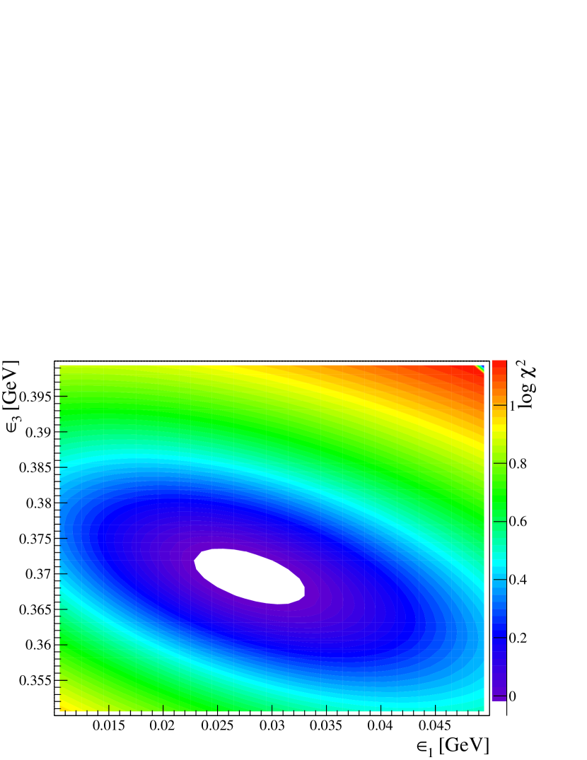
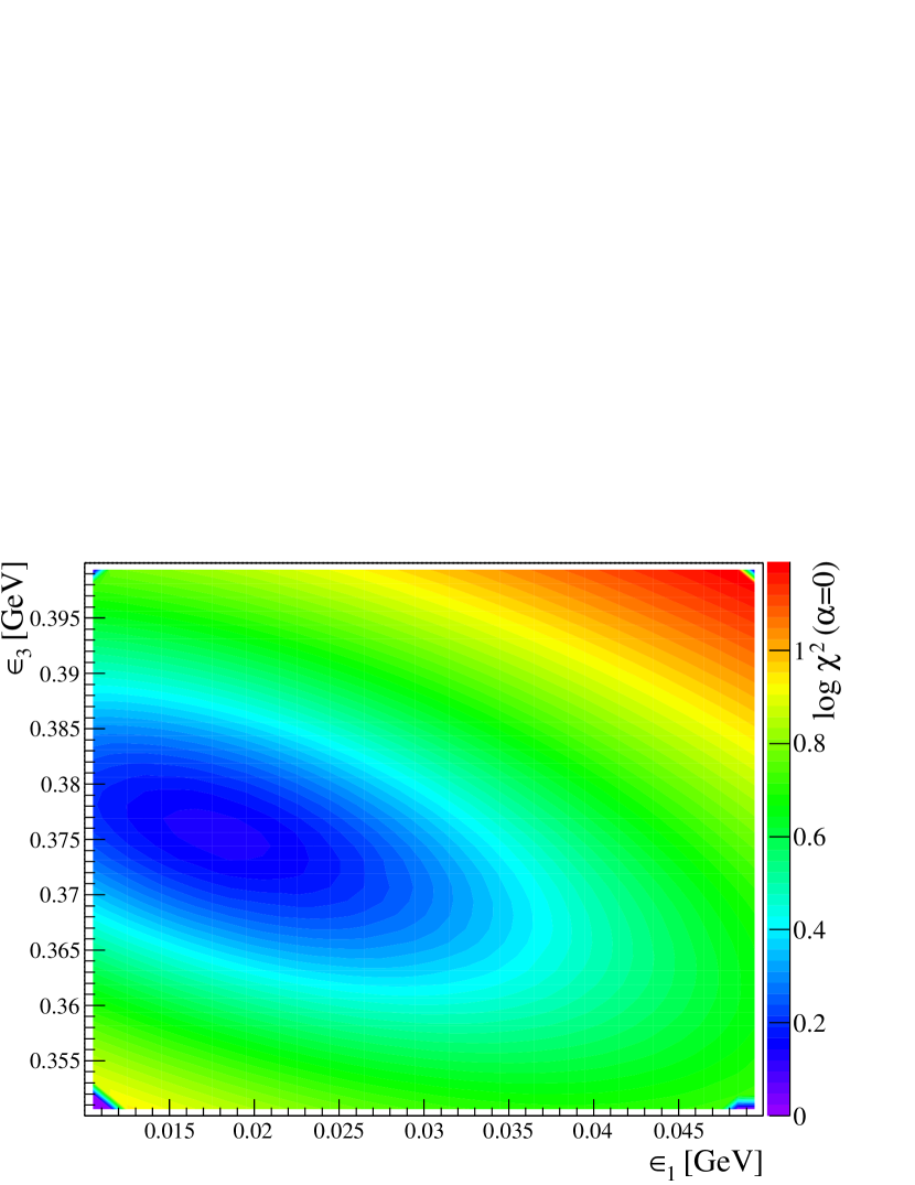
Figure 5: $\chi^{2}$ in dependence of $\epsilon_{2}$ and $\epsilon_{3}$, while the other parameters are fixed around the central value from table4. On the left hand side $\sin\alpha^{\prime}=0.070$ and $\sin\theta^{\prime}=0.036$ was used, while on the right hand side a diagonal charged lepton matrix was used.

It is useful to study the individual dependence of the neutrino angles on the charged lepton rotation matrix angles $\alpha^{\prime}$ and $\theta^{\prime}$. In Fig. 6 we have solar angle (left) and reactor angle (right) as a function of $\sin\alpha^{\prime}$ for three different values of $\sin\theta^{\prime}$.

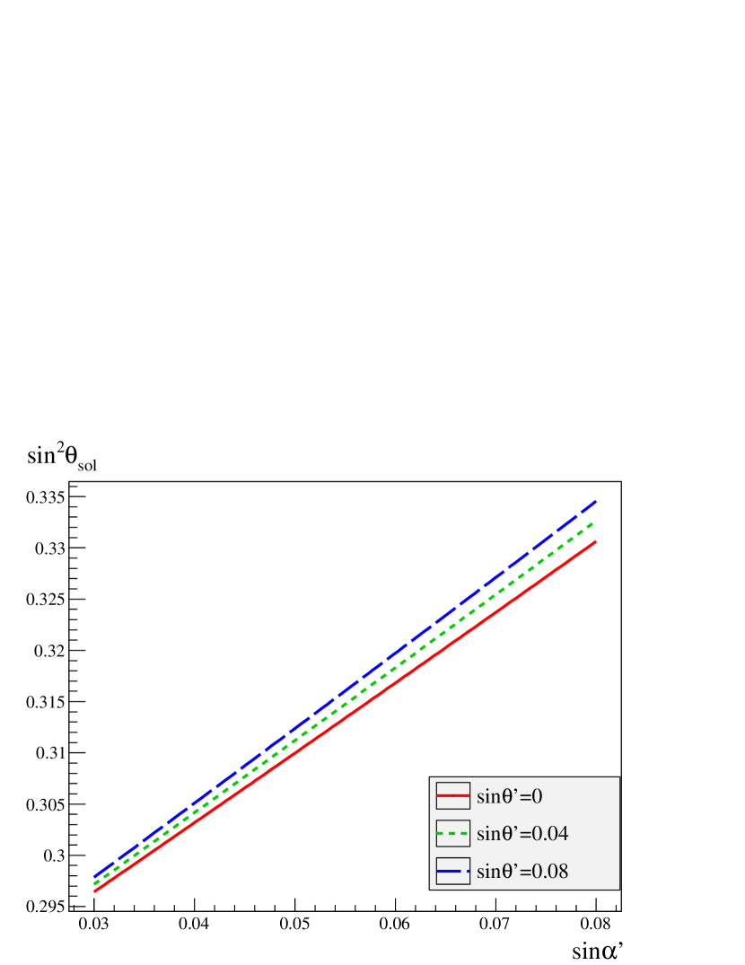
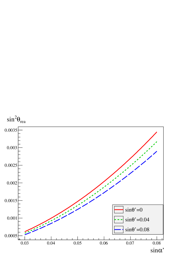
Figure 6: $\sin^{2}{\theta}_{sol}$ and $\sin^{2}{\theta}_{rea}$ dependence on $\sin{\alpha}^{\prime}$ for different values of $\sin{\theta}^{\prime}$. The other parameters are fixed around the central values in table 4.

In both cases the dependence on $\sin\alpha^{\prime}$ is stronger that the dependence on $\sin\theta^{\prime}$, as can be noticed from eqs. (50), where we see that the solar and reactor angles depend at first order only on $\sin\alpha^{\prime}$, and a dependency on $\sin\theta^{\prime}$ appears only at second order. Although the dependency of the solar angle on $\sin\alpha^{\prime}$ is strong, it variation on the chosen range for $\sin\alpha^{\prime}$ maintains the solar angle within its $3\sigma$ experimental region. On the contrary, the reactor angle being also very sensitive to $\sin\alpha^{\prime}$ it can escape from below the experimental widow, while keeping its value well below the upper $3\sigma$ bound. Therefore, a lower bound on the reactor angle already constraints the model.

In Fig. 7 we have a similar plot for the dependence of the atmospheric angle on $\sin{\theta}^{\prime}$ for three different values of $\sin{\alpha}^{\prime}$. As opposed to the previous cases, for the atmospheric angle the dependence is stronger on $\sin{\theta}^{\prime}$ rather than on $\sin{\alpha}^{\prime}$.

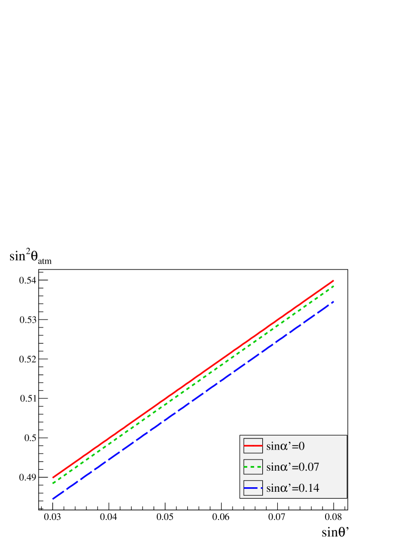
Figure 7: $\sin^{2}{\theta}_{atm}$ dependence on $\sin{\theta}^{\prime}$ for different values of $\sin{\alpha}^{\prime}$. The other parameters are fixed around the central values in table 4.

From eq. (50) we see that despite the fact that $\tan\theta_{23}$ depends at first order on both angles, $\sin{\alpha}^{\prime}$ is multiplied by the reactor angle and makes its influence much smaller. In any case, over the chosen range for $\sin{\theta}^{\prime}$, the atmospheric angle does not leave the $3\sigma$ experimental window.

In a related numerical analysis we plot in Fig. 8 the allowed region (defined by $\chi^{2}<1$) in the $\sin{\theta}^{\prime}$-$\sin{\alpha}^{\prime}$ plane, with the effect of the different neutrino angle $3\sigma$ bounds shown as solid lines.

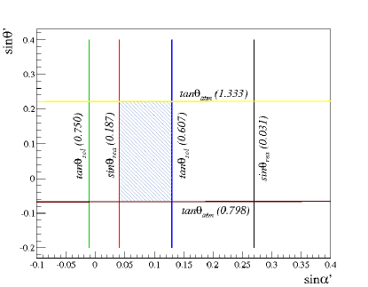
Figure 8: Range of $\sin\theta^{\prime}$ and $\sin\alpha^{\prime}$ that gives $\chi^{2}<1$, for the scenario given in Table 4.

Here we confirm that the atmospheric angle restricts the values of $\sin{\theta}^{\prime}$, while the solar and reactor angles restricts the values of $\sin{\alpha}^{\prime}$. The typical value for the charged lepton mixing angles in the Giudice ansatz are $\sin{\theta}^{\prime}=0.036$ and $\sin{\alpha}^{\prime}=0.07$, and $\theta^{\prime}$ will start to be probed if the error in the atmospheric angle diminishes by a few times. On the other hand the value of $\alpha^{\prime}$ can be probed with an improvement on the lower bound of the reactor angle, and with an improvement on the upper bound of the solar angle.

VIII Summary

Usually the Yukawa matrix of the charged leptons is assumed to be diagonal. However, it is known that this does not necessarily have to be the case. In order to see how this assumptions affect neutrino observables we studied the impact of a non-diagonal charged lepton Yukawa matrix on the neutrino sector of split supersymmetric models. This was done by using two different ansätze for the charged lepton matrix. It was found that the mass differences between the different neutrino species are effectively insensitive to the charged lepton sector. This confirms the usual assumption of a diagonal charged lepton matrix with this respect. However, when studying the neutrino mixing angles it was found that the form of the mass matrix of the charged leptons indeed can provoke significant changes in the observables. We found that especially the solar and reactor mixing angles are sensible to this generalization, whereas the atmospheric angle shows a somewhat weaker dependence. Thus, it has been shown that the usual assumption of a diagonal mass matrix for charged leptons, can lead to important mistakes in the interpretation of experimental data. In other words, within a given model a parameter point that agrees with the experimental neutrino data in the context of a diagonal charged lepton matrix, is likely to disagree with the data in the context of a non-diagonal charged lepton matrix or viceversa.

- (1) R. Barbier et al., Phys. Rept. 420, 1 (2005) [arXiv:hep-ph/0406039]; H. K. Dreiner, arXiv:hep-ph/9707435.
- (2) R. Hempfling, Nucl. Phys. B 478, 3 (1996) [arXiv:hep-ph/9511288]; M. Drees, S. Pakvasa, X. Tata and T. ter Veldhuis, Phys. Rev. D 57, 5335 (1998) [arXiv:hep-ph/9712392]; E. J. Chun, S. K. Kang, C. W. Kim and U. W. Lee, Nucl. Phys. B 544, 89 (1999) [arXiv:hep-ph/9807327]; Y. Grossman and S. Rakshit, Phys. Rev. D 69, 093002 (2004) [arXiv:hep-ph/0311310]; S. Davidson and M. Losada, JHEP 0005, 021 (2000) [arXiv:hep-ph/0005080];
- (3) M. A. Diaz, S. G. Saenz and B. Koch, Phys. Rev. D 84, 055007 (2011) [arXiv:1106.0308 [hep-ph]].
- (4) M. A. Diaz, M. Hirsch, W. Porod, J. C. Romao and J. W. F. Valle, Phys. Rev. D 68, 013009 (2003) [Erratum-ibid. D 71, 059904 (2005)] [hep-ph/0302021].
- (5) M. A. Diaz, B. Koch and B. Panes, Phys. Rev. D 79, 113009 (2009) [arXiv:0902.1720 [hep-ph]].
- (6) M. A. Diaz, F. Garay, B. Koch, Phys. Rev. D80, 113005 (2009). [arXiv:0910.2987 [hep-ph]].
- (7) D. Restrepo, M. Taoso, J. W. F. Valle and O. Zapata, arXiv:1109.0512 [hep-ph].
- (8) H. Georgi, C. Jarlskog, Phys. Lett. B86, 297-300 (1979).
- (9) S. Dimopoulos, L. J. Hall and S. Raby, Phys. Rev. D 45 (1992) 4192.
- (10) W. Krolikowski, hep-ph/0509184.
- (11) K. Nakamura et al. [ Particle Data Group Collaboration ], J. Phys. G G37, 075021 (2010).
- (12) G. F. Giudice, Mod. Phys. Lett. A7, 2429-2436 (1992). [hep-ph/9204215].
- (13) H. K. Dreiner, G. K. Leontaris, S. Lola, G. G. Ross and C. Scheich, Nucl. Phys. B 436, 461 (1995) [hep-ph/9409369].
- (14) G. K. Leontaris, S. Lola, C. Scheich and J. D. Vergados, Phys. Rev. D 53, 6381 (1996) [hep-ph/9509351].
- (15) S. K. Kang and C. S. Kim, Phys. Rev. D 63, 113010 (2001) [hep-ph/0012046].
- (16) N. Arkani-Hamed and S. Dimopoulos, JHEP 0506, 073 (2005) [arXiv:hep-th/0405159]; G. F. Giudice and A. Romanino, Nucl. Phys. B 699, 65 (2004) [Erratum-ibid. B 706, 65 (2005)] [arXiv:hep-ph/0406088].
- (17) M. A. Diaz, P. Fileviez Perez and C. Mora, Phys. Rev. D 79, 013005 (2009) [arXiv:hep-ph/0605285].
- (18) S. Davidson, M. Losada, Phys. Rev. D65, 075025 (2002). [hep-ph/0010325]; Y. Grossman and S. Rakshit, “Neutrino masses in R-parity violating supersymmetric models,” Phys. Rev. D 69, 093002 (2004) [arXiv:hep-ph/0311310].
- (19) V. Berezinsky, M. Narayan, F. Vissani, JHEP 0504, 009 (2005). [hep-ph/0401029].
- (20) R. Sundrum, JHEP 1101, 062 (2011) [arXiv:0909.5430 [hep-th]].
- (21) S. Weinberg, Phys. Rev. Lett. 43, 1566 (1979).
- (22) M. Hirsch, H. V. Klapdor-Kleingrothaus and S. G. Kovalenko, Phys. Lett. B 398, 311 (1997) [arXiv:hep-ph/9701253].
- (23) M. Maltoni, T. Schwetz, M. A. Tortola and J. W. F. Valle, New J. Phys. 6 122 (2004) [arXiv:hep-ph/0405172].
- (24) T. Schwetz, M. Tortola and J. W. F. Valle, New J. Phys. 13, 063004 (2011) [arXiv:1103.0734 [hep-ph]].
- (25) T. Schwetz, M. Tortola and J. W. F. Valle, New J. Phys. 13, 109401 (2011) [arXiv:1108.1376 [hep-ph]].