Finding proto-spectroscopic binaries

The formation of spectroscopic binaries (SB) may be a natural byproduct of star formation. The early dynamical evolution of multiple stellar systems after the initial fragmentation of molecular clouds leaves characteristic imprints on the properties of young, multiple stars. The discovery and the characterization of the youngest SB will allow us to infer the mechanisms and timescales involved in their formation. Our work aims to find spectroscopic companions around young stellar objects (YSO). We present a near-IR high-resolution (R $\sim$ 60000) multi-epoch radial velocity survey of 7 YSO in the star forming region (SFR) $\rho$ Ophiuchus. The radial velocities of each source were derived using a two-dimensional cross-correlation function, using the zero-point established by the Earth’s atmosphere as reference. More than 14 spectral lines in the CO $\Delta\nu$ = (0-2) bandhead window were used in the cross-correlation against LTE atmospheric models to compute the final results. We found that the spectra of the protostars in our sample agree well with the predicted stellar photospheric profiles, indicating that the radial velocities derived are indeed of stellar nature. Three of the targets analyzed exhibit large radial velocity variations during the three observation epochs. These objects - pending further confirmation and orbital characteristics - may become the first evidence for proto-spectroscopic binaries, and will provide important constraints on their formation. Our preliminary binary fraction (BF) of $\sim$71% (when merging our results with those of previous studies) is in line with the notion that multiplicity is very high at young ages and therefore a byproduct of star formation.

1 Introduction

Since the early twenties that there is growing evidence that multiple stars may be the rule and not the exception. This conception is more recentlt supported by observations of Duquennoy & Mayor (1991) who found that the stellar multiplicity among main sequence (MS) stars in the solar neighborhood may be as high as $\sim$ 60%. Since then, more refined surveys probed the dependencies of the properties of stellar systems on physical parameters like age, mass, separation, and environment. These observations are highly relevant, because there is still no comprehensive theory that explains the properties of multiple stars and their relation to star formation. Recently, Raghavan et al. (2010) confirmed that stellar multiplicity decreases with stellar mass (or later spectral type) in the vicinity of the Sun, a finding that was already suggested earlier (e.g. Siegler et al., 2005; Lada, 2006). Because the stellar population in the solar neighborhood is dominated by late-type M-stars, this implies that about half of the solar-like main sequence stars in the solar neighborhood occur in multiple systems.
It is likely that the multiplicity rate of stars is established in the early phases of star formation or during the dynamical evolution that occurs afterwards (Goodwin et al., 2004; Delgado-Donate et al., 2004; Bate, 2009). And it is plausible that both initial and environmental conditions constrain multiple star formation, and play a vital role in explaining their evolution over time, and their relation to the observed MS stellar multiplicity (Mathieu et al., 2000; Sterzik et al., 2003; Connelley et al., 2008; Köhler et al., 2008; Kaczmarek et al., 2011). It is therefore essential to probe the stellar multiplicity as early as possible, to gain a full understanding of the formation and the dynamical evolution of multiple systems.
Ghez et al. (1993); Leinert et al. (1993); Simon et al. (1995); Patience et al. (2002); Beck et al. (2003) and Duchêne et al. (2004, 2007) all noted differences in the BF of pre-main-sequence (PMS) stars in different SFRs. In particular, the multiplicity of T Tauri stars with ages $\lesssim$ 10⁶ yrs, appears to be higher by a factor of 2 in less dense regions such as Taurus compared to denser SFR such as Ophiuchus (e.g. Simon et al., 1995; Beck et al., 2003; Ratzka et al., 2005) or the field (Patience et al., 2002; Duchêne et al., 2004). Toward even younger ages, radio continuum (e.g. Reipurth et al., 2004) and near- and mid- Infrared (IR) (Barsony et al., 2005; Haisch et al., 2002, 2004, 2006) investigations found additional evidence for an even higher multiplicity among Class I and Flat-spectrum ($\sim$ 2 - 5 x 10⁵ yrs) protostars.
On the other hand, Maury et al. (2010) failed to detect companions in a small sample of 5 protostars at separations 50 <$a$ <5000 AU ($a$ being the semimajor axis) in a millimeter study of self-embedded, young (Class 0) objects ($\sim$ 10⁴ - 10⁵ yrs). Taken together with the observations of Looney et al. (2000), the authors argue that multiplicity in the separation ranges from 100 to 600 AU would only be defined in a later stage of star formation (namely after the Class 0 phase) and that early multiplicity in pristine systems may not be as ubiquitous and primeval.
However, all multiplicity studies in the earliest phases of stellar evolution are plagued with relatively small number statistics. In particular, very little is known about companions of embedded protostars at the sub-AU separation scales, a regime impossible to address with conventional imaging techniques. Spectroscopic Binaries (SB) may provide additional important constraints on the star-formation mechanism itself. Tokovinin & Smekhov (2002) and Tokovinin et al. (2006) estimated the SB frequency in MS stars and inferred that 65% of their sample of 165 spectroscopic binaries were members of higher order multiple systems, often found in a hierarchical configuration. Remarkably, the frequency of SB in multiple systems strongly depends on the orbital period of the SB: 96 of the SBs with orbital periods shorther than 3 days are in multiple systems, while this rate drops to 30% for SBs with orbital periods longer than 13 days. The higher frequency of spectroscopic system within triple or higher order systems suggests an imprint of the formation mechanism itself. Spectroscopic pairs may have lost their orbital angular momentum owing to the presence of a third body that interacts with the inner binary via Kozai cycles and tidal friction (Kozai, 1962; Sterzik et al., 2005; Fabrycky & Tremaine, 2007). This interaction has the effect of tightening the spectroscopic binary orbit, while the tertiary would eventually be evacuated to an outer region of the system. The SB may therefore hold an important fossil record of (prevailing) initial conditions during their formation. However, this scenario is not conclusive by itself, and it is not clear at which evolutionary stage this process operates efficiently. Observations are required to better constrain the detailed mechanisms of how tight binaries are formed at very young ages.
The first successful PMS SB detections were performed by Herbig (1977); Hartmann et al. (1986); Mathieu et al. (1989) and Mathieu (1994) in the Taurus and Ophiuchus SFRs with a radial velocity precision limited to $\sim$1kms^-1 by optical high-resolution spectroscopy. Since then, improving instrumental capabilities and better radial velocity precision allowed to address PMS sources and the lower mass regimes (e.g. Melo, 2003; Covey et al., 2006; Kurosawa et al., 2006; Joergens, 2006, 2008; Prato, 2007). Only recently, infrared (IR) high-resolution spectroscopy allowed the search for SB among the youngest, embedded PMS and the very low mass stars (e.g. Prato, 2007; Blake et al., 2007, 2010; Figueira et al., 2010b; Rice et al., 2010; Crockett et al., 2011). In particular (Figueira et al., 2010b; Blake et al., 2010; Crockett et al., 2011) reached a precision of less than 50 ms^-1 in PMS stars and very low mass stars. Even the planetary mass regime may be in reach using high-stability, high-precision IR spectroscopy.
Our own work aims to find SBs in a sample of 38 Class I/ II protostars in the SFR $\rho$ Ophiuchus. We performed a high-resolution IR spectroscopic survey to derive precision radial velocities (RV) using the NIR spectrograph CRIRES at the VLT (Kaeufl et al., 2004). We describe our sample, the data analysis methodology and results in Sect. 2. Sect. 3 discusses the RV derived in the context of the $\rho$ Ophiuchus SFR and its implications on the formation of SB at very young ages in general. In Sect. 4. we draw our conclusions.

Figure 1: Process of telluric signature removal in DET4. The extracted nodded spectra of GSS26 (A) is divided by the spectrum of the telluric standard stars with the same exposure time and observed closest in time (same airmass) (B). Lower panel exhibits ’cleaned’ nodded spectrum (C).

2 Observational aspects and analysis

2.1 Observations and data reduction

The arrival of CRIRES (Kaeufl et al., 2004), a high-resolution near- and mid-IR spectrograph mounted on Antu at the Paranal Observatory allowed for the first time to acquire radial velocity measurement precision of a few ms^-1 level in this wavelength window. CRIRES has opened the possibility to look for (low-mass) spectroscopic companions around young stars that are otherwise too faint to be observed in the optical because of the extinction caused by circumstellar material. It also entails improved ability to detect dimmer companions to optical bright primaries through more favorable flux ratios (e.g. Mace et al., 2009).

This study intends to take advantage of CRIRES to measure radial velocities in a sample of Class I/II protostars whose multiplicity at larger scales has already been determined by imaging techniques. The main purpose consists in detecting radial velocity variations caused by potential close companions and to compare the overall multiplicity frequency in embedded sources as a function of separation with those observed for T-Tauri and MS stars from the sub-AU to a thousand AU scale.

To this aim, a sample of 38 Class I/ Flat spectrum objects was selected from the near- and mid-Infrared multiplicity studies of Haisch et al. (2002, 2004, 2006). The main selection criteria was the apparent $K$-band magnitude of the targets. As a compromise between the telescope time required to reach the desired S/R and the size of the sample, this limit was set at $K<11$. In addition, we selected proto-stars from 3 different SFRs to allow us a preliminary investigation of the role of the environment in our measured spectroscopic binary fraction.

In CRIRES the incoming light enters the instrument and is first directed into a pre-disperser, after which it is dispersed in a 31.6 lines/mm echelle grating. It delivers high-resolution spectra (up to $\sim$100 000 with the a 0.2”-slit) in the 960 - 5200 nm interval in wavelengths windows of $\sim\lambda$/70. The observed light is finally projected into four Aladdin III detectors (4096 $\times$ 512 pixel) separated by $\sim$ 250 pix. The combination of the size of the detectors and the high resolution of the instrument limits the wavelength coverage of CRIRES, which is considerably smaller than that of other spectrographs. Therefore the first task was to find out the best set-up among the 200 available to obtain the most accurate radial velocities as a function of the signal-to-noise ratio.
In order to estimate the S/R necessary to reach the required precision, we investigated the amount of information (i.e., number of available spectral lines and their intensity) by simulating all CRIRES set-ups as described in Figueira et al. (2010b). In a nutshell, the estimated error on the radial velocity is given by $\epsilon(V_{r})\propto R\leavevmode\nobreak\ [(S/R)<I>n^{1/2}_{l}]^{-1}$, where R is the instrumental resolution, $\epsilon$ is the photon noise error, S/R is the signal-to-noise ratio, $<I>$ is the average depth of absorption lines, and $n_{l}$ is the number of lines entering in the computation of the CCF. In order to simulate all CRIRES set-ups, we used the IR solar spectrum obtained with the Fourier Transform Spectrograph provided by the NOAO (Wallace et al., 1993). This solar spectrum was convolved with a Gaussian function and trimmed to match the resolution and wavelength coverage of the various CRIRES set-ups (for details see Figueira et al., 2010b). Assuming that only stellar lines deeper than a certain threshold contribute to the CCF, the above expression was applied to all CRIRES simulated spectra and the quantity $\epsilon(Vr)/S/R$ was derived as a function of the set-up. This ratio allowed us to compare the radial velocity error (in a relative way) among the set-ups and to choose the most suitable one. A few set-ups were identified in the H- and K-band (see Fig. 1 of Figueira et al., 2010b). Because of the unknown degree of obscuration of our sample, we selected the K-band set-up.
To derive the absolute error and therefore be able to transform the ratio $\epsilon(Vr)/S/R$ into exposure times, we had to know the absolute error on $V_{r}$ as a function of the S/R for one set-up. Our exposures times were then computed assuming that an S/R of 20-30 in the setting chosen here would give a 150m/s error for the set-up former 24/-1/i setting. In practice, this estimate turned out to be too optimistic. As a consequence, exposure times for several targets were underestimated. Accordingly, we obtained 15 protostars with robust RV measurements from the original 38 stars proposed and only 7 sources with multiple RV measurements at sufficient S/R. This paper focus on these 7 multi-epoch targets from the $\rho$ Ophiuchus SFR, for which we detected photospheric absorption features. In Table LABEL:table:1 we present the properties of the full sample. An assessment of the evolutionary status of each sources is presented in the column SED of Table LABEL:table:1. It follows the usual YSO classification based on the change of the slope of the SED as a function of age. Rising SEDs with positive slopes toward mid-IR usually depict the presence of protostellar envelopes that are generally more massive than the protostar. These protostellar envelopes tend to disappear in the subsequent phases of evolution, namely the Class I phase. As a consequence, the SED slope flattens (flat-spectrum sources) and then becomes negative towards the Class II or T-Tauri phase. (e.g. Motte & André, 2001).
Our sample was observed between April 2008 and February 2009 with a set-up covering a wavelength range of 2254.2 to 2304.7 nm. The center wavelength reference in detector3 (DET3) was $\lambda$2287.1 nm. The CO (2-0) bandhead at 2293.5nm was registered on detector 4 (DET4). Owing to the lack of reference stars close to our science targets, our observations were carried out in the seeing-limited mode. Observations were collected under good seeing ($\sim$ 0.8”) in 2 nodding cycles (i.e., 4 total independent exposures) , with a 0.3” wide slit allowing a resolution of $\sim$ 60,000 which we found to be the best compromise between the amount of flux entering the spectrograph and the ability to resolve the lines of the object and those from the atmosphere. Final S/N ratios given in Table LABEL:table:1 were computed on small featureless regions.
The approximate range of masses of our 7 protostellar targets was taken from Natta et al. (2006) and assumed to be within the interval from 0.18 $M_{\odot}$ to 1.4 $M_{\odot}$. Assuming that semi-amplitudes of 500m/s can be measured at a 3$\sigma$ level, we are able to detect companions ranging from several jupiter masses with periods of one or a few weeks to equal-mass companions (from brown dwarfs to solar-type stars) with periods of several years. A more detailed study of the detectability rate similar to the one performed by Melo (2003) will be carried out at the end of the survey.
In addition to the protostellar data we also collected spectra of telluric standard stars (featureless early-type B stars) observed with the same airmass and instrumental setup as our science targets. Multi-epoch spectra of 3 radial velocity standard stars were collected during the timespan of our observations in order to study the precision of our RV measurements.
Data were reduced using an optimized IRAF-based pipeline to ensure a uniform and homogeneous reduction for all targets in the different epochs. The reduction steps in our pipeline were: 1) correction for CRIRES nonlinearity using ESO on-line coefficients and construction of bad-pixel masks, 2) dark-current subtraction from the flatfield images and collapsing into a master flat, 3) division of science spectra by these final flatfield images, 4) subtraction of opposing nodded spectra for dark-current removal, 5) optimal extraction using the Horne (1986) algorithm, 6) telluric signature removal by dividing each extracted spectrum by the spectrum of the telluric STD stars with the same exposure time and observed closest in time (same airmass) (Fig. 1).
The position of the CCF peak strongly depends on the average center of all stellar lines used to computed the CCF. Because telluric removal could have changed the final line shapes, it is essential to find the most similar and adequate telluric spectra so as not to change the protostellar line shapes fundamentally. A test was carried out to assess the impact of the use of different observed telluric spectra in the derived RVs. First, we performed for a specific date telluric line removal with the observed telluric standard and the combined science spectra of protostars where no stellar signal was detected (i.e., only the atmospheric lines are imprinted in the data). The main conclusion was that small fluctuations ($\lesssim$ 50ms^-1) on the final RV could indeed be detected. These discrepancies were found in tellurics that were observed $\geq$2 hours after the science target. We found no relevant differences in the final RV when the telluric removal was performed with tellurics observed within that time difference. We conclude that telluric removal as explained here has no major impact on the final RV.

Figure 2: Extracted spectra of our Class-I stars as observed in Detector 4. The data shown here were smoothed for clarity, continuum-normalized and Doppler-corrected to a null radial velocity.

The extracted spectra were wavelength-calibrated using telluric absorption lines. The use of telluric features to build a wavelength solution is now a well-documented technique (Caccin et al., 1985; Blake et al., 2007; Figueira et al., 2010b; Blake et al., 2010; Crockett et al., 2011) and it is highly convenient when gas cells are not available as was the case of CRIRES at the time of the observations. We refer the reader to (e.g. Figueira et al., 2010a) or Blake et al. (2010) for an extensive explanation of the robustness of this technique. The study of Figueira et al. (2010a), in particular, showed that O2 atmospheric lines can be stable down to 10 m/s over long periods of time (6 years).
Basically, wavelength solution construction consists in finding and fitting (in each observed spectrum) the center of telluric lines with low-order polynomials to match their theoretical value as given by online databases. In our particular setting, we took advantage of the wealth of CH₄ atmospheric telluric lines to build suitable wavelength solutions for each extracted spectrum. This set of CH₄ lines has already been used in previous studies and was shown to deliver precise RVs in very low-mass stars and in brown dwarves (Blake et al., 2007, 2010). The reference wavelength of each spectral line was taken from the HITRAN database with a typical accuracy $\lesssim$ 50ms^-1, which is well-suited to our purposes, giving the radial velocity amplitudes expected by the presence of stellar companions. Spectral features of protostars are known to be considerably broader than MS stars or even class-II stars (Greene & Lada, 1997; Doppmann et al., 2005), because of their typically high vsini. For this reason, we expected to find a high level of blending between spectral features of telluric and stellar origin that could introduce significant systematic errors when building the wavelength solution or determining the RV measurements. To minimize possible systematic errors arising from the overlap of the telluric with the stellar signal, we combined all nodded images from each target’s observation into a single frame for building the wavelength solutions. This procedure considerably improved the S/N of the final spectra, which is therefore ensured a better identification and fitting of telluric lines and their theoretical centers. This steps assumes that the spectral characteristics of the atmosphere did not vary between nodded positions (i.e., in time-scales of $\leq$4 min in K-band).

2.2 Data analysis

The RVs in this study were derived using a slightly different version of the Figueira et al. (2010b) pipeline, a two-dimensional (2D) cross-correlation function (CCF) based on TODCOR (Mazeh & Zucker, 1992). The pipeline of Figueira et al. (2010b) was specifically designed to deliver the RV of the target relative to the zero-point established by the Earth’s atmosphere.
In a 2D cross-correlation using atmospheric lines as a reference, the RV of the atmosphere (RV_sky) and the RV of the star (RV_star) were obtained from the same spectrum by cross-correlating the observed spectrum with a combination of two CORAVEL-type masks (i.e., the absorption lines are represented by box-shaped lines, see Baranne et al., 1996), one mask containing the telluric lines and another the stellar lines. As mentioned in the previous section, the lines present in the atmospheric mask use the HITRAN wavelengths as reference. The stellar masks were built using the synthetic spectra of PHOENIX for stellar type G8V, K2V, K5V, M1 and M6. The width of the box-shaped line was set by convolving the synthetic spectra with Gray’s rotational profiles (Gray, 1992) with the rotational velocities chosen to adjust the line width of the observed spectra. The limb darkening coefficient was found to be irrelevant so we assumed a standard value of 0.6.

We stress that different combinations of spectral type (i.e., $\log g$ and $T_{eff}$), rotational velocity and veiling would well fit the observed spectra equally. For this reason, the process above was useful to set the line center and width and to generate the box-shaped mask that was used in CCF computation. No attempt was made to derive the target’s $T_{eff}$ and $v\sin i$. To test the sensitivity of our radial velocities with the stellar mask, we built a new series of stellar masks using the signal-to-noise spectrum of our RV standards HD129642 (K2V), Gl406 (K5V) and HD 105671 (M6). We found that changing the spectrum to build the masks induced RV variations below 100 m s^-1, which is within our photon noise.

The best solutions for the RV_sky and RV_star were found by fitting the 2D CCF surface (as shown in Figure3) with a two-dimensional Gaussian function. The coordinates of the minimum give RV_sky and RV_star. (for a description of the 1D CCF technique see Baranne et al., 1996).

In our specific case, the most important aspect of our adapted pipeline compared to the original 2D CCF of Figueira et al. (2010b) is that it uses two spectra: the one produced after the telluric removal (e.g. spectrum C in Fig. 1) when computing the stellar CCF against a stellar mask, and the original one containing the stellar and the telluric lines (e.g. spectrum A in the same figure) when computing the atmospheric CCF against an atmospheric mask. Although it uses two spectra, the process is still performed simultaneously, so that the final product is still a 2D function of the velocity shifts of the two templates (see Fig. 3). All wavelength solutions and derived RVs were corrected for the solar system center of mass following the references given by Bretagnon & Francou (1988). Barycentric Julian dates were also retrieved according to the same source. The final stellar velocity is then given by $RV_{final,star}=RV_{star}-RV_{sky}+BERV$, BERV being the barycentric Earth’s radial velocity on the UT date on which each target was observed.

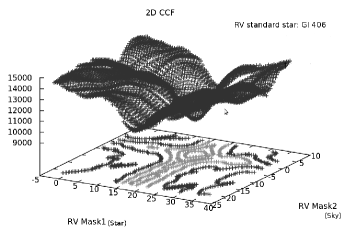
Figure 3: Resulting 2D CCF for the star Gl406 and telluric lines using an M6 stellar mask and an atmospheric mask, respectively. The best correlation is found for the atmosphere (RV Mask2) and the star (RV Mask1) at the lowest point of the function in the z-axis.

We note that during telluric removal the final S/N of the cleaned spectrum (C in Fig. 1) decreased to about $\sim$20. The S/N of individual nodded positions was often low. Therefore, with the exceptions of the sources GSS26 and GY23 and the RV standards, we combined the nodded spectra to form a single spectrum in order to increase the final S/N.

In addition, we also included an algorithm (analog to the continuum task from the IRAF package) to better fit the noisy continuum around each spectral line used in the cross-correlation. This last procedure had the effect of ”cleaning” the final shape of the CCF from spurious spatial frequencies introduced by the incorrect fitting of the continuum level in the noisiest spectra.

2.3 Results

The RV measurements of stars that possess multi-epoch observations are shown in Table 1 and are plotted in Fig. 4 and 6. Final RVs come from the 2D CCFs calculated using the spectral information in the wavelength region of the CO $\Delta\nu$ = (0-2) bandhead window sampled in DET4 in the chosen CRIRES setting ($\sim$ 14 absorption lines). The errors quoted in Table 1 were computed as follows. For each independent exposure (nodded spectrum), an RV was derived for each of the 14 lines in the region of the CO $\Delta\nu$ = (0-2) bandhead. A weighted mean was calculated using the line depth as weight. An average deviation of the 14 RVs was then computed. The final $\sigma$ quoted in Table 1 is then the average $\sigma$ divided by $N^{1/2}$, where $N$ is the number of the total nodded spectra. Errors for GSS26, GY23 and the RV standards (HD129642, HD105671, Gl406) were computed as described above. For the remaining targets where we had to combine all available exposures, the errors presented in Table 1 are the RMS of the RVs computed using the 14 lines. The errors range from around 0.015 (in GSS26) to 1.20 kms^-1 in the noisier stars (S/N$\sim$15).
We caution that the low errors obtained for some stars in Table 1 are probably underestimated. According to Figueira et al. (2010a) and Figueira et al. (2010b), the precision one can obtain using the telluric lines as zero-point is better than 10m s^-1. This is about what we obtain on the RV standards. On the one hand these low uncertainties are telling us that the systematic errors (target centering, detector characteristics, etc.) are not dramatically higher than those fund on the time-scale of our measurements (100 days or so). On the other, they might simply reflect the low-number of measurements obtained for our targets. A more realistic estimation of the errors will therefore be obtained later in our survey.

To assess the precision obtained by the method presented here, we computed the RV for the RV standards Gl406, HD129642, and HD105671. For Gl406, we obtain 19.730 kms^-1 with an internal dispersion of 0.010 kms^-1 in all nodded images. Our results is very close to the published result provided in White & Basri (2003) of 19.175 kms^-1 and to the 19.18$\pm$0.03 km s^-1 obtained over 11 measurements (Forveille, private communication). Quite striking is the RV = -4.59 kms^-1 and the low dispersion ($\sim$0.08 kms^-1) obtained in the four different epochs in the star HD129642. Results are plotted in Fig 4. An RV precise value of -4.60 kms^-1 is given by Gontcharov (2006). The four epochs obtained for HD129642 coincide with the temporal window of most of our Class I/II sources. That they are able to reproduce HD129642 RV during such an extended period confirms the stability and precision of the results.

Figure 4: RV measurements for the STD star HD129642. Error bars come from the relation <$\sigma_{vrad}$>* N^-1/2 being $\sigma_{vrad}$ the dispersion of the RV determined in each nodded image and N the number of individual measurements.

3 Discussion

3.1 Origin of the CO: photospheric or circumstellar

Protostellar light is often reprocessed in the circumstellar environment and becomes contaminated with emission or absorption from different origins. Particularly in the near-IR the circumstellar disk is thought to play a central role (Calvet et al., 1991) in altering the stellar signature because the temperatures of the excited material emit in the same wavelength as the protostellar photosphere.
For the CO regions, for instance, dedicated studies in TTS with accretion disks (e.g. Carr et al., 1993; Najita et al., 1996; Luhman & Rieke, 1999) have uncovered observations of CO overtone bandheads. The presence of inclined circumstellar disks can affect the shape of observed CO spectral lines that can exhibit anomalous double peaking profiles or depict a wider velocity field gradient. These features can be observed mainly in emission, but can also be found in absorption (see e.g. Hoffmeister et al., 2006, and references therein) and are apparently associated with the most active PMS sources such as the Fu Orionis objects (Hartmann et al., 2004). CO absorption lines can be produced in a circumstellar disk when its temperature profile depicts a negative vertical gradient very much like a stellar photosphere (see e.g. Käufl et al., 2005).
Nevertheless, because the dynamics of the material in circumstellar disks present Keplerian velocity profiles (Casali & Eiroa, 1996), the CO absorption of circumstellar nature drastically contrasts with the CO absorption profiles of photospheric origin. High-resolution observations are usually able to separate both components.

Figure 5: Observed protostellar spectra that we were able to reproduce with rotationally broadened stellar photospheric profiles. Right panel: Overplotted are some synthetic spectra (with a fixed T_eff of 3649K) (solid lines) with different vsini rotations with the spectrum of the protostar GY23 on one of the dates it was observed. Left panel: The same, but with a fixed vsini of 17kms^-1 and different temperatures.

In Fig. 5 we show that our protostellar spectra can be reproduced by rotationally broadened photospheric synthetic spectra. As an example in this figure, we rotationally broadened 5 solar metallicity PHOENIX stellar models of Spectral type G8V, K2V, K5V, M1 and M6 (T_eff ranging from 5650K to 3050K) with the same resolution as our observations and overplotted them with the spectrum of the source GY23. The match between the synthetic and the observed profiles is evident. Using different sets of models we were able to extend this result to all 7 protostars presented in this work. For this reason we believe that the lines analyzed here are generated in a photospheric environment and that the RVs found are of stellar origin.

3.2 Radial velocities

Table 1: Barycentric Julian dates of each target, derived RVs, and final dispersion for each date it was observed. In the upper table the results from each nodded image are presented. In the lower panel we show the RV measurements in images of sources that yielded an insufficiently S/N after telluric removal and that had to be combined for better precision.

Source	MJD	vrad [km s-1]	<$\sigma$>	Source	MJD	vrad [km s-1]	<$\sigma$>
nodded images
GSS 26	2454584.63565	-6.97198		HD129642	2454584.62788	-4.48490
	2454584.63909	-6.93852			2454584.63176	-4.59242
	2454584.63745	-6.94756			2454584.62387	-4.22596
	2454584.64087	-6.96722	0.01		2454584.61976	-4.59242
	2454595.81134	-6.93863			2454584.63573	-4.60915
	2454595.81313	-7.03562			2454584.63931	-4.26827	0.09
	2454595.81492	-6.95636			2454595.76527	-4.48264
	2454595.81664	-6.89839	0.03		2454595.76193	-4.71534
	2454700.50155	-6.98628			2454595.75729	-4.67921
	2454700.50334	-6.99655			2454595.75303	-4.64180
	2454700.50501	-6.94632			2454595.76937	-4.72930
	2454700.50681	-6.86636	0.03		2454595.77303	-4.82873	0.06
GY23	2454584.66269	-11.74129			2454696.51517	-4.59595
	2454584.66334	-11.91061			2454696.51934	-4.49518
	2454584.66383	-11.61631			2454696.51108	-4.63937
	2454584.66435	-11.92826	0.07		2454696.50713	-4.34328
	2454595.80848	-6.86636			2454696.52319	-4.60013
	2454595.80786	-6.99655			2454696.52733	-4.75527	0.07
	2454595.80737	-6.94632			2454712.50231	-4.80776
	2454595.80672	-6.82011	0.04		2454712.50480	-4.59263
	2454710.51703	-10.14933			2454712.50349	-4.68273
	2454710.51638	-9.97590			2454712.50343	-4.72138
	2454710.51590	-10.23329			2454712.50391	-4.44132
	2454710.51526	-10.11078	0.05		2454712.50429	-4.62820	0.07
Gl 406	2454890.64318	19.73374		HD105671	2454795.13436	-4.20193
	2454890.64215	19.72979			2454795.13447	-4.22028	0.01
	2454890.64125	19.74171
	2454890.64024	19.70016	0.01
combined images
GY 51	2454584.67379	-10.75198	0.22	L 1689 SNO2	2454699.66023	-7.76361	0.76
	2454595.83890	-9.44251	0.35		2454873.87196	-7.26417	0.56
	2454597.72588	-6.26190	0.25		2454884.87905	-5.76223	0.92
	2454710.527356	-10.18371	0.73
VSSG 18	2454597.88737	-15.89123	0.28	IRS 34	2454597.80272	-7.36514	0.63
	2454612.72451	-13.73072	0.32		2454612.80033	-7.17129	0.80
	2454733.55090	-17.12639	0.44		2454712.56017	-7.25198	1.22
WL 17	2454597.75984	-5.62187	0.65
	2454610.76480	-6.12428	1.10

From the RV measurements presented in Table 1 we can see that the range of values obtained (from $\sim$ -5.5 to -17 kms^-1) seems to indicate that the sources studied here are indeed from the $\rho$ Ophiuchus cloud. All targets, with the exception of VSSG18, are within 3 $\sigma$ of the characteristic velocities exhibited by $\rho$Oph sources, -6.3 $\pm$ 1.0 kms^-1 (Kurosawa et al., 2006; Prato, 2007).
The phenomenon of accretion and stellar activity in protostellar ages has the effect of altering spectral line-shapes. These non-periodical variations change the line-shape and induce RV variations that can reach amplitudes of the order on the $\sim$2-3 kms^-1 (e.g. Alencar et al., 2005). Therefore, although it is possible that some of the observed RV variations might be caused by stellar activity and accretion, the amplitude of the variations ($\simeq$ 4-6 kms^-1) observed for VSSG18, GY23, and GY51 suggests that those variations could have been caused by a spectroscopic companion.

Figure 6: Radial velocity measurements of the 7 protostars of our sample. Error bars in GSS26 and GY23 are calculated from the relation <$\sigma_{vrad}$>* N^-1/2 being $\sigma_{vrad}$ the dispersion of the RV determined in each nodded image and N the number of individual measurements. In all others targets error bars were computed as explained in Sect. 2.4..

Moreover, for the other 3 proto-stars observed with lower S/R (IRS34, L1689SNO2 and WL17) low-amplitude RV variations were detected, suggesting that the RV variations found among VSSG18, GY23, and GY51 might well be produced by companions. Because the effects of this accretion-driven RV modulation do not persist for long (see ibid), the only way to confirm the nature of the observed variations is to assess the eventual variations of the orbital parameters. In particular, variations of the semi-amplitude and/or the phase would indicate that the RV modulations are likely to be accretion-driven (e.g. Huélamo et al., 2008).

Finally, concerning VSSG18 alone, all RV measurements are well above the 3 $\sigma$ of the mean of the velocity distribution of $\rho$Oph from Kurosawa et al. (2006). VSSG18 average velocity is of -15.873 kms^-1, a clear but not extreme outlier from the local cloud. Based on its spectral energy distribution and spectral index from previous imaging studies it seems that VSSG18 is indeed a proto-star. Its deviant RV could suggest that this is long-period SB1 system.

3.3 Multiplicity and star formation scenarios

The use of CRIRES along with the technique described in the present work allowed us for the first time to carry out a systematic search for spectroscopic companions at early stages of their formation (below about 1Myr or so). Although preliminary and covering a small number of objects (7 objects only), the present paper brings already some interesting aspects concerning the configuration where those systems are found.

Out of 7 sources, 4 are known to be in multiple visual systems, namely, L1689NO2 (Haisch et al., 2004), IRS34 (Barsony et al., 2005), GY51 (Haisch et al., 2006), and GY23 (Elias, 1978; Haisch et al., 2002, 2004), whereas the other 3 targets (GSS26, WL17 and VSSG18) did not have any detected companions in previous imaging surveys (Haisch et al., 2004, 2006; Barsony et al., 2005; Duchêne et al., 2004).

GY51 and GY23 resemble some young multiple systems found in the literature. The former, is maybe a non-hierarchical system such as HD 34700 (Sterzik et al., 2005) whereas the latter looks like to be in the typical hierarchical configuration with a tight inner binary with an additional companion which probably caused the inner orbital evolution of the inner pair (Tokovinin et al., 2006).

The detection of a potential spectroscopic VSSG18 system without visual companion detected is interesting. If we believe that one possible (or maybe the only possible) way to form spectroscopic pairs is through the existence of an additional companion, systems such as VSSG18 are valuable because, if confirmed, they might set time constraints for orbital evolution to occur. Also, they could be interesting targets for AO-assisted campaigns to look for more close companions.

When we combinethe results of our study with those of Haisch et al. (2004, 2006), Barsony et al. (2005), and Duchêne et al. (2004), there were 2 single systems (S) amongst the YSO analyzed systems, 3 binaries (B), 1 triple (T) (1 spectroscopic binary + 1visual companion), and one quadruple (Q) (1 spectroscopic binary + 3 visual companions). The binary fraction (BF) of this small sample of protostars ($B+T+Q)/\leavevmode\nobreak\ (S+B+T+Q$) is $\simeq$71%. This preliminary result, although based on such a small sample, agrees surprisingly well with the notion that multiplicity is very high at young ages and therefore it might be a product of star formation. We advise caution in the interpretation of this final BF, however, because it is likely affected by low number statistics and it requires confirmation with a larger sample of protostars.

4 Conclusions

We have performed a spectroscopic multi-epoch survey of 7 known protostars in the $\rho$Ophiuchus star-forming region in the near-IR. Our main goal was to derive the close-binary frequency of embedded sources where multiplicity is already known from imaging techniques. We successfully derived radial velocities of Class I/II sources with an unprecedented precision in the spectroscopic study of protostars. Depending on the orbital period, our method allows for the detection of companions within the planetary-mass domain around embedded sources.
We find tentative evidence for the existence of three spectroscopic multiple systems out of the total 7 protostars analyzed. With an internal precision in the range of 0.02 to 1.22 kms^-1 we detected clear RV variations on the order of 4 to 6 kms^-1. When we combined our results with those of other studies, we obtain a binary fraction of $\simeq$71.5% for these systems, which is in line with the idea that multiplicity is high at protostellar ages. The existence of such young SBs strengthens the notion that dynamical evolution has already taken place in the Class I/ II phase (ages $\sim 10^{5}$ yrs).
Future observations are needed to enhance the sample statistics and will aim to derive the orbital solutions for these SBs if their multiple system status is confirmed.

Table 2: From left to right we present the star-forming region of each target, the coordinates, observation date, integration time of our observations, K-magnitude, the number of nodding cycles observed, the S/N*, the signal to noise ratio of the extracted spectra before telluric removal, the spectral energy distribution (SED), the reference from where the SEDs were collected and an alternative name for each source, if available.

Source	Region	$\alpha(2000)$	$\delta(2000)$	Date	DIT(sec)	K (mag)	nod.cy	S/N*	SED	reference	alias
Ced 110 IRS6	Cha	11 07 09.80	-77 23 04.4	2008-04-28	180.0	10.9	2	25	FS	Hai06	PCW91
				2008-12-27	180.0		2	30
				2008-12-28	180.0		2	30
				2009-02-23	180.0		2	25
Cha I T29	Cha	11 07 59.25	-77 38 43.9	2008-04-28	30.0	7.2	2	25	Class 0	Hai04 , Hai06	V* FK Cha
				2008-12-27	30.0		2	30
				2008-12-28	30.0		2	20
				2009-02-23	30.0		2	20
ISO-Cha I 26	Cha	11 08 04.00	-77 38 42.0	2008-04-28	45.0	8.2	2	30	Class I	Hai04 , Hai06	HD 97048 2
				2008-12-28	45.0		2	25
				2009-02-23	45.0		2	30
Cha I T32	Cha	11 08 04.61	-77 39 16.9	2008-04-28	30.0	6.1	2	25	Class 0	Hai04 , Hai06
				2008-12-28	30.0		2	25
				2009-02-23	30.0		2	25
Cha I T33B	Cha	11 08 15.69	-77 33 47.1	2008-04-28	30.0	6.9	2	30	FS	Hai06	Glass Ia
				2008-12-28	30.0		2	35
				2009-02-23	30.0		2	30
Cha I C9-2	Cha	11 08 37.37	-77 43 53.5	2008-04-28	45.0	8.6	2	20	Class 0	Hai04 , Hai06
				2008-12-28	45.0		2	20
				2009-02-10	45.0		2	25
				2009-02-26	45.0		2	20
Cha I C1-6	Cha	11 09 23.30	-76 34 36.2	2008-04-28	45.0	8.4	2	25	Class I	Hai04 , Hai06	CCE98 1-76
				2008-12-28	45.0		2	30
				2009-02-26	45.0		2	25
Cha I T41	Cha	11 09 50.39	-76 36 47.6	2008-04-28	30.0	7.0	2	30	-	-
				2008-12-28	30.0		2	25
				2009-02-26	30.0		2	25
Cha I T42	Cha	11 09 54.66	-76 34 23.7	2008-04-28	30.0	7.0	2	20	Class 0	Hai04 , Hai06	V* FM Cha
				2009-02-10	30.0		2	20
				2009-02-26	30.0		2	20
Cha I T44	Cha	11 10 01.35	-76 34 55.8	2008-04-28	30.0	6.4	2	20	Class 0	Hai04 , Hai06	CHXR 44
				2009-02-10	30.0		2	30
				2009-02-26	30.0		2	25
Cha I T47	Cha	11 10 50.78	-77 17 50.6	2008-04-28	45.0	8.8	2	20	-	-	V* FO Cha
				2009-02-11	45.0		2	30
				2009-02-26	45.0		2	20
Cha II 8	Cha	12 53 42.88	-77 15 05.7	2008-05-11	45.0	8.8	2	25	-	-
				2008-08-17	45.0		2	20
				2008-08-21	45.0		2	30
GSS 26	$\rho$Oph	16 26 10.28	-24 20 56.6	2008-04-28	120.0	9.4	2	25	Class I	Bar05
				2008-05-09	120.0		2	35
				2008-08-21	120.0		2	30
GSS/IRS 1	$\rho$Oph	16 26 21.50	-24 23 07.0	2008-04-28	120.0	9.0	2	30	Class I	Bar05
				2008-05-09	120.0		2	20
				2008-09-01	120.0		2	30
GY 23	$\rho$Oph	16 26 24.00	-24 24 49.9	2008-04-28	30.0	7.4	2	30	Class II	Bar05	S2
				2008-05-09	30.0		2	25
				2008-09-01	30.0		2	30
GY 51	$\rho$Oph	16 26 30.49	-24 22 59.0	2008-04-28	180.0	10.2	2	30	FS	Hai06	VSSG27
				2008-05-09	180.0		2	30
				2008-05-11	180.0		2	35
				2008-09-01	180.0		2	25
WL 12	$\rho$Oph	16 26 44.30	-24 34 47.5	2008-04-28	180.0	10.4	2	15	Class I	Bar05	GY111
				2008-05-09	180.0		2	20
				2008-09-02	180.0		2	20
WL 1 S	$\rho$Oph	16 27 04.13	-24 28 30.7	2008-05-09	180.0	10.8	2	25	Class II	Bar05
				2008-05-13	180.0		2	20
WL 17	$\rho$Oph	16 27 06.79	-24 38 14.6	2008-05-11	180.0	10.3	2	25	Class I	Bar05	GY205
				2008-05-24	180.0		2	20
Elias 29	$\rho$Oph	16 27 09.43	-24 37 18.5	2008-05-11	30.0	7.5	2	25	Class 0	Hai04 , Hai06	GY214
				2008-05-26	30.0		2	20
				2008-09-03	30.0		2	20
GY 224	$\rho$Oph	16 27 11.17	-24 40 46.7	2008-05-11	180.0	10.8	2	20	FS	Bar05	WLY 1-43
				2008-05-24	180.0		2	30
				2008-09-03	180.0		2	25
IRS 34	$\rho$Oph	16 27 15.48	-24 26 40.6	2008-05-11	180.0	10.3	2	25	FS	Bar05	GY239
				2008-05-26	180.0		2	25
				2008-09-03	180.0		2	30
IRS 37	$\rho$Oph	16 27 17.54	-24 28 56.5	2008-05-11	180.0	10.9	2	25	Class I	Hai04	GY244
				2008-05-26	180.0		2	25
				2008-09-24	180.0		2	25
IRS 42	$\rho$Oph	16 27 21.45	-24 41 42.8	2008-05-11	45.0	8.6	2	25	FS	Bar05	GY252
				2008-05-24	45.0		2	30
				2008-09-24	45.0		2	30
WL 6	$\rho$Oph	16 27 21.83	-24 29 53.2	2008-05-11	180.0	10.8	2	35	Class I	Bar05	GY254
				2008-09-24	180.0		2	30
				2008-09-25	180.0		2	30
IRS 43	$\rho$Oph	16 27 26.90	-24 40 51.5	2008-05-11	120.0	9.4	2	25	Class I	Bar05	GY265
				2008-05-24	120.0		2	20
				2008-09-03	120.0		2	25
IRS 44	$\rho$Oph	16 27 28.00	-24 39 34.3	2008-05-11	120.0	9.7	2	30	Class I	Bar05	GY269
				2008-05-24	120.0		2	20
				2008-09-03	120.0		2	30
VSSG 18	$\rho$Oph	16 27 28.44	-24 27 21.9	2008-05-11	120.0	9.2	2	30	FS	Bar05
				2008-05-26	120.0		2	30
				2008-09-24	120.0		2	30
IRS 46	$\rho$Oph	16 27 29.70	-24 39 16.0	2008-05-11	180.0	10.6	2	20	Class I	Bar05	GY274
				2008-05-26	180.0		2	20
				2009-02-23	180.0		2	30
GY 279	$\rho$Oph	16 27 30.18	-24 27 44.3	2008-05-11	45.0	9.0	2	30	FS	Bar05	IRS47
				2008-05-26	45.0		2	20
				2008-09-25	45.0		2	25
IRS 48	$\rho$Oph	16 27 37.20	-24 30 34.0	2008-05-11	30.0	7.7	2	20	FS	Hai06	GY304
				2008-05-26	30.0		2	25
				2009-02-22	30.0		2	25
IRS 51 S	$\rho$Oph	16 27 39.84	-24 43 16.1	2008-08-21	45.0	8.7	2	20	FS	Hai06	GY315
				2008-09-03	45.0		2	25
				2009-02-22	45.0		2	30
IRS 54	$\rho$Oph	16 27 51.70	-24 31 46.0	2008-08-21	180.0	10.2	2	20	Class I	Hai06	GY378
				2009-02-12	180.0		2	25
				2009-02-22	180.0		2	30
IRS 63	$\rho$Oph	16 31 35.53	-24 01 28.3	2008-08-21	120.0	9.3	2	25	Class I	Hai02 , Hai06	WLY 2-63
				2009-02-11	30.0		2	30
				2009-02-23	30.0		2	20
L1689SNO2N	$\rho$Oph	16 31 52.13	-24 56 15.2	2008-08-21	45.0	8.3	2	30	FS	Hai06
				2009-02-11	45.0		2	20
				2009-02-22	45.0		2	25
IRS 67	$\rho$Oph	16 32 01.00	-24 56 44.0	2008-08-25	180.0	10.3	2	20	Class I	Hai02 , Hai06
				2009-02-11	180.0		2	30
				2009-02-23	180.0		2	20
SVS 20 S	Serpens	18 29 57.70	+01 14 07.0	2008-05-09	30.0	7.1	2	20	FS	Hai06
				2008-05-22	30.0		2	20
				2008-05-26	30.0		2	25
				2008-08-21	30.0		2	30
EC 95	Serpens	18 29 57.80	+01 12 52.0	2008-05-09	120.0	9.8	2	25	Class II	Hai06
				2008-05-22	120.0		2	20
				2008-05-26	120.0		2	30
				2008-08-21	120.0		2	20
Radial velocity standards
HD 129642		14 45 09.74	-49 54 58.61	2008-04-28	120.0	6.2	3	110
				2008-05-09	120.0		3	120
				18 aug 2008	120.0		3	130
				2008-09-03	120.0		3	120
HD 105671		12 09 54.98	-46 12 30.20	2008-12-28	60.0	5.8	2	150
Gl 406		10 56 28.86	+07 00 52.77	28 feb 2009	60.0	6.1	2	120

Table 2: Cont.