Block local elimination algorithms for solving sparse discrete optimization problems

Abstract

Block elimination algorithms for solving sparse discrete optimization problems are considered. The numerical example is provided. The benchmarking is done in order to define real computational capabilities of block elimination algorithms combined with SYMPHONY solver. Analysis of the results show that for sufficiently large number of blocks and small enough size of separators between the blocks for staircase integer linear programming problem the local elimination algorithms in combination with a solver for solving subproblems in blocks allow to solve such problems much faster than used solver itself for solving the whole problem. Also the capabilities of postoptimal analysis (warm starting) are considered for solving packages of integer linear programming problems for corresponding blocks.

1 Introduction

The use of discrete optimization (DO) models and algorithms makes it possible to solve many practical problems, since the discrete optimization models correctly represent the nonlinear dependence, indivisibility of an objects, consider the limitations of logical type and all sorts of technology requirements, including those that have qualitative character. But unfortunately, most of the interesting problems are in the complexity class $NP$-hard and may require searching a tree of exponential size in the worst case. Many real DOPs from OR applications contain a huge number of variables and/or constraints that make the models intractable for currently available solvers. Usually, DOPs from applications have a special structure, and the matrices of constraints for large-scale problems have a lot of zero elements (sparse matrices), and the nonzero elements of the matrix often fall into a limited number of blocks. The block form of many DO problems is usually caused by the weak connectedness of subsystems of real-world systems.

Among the block structures let us pay particular attention to the block-tree structure, a special case of which is a staircase or quasiblock structure (Fig. 1). The problems of optimal reservation of hotel rooms Soa83 have the quasiblock structure, similar to the previous temporal knapsack problems Bartlett , recently received the application in solving problems of the prior reservation of computing resources in the Grid Computing.

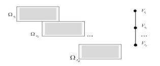
Figure 1: Quasi-block structure.

One of the promising ways to exploit sparsity in the constraint matrix of DO problems are local elimination algorithms (LEA)Shc2 , including local decomposition algorithms Soa83 , nonserial dynamic programming (NSDP) Bertele algorithms, Soa07 . To extract special block structures there are such promising graph-based decomposition approaches as methods of tree decomposition SoaKibern07 . The purpose of this paper to define real computational capabilities of block elimination algorithms combined with modern solvers.

2 Local elimination algorithms for solving discrete problems

2.1 General scheme of local elimination algorithms

In the papers Shc2 , Soa09 considered the general class of local elimination algorithms for computing information, that have decomposition approach and that allow to calculate some global information about a solution of the entire problem using local computations.

A local elimination algorithm (LEA) eliminates local elements of the problem’s structure defined by the structural graph by computing and storing local information about these elements in the form of new dependencies added to the problem.

The local elimination procedure consists of two parts:

• The forward part eliminates elements, computes and stores local solutions, and finally computes the value of the objective function;

• The backward part finds the global solution of the whole problem using the tables of local solutions; the global solution gives the optimal value of the objective function found while performing the forward part of the procedure.

The algorithmic scheme of the LEA is a directed acyclic graph (DAG) in which the vertices correspond to the local subproblems and the edges reflect the informational dependence of the subproblems on each other.

It is important that aforementioned methods use just the local information (i.e., information about elements of given element’s neighborhood) in a process of solving discrete problems. Thus local elimination algorithms allow to calculate some global information about a solution of the entire problem using local computations.

The structure of discrete optimization problems is determined either by the original elements (e.g., variables) with a system of neighborhoods specified for them with help of structural graph and with the order of searching through those elements using a LEA or by various derived structures (e.g., block or tree-block structures).

2.2 Local elimination algorithms

Consider LEA in details for solving sparse problems of integer linear programming in the case when structural graph is interaction graph of variables, which is also called constraint graph.

Consider the integer linear programming (ILP) problem with binary variables

$$f(X)=CX=\sum_{j=1}^{n}c_{j}x_{j}\rightarrow\max$$ (1)

subject to constraints

$$\sum_{j=1}^{n}a_{ij}x_{j}\leq b_{i},i=1,2,\dots,m,$$ (2)

$$x_{j}=0,1,j=1,2,\dots,n.$$ (3)

Definition 1

Variables $x$ and $y$ interact in ILP problem with constraints if they both appear in the same constraint.

Definition 2

Interaction graph of the ILP problem is an undirected graph $G=(X,E)$, such that

• Vertices $X$ of $G$ correspond to variables of the ILP problem;

• Two vertices of $G$ are adjacent iff corresponding variables interact.

Further, we shall use the notion of vertices that correspond one-to-one to variables.

Example 1

Consider an ILP problem with binary variables:

$$2x_{1}+3x_{2}+~{}x_{3}+5x_{4}+4x_{5}+6x_{6}+~{}x_{7} \rightarrow\max$$ (4)

subject to constraints

$$3x_{1}+4x_{2}+~{}~{}x_{3}~{}~{}~{}~{}~{}~{}~{}~{}~{}~{}~{}~{}~{}~{}~{}~{}~{}~{}~{}~{}~{}~{}~{}~{}~{}~{} ~{}~{}~{}~{}~{}\leq 6,$$ (5)

$$~{}~{}~{}~{}~{}~{}~{}~{}2x_{2}+3x_{3}+3x_{4}~{}~{}~{}~{}~{}~{}~{}~{}~{}~{}~{}~{}~{}~{}~{}~{}~{}~{} ~{}~{}~{}~{}~{}\leq 5,$$ (6)

$$~{}~{}~{}~{}~{}~{}~{}~{}2x_{2}~{}~{}~{}~{}~{}~{}~{}~{}~{}~{}~{}~{}~{}~{}~{}~{}+3x_{5}~{}~{}~{}~{}~{}~{}~{} ~{}~{}~{}~{}~{}~{}~{}~{}\leq 4,$$ (7)

$$~{}~{}~{}~{}~{}~{}~{}~{}~{}~{}~{}~{}~{}~{}~{}~{}2x_{3}~{}~{}~{}~{}~{}~{}~{}~{}~{}~{}~{}~{}~{}~{}~{}~{}+3x_{6}+2x_{7} \leq 5,$$ (8)

$$~{}x_{j}=0,1,~{}j=1,\ldots,7.~{}~{}~{}~{}~{}~{}~{}~{}~{}~{}~{}~{}~{}~{}~{}~{}~{}~{}~{}~{}~{}~{}~{}~{}~{}~{}~{}~{}~{}~{}~{}~{}~{}$$ (9)

Definition 3

Two vertices $x$ and $y$ of $G=(X,E)$ are called neighbors if $(x,y)\in E$.

Definition 4

Set of variables interacting with a variable $x\in X$ is denoted by $Nb(x)$ and called the neighborhood of the variable $x$. For corresponding vertices a neighborhood of a vertex $x$ is a set of vertices of interaction graph $G=(X,E)$ that are linked by edges with $x$. Denote the latter neighborhood as $Nb_{G}(x)$.

The solution of a sparse discrete optimization problem (1) – (3) whose structure is described by an undirected interaction graph $G=(X,E)$ with help of LEA was described in SavSoa in details. Given an ordering $x_{1},x_{2},\dots,x_{n}$, the LEA proceeds in the following way: it subsequently eliminates $x_{1},x_{2},\dots,x_{n}$ in the current graph and computes an associated local information about vertices from $h_{i}(Nb(x_{i}))$. This process creates a sequence of elimination graphs: $G^{0}=G,G^{1},\dots,G^{j},\dots,G^{n}$, where $G^{n}=\emptyset$.

The process of interaction graph transformation corresponding to the LEA scheme is known as elimination game which was first introduced by Parter as a graph analogy of Gaussian elimination.

2.3 Block local elimination algorithms

The local elimination procedure can be applied to elimination of not only separate variables but also to sets of variables and can use the so called elimination of variables in blocks, which allows to eliminate several variables in block.

Applying the method of merging variables into meta-variables allows to obtain condensed or meta-DOPs which have a simpler structure. If the resulting meta-DOP has a nice structure (e.g., a tree structure) then it can be solved efficiently.

An ordered partition of a set $X$ is a decomposition of $X$ into ordered sequence of pairwise disjoint nonempty subsets whose union is all of $X$.

In general, graph partitioning is $NP$-hard. Since graph partitioning is difficult in general, there is a need for approximation algorithms. A popular algorithm in this respect is MeTiS, which has a good implementation available in the public domain.

An important special case of partitions are so-called blocks. Two variables are indistinguishable if they have the same closed neighborhood. A block is a maximal set of indistinguishable vertices. The blocks of $G$ partition $X$ since indistinguishability is an equivalence relation defined on the original vertices. The corresponding graph is called condensed graph, which is a merged form of original graph. Not formally, a condensed graph is formed by merging all vertices with the same neighborhoods into a single meta-node (supervariable).

An equivalence relation on a set induces a partition on it, and also any partition induces an equivalence relation. Given a graph $G=(X,E)$, let $X$ be a partition on the vertex set $X$: $X={x_{1},x_{2},\dots,x_{p}}$, $p\leq n$, where $x_{l}=X_{K_{l}}$($K_{l}$ is a set of indices corresponding to $x_{l}$, $l=1,\dots,p$). For this ordered partition $X$, the DOP (1) – (3) can be solved by the LEA using quotient interaction graph $G$.

That is, $\cup_{i=1}^{p}\mathbf{x_{i}}=X$ and $\mathbf{x_{i}}\cap\mathbf{x_{k}}=\emptyset$ for $i\neq k$. We define the quotient graph of $G$ with respect to the partition $\mathbf{X}$ to be the graph

$$\mathbf{G}=G/\mathbf{X}=(\mathbf{X},\mathcal{E}),$$

where $(\mathbf{x_{i}},~{}\mathbf{x_{k}})\in\mathcal{E}$ if and only if $Nb_{G}(\mathbf{x_{i}})\cap\mathbf{x_{k}}\neq\emptyset$.

The quotient graph $\mathbf{G}(\mathbf{X},\mathcal{E})$ is an equivalent representation of the interaction graph $G(X,E)$, where $\mathbf{X}$ is a set of blocks (or indistinguishable sets of vertices), and $\mathcal{E}\subseteq\mathbf{X}\times\mathbf{X}$ be the edges defined on $\mathbf{X}$. A local block elimination scheme is one in which the vertices of each block are eliminated contiguously. As an application of a clustering technique we consider below a block local elimination procedure where the elimination of the block (i.e., a subset of variables) can be seen as the merging of its variables into a meta-variable.

A. Forward part

Consider first the block $\mathbf{x_{1}}$. Then

$$\max_{X}\{C_{N}X_{N}|A_{iS_{i}}X_{S_{i}}\leq b_{i},~{}i\in M,~{}x_{j}=0,1,~{}j\in N\}=$$

$$\max_{X_{K_{2}},\ldots,X_{K_{p}}}\{C_{N-K_{1}}X_{N-K_{1}}+h_{1}(Nb(X_{K_{1}})|A_{iS_{i}}X_{S_{i}}\leq b_{i},~{}i\in M-U_{1},$$

$$x_{j}=0,1,~{}j\in N-K_{1}\}$$

where $U_{1}=\{i:S_{i}\cap K_{1}\neq\emptyset\}$ and

$$h_{1}(Nb(X_{K_{1}}))=\max_{X_{K_{1}}}\{C_{K_{1}}X_{K_{1}}|A_{iS_{i}}X_{S_{i}}\leq b_{i},~{}i\in U_{1},~{}x_{j}=0,1,~{}x_{j}\in Nb[\mathbf{x_{1}}]\}.$$

The first step of the local block elimination procedure consists of solving, using complete enumeration of $X_{K_{1}}$, the following optimization problem

$$h_{1}(Nb(X_{K_{1}}))=\max_{X_{K_{1}}}\{C_{K_{1}}X_{K_{1}}|A_{iS_{i}}X_{S_{i}}\leq b_{i},~{}i\in U_{1},~{}x_{j}=0,1,~{}x_{j}\in Nb[\mathbf{x_{1}}]\},$$ (10)

and storing the optimal local solutions $X_{K_{1}}$ as a function of the neighborhood $ofX_{K_{1}}$, i.e., $X_{K_{1}}^{*}(Nb(X_{K_{1}}))$.

The maximization of $f(X)$ over all feasible assignments $Nb(X_{K_{1}})$, is called the elimination of the block (or meta-variable) $X_{K_{1}}$. The optimization problem left after the elimination of $X_{K_{1}}$ is:

$$\max_{X-X_{K_{1}}}\{C_{N-K_{1}}X_{N-K_{1}}+h_{1}(Nb(X_{K_{1}}))|A_{iS_{i}}X_{S_{i}}\leq b_{i},~{}i\in M-U_{1},x_{j}=0,1,~{}j\in N-K_{1}\}.$$

Note that it has the same form as the original problem, and the tabular function $h_{1}(Nb(X_{K_{1}}))$ may be considered as a new component of the modified objective function. Subsequently, the same procedure may be applied to the elimination of the blocks – meta-variables $\mathbf{x_{2}}=X_{K_{2}},\ldots,\mathbf{x_{p}}=X_{K_{p}}$, in turn. At each step $j$ the new component $h_{\mathbf{x_{j}}}$ and optimal local solutions $X^{*}_{K_{j}}$ are stored as functions of $Nb(X_{K_{j}}\mid X_{K_{1}},\ldots,X_{K_{j-1}})$, i.e., the set of variables interacting with at least one variable of $X_{K_{j}}$ in the current problem, obtained from the original problem by the elimination of $X_{K_{1}},\ldots,X_{K_{j-1}}$. Since the set $Nb(X_{K_{p}}\mid X_{K_{1}},\ldots,X_{K_{p-1}})$ is empty, the elimination of $X_{K_{p}}$ yields the optimal value of objective $f(X)$.

B. Backward part.

This part of the procedure consists of the consecutive choice of $X^{*}_{K_{p}}$, $X^{*}_{K_{p-1}},\ldots,X^{*}_{K_{1}}$, i.e., the optimal local solutions from the stored tables $X^{*}_{K_{1}}(Nb(X_{K_{1}})),X^{*}_{K_{2}}(Nb(X_{K_{2}}\mid X_{K_{1}})),\ldots,X^{*}_{K_{p}}\mid X_{K_{p-1}},\ldots,X_{K_{1}}$.

Underlying DAG of the local block elimination procedure contains nodes corresponding to computing of functions $h_{\mathbf{x_{i}}}(Nb_{G_{\mathbf{X}}^{(i-1)}}(\mathbf{x_{i}}))$ and is a generalized elimination tree.

Example 2

Consider a DO problem (4) – (9) from example 1 and an ordered partition of the variables of the set $X$ into blocks: $\mathbf{x_{1}}=\{x_{5}\},\mathbf{x_{2}}=\{x_{1},x_{2},x_{4}\},\mathbf{x_{3}}=\{x_{6},x_{7}\},\mathbf{x_{4}}=\{x_{3}\}$. For the ordered partition $\{x_{1},x_{2},x_{3},x_{4}\}$, this DO problem may be solved by the LEA. Initial interaction graph with partition presented by dashed lines is shown in Fig. 2 (a), quotient interaction graph is in Fig. 2 (b), and the DAG of the block local elimination computational procedure is shown in Fig. 3.

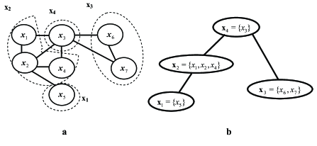
Figure 2: Interaction graph of the DOP with partition (dashed) (a) and quotient interaction graph (b) (example 2).

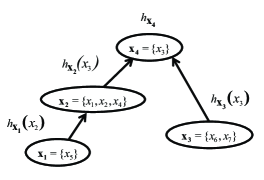
Figure 3: The DAG (generalized elimination tree) of the local block elimination computational procedure for the DO problem (example 2).

A. Forward part

Consider first the block $\mathbf{x_{1}}=\{x_{5}\}$. Then $Nb(\mathbf{x_{1}})=\{x_{2}\}$. Solve the following problem containing $x_{5}$ in the objective and the constraints:

$$h_{\mathbf{x_{1}}}(Nb(\mathbf{x_{1}}))=\max_{x_{5}}\{4x_{5}\mid 2x_{2}+3x_{5}\leq 4,x_{j}\in\{0,1\}\}$$

and store the optimal local solutions $\mathbf{x_{1}}$ as a function of a neighborhood, i.e., $\mathbf{x_{1}}^{*}(Nb(\mathbf{x_{1}}))$. Eliminate the block $\mathbf{x_{1}}$. and consider the block $\mathbf{x_{2}}=\{x_{1},x_{2},x_{4}\}$. $Nb(\mathbf{x_{2}})=\{x_{3}\}$. Now the problem to be solved is

$$h_{\mathbf{x_{2}}}(x_{3})=\max_{x_{1},x_{2},x_{4}}\{h_{\mathbf{x_{1}}}(x_{2})+2x_{1}+3x_{2}+5x_{4}\}$$

subject to

$$~{}~{}~{}3x_{1}+4x_{2}+~{}x_{3}~{}~{}~{}~{}~{}~{}~{}~{}~{}~{}\leq 6,$$

$$~{}~{}~{}~{}~{}~{}~{}~{}~{}~{}~{}~{}2x_{2}+3x_{3}+3x_{4}~{}\leq 5,$$

$$~{}~{}~{}~{}~{}~{}~{}~{}~{}~{}~{}~{}~{}~{}~{}~{}~{}~{}~{}~{}~{}~{}~{}x_{j}=0,1,~{}j=1,2,3,4.~{}~{}~{}~{}~{}~{}~{}~{}~{}~{}~{}~{}~{}~{}~{}~{}~{}~{}~{}~{}~{}~{}~{}~{}~{}~{}~{}~{}~{}~{}~{}~{}$$

Build the corresponding table 2.

Table 1.

Calculation of $h_{\mathbf{x_{1}}}(x_{2})$
$x_{2}$ $h_{\mathbf{x_{1}}}(x_{2})$ $x_{5}^{*}$ 0 4 1 1 0 0

Table 2.

Calculation of $h_{\mathbf{x_{2}}}(x_{3})$
$x_{3}$ $h_{\mathbf{x_{2}}}(x_{3})$ $x_{1}^{*}$ $x_{2}^{*}$ $x_{4}^{*}$ 0 11 1 0 1 1 6 1 0 0

Eliminate the block $\mathbf{x_{2}}$ and consider the block $\mathbf{x_{3}}=\{x_{6},x_{7}\}$. The neighbor of $\mathbf{x_{3}}$ is $x_{3}$: $Nb(\mathbf{x_{3}})=\{x_{3}\}$. Solve the DOP containing $x_{3}$:

$$h_{\mathbf{x_{3}}}(x_{3})=\max_{x_{6},x_{7}}\{h_{\mathbf{x_{2}}}+x_{3}+6x_{6}+x_{7}~{}|~{}2x_{3}+3x_{6}+2x_{7}\leq 5,x_{j}\in\{0,1\}\}$$

and build the table 3.

Table 3.

Calculation of $h_{\mathbf{x_{3}}}(x_{3})$
$x_{3}$ $h_{\mathbf{x_{3}}}(x_{3})$ $x_{6}^{*}$ $x_{7}^{*}$ 0 18 1 1 1 12 1 0

Eliminate the block $\mathbf{x_{3}}$ and consider the block $\mathbf{x_{4}}=\{x_{3}\}$. $Nb(\mathbf{x_{4}})=\emptyset$. Solve the DOP:

$$h_{\mathbf{x_{4}}}=\max_{x_{3}}\{h_{\mathbf{x_{3}}}(x_{3}),x_{j}\in\{0,1\}\}=18,$$

where $x_{3}^{*}=0$.

B. Backward part.

Consecutively find $\mathbf{x_{3}}^{*},\mathbf{x_{2}}^{*},\mathbf{x_{1}}^{*}$, i.e., the optimal local solutions from the stored tables 3, 2, 1. $x_{3}^{*}=0\Rightarrow x_{6}^{*}=1,~{}x_{7}^{*}=1$ (table 3); $x_{3}^{*}=0\Rightarrow x_{1}^{*}=1,~{}x_{2}^{*}=0,~{}x_{4}^{*}=1$ (table 2); $x_{2}^{*}=0\Rightarrow x_{5}^{*}=1$ (table 1). We found the optimal global solution to be $(1,~{}0,~{}0,~{}1,~{}1,~{}1,~{}1)$, the maximum objective value is 18.

3 Research the computational capability of local algorithms

3.1 Comparative computational experiment

Among extremely important research questions about the effectiveness of local elimination algorithms (LEA), the next one causes special interest: “Is the use of LEA in combination with a discrete optimization (DO) algorithm (for solving problems in the blocks) consistently more efficient than the standalone use of the DO algorithm?” Soa11 .

Along with the theoretical analysis of performance evaluations, it is of interest to provide a comparison of LEA combined with other DO algorithms by using computational experiments. Providing an exhaustive computational study for all possible combinations of LEA with all existing DO algorithms (or at least the most efficient ones) is extremely laborious. This work presents computational comparisons of the LEA combined with two DO algorithms: a) one of the least efficient DO algorithms, which is a simple implicit enumeration algorithm without use of linear relaxation; b) one of the most effective DO algorithm, as the one adopted by the simplex method in the unimodular case.

The purpose of these comparisons is to evaluate the behavior of the LEA in combination with very effective algorithms (“lower bound”) and weakly effective ones (“upper bound”).

By combining the LEA with implicit enumeration solvers (one of the least efficient algorithms) Soa83 we concluded that for sufficiently large number of blocks and small enough size of separators between the blocks for staircase ILP problems the performance is better than the stand alone solver. It has to be noted, that there are cases that the combination of LEA with the simplex method for a small number of blocks performs worse than the simplex method. Thus, the practical use of LEA in combination with a DO solver requires a preliminary machine experiment. Based on this experiment have to be determined the acceptable parameters for DO problems.

The paper ilSoa94 presents computational experiment on the effectiveness (in terms of precision and time to find a solution) of LEA in combination with approximate algorithms from the package of applied programs (PAP) “DISPRO” developed at the Institute of Cybernetics of Ukrainian Academy of Sciences. The studied methods include lexicographic search, recession vector and random search. The object of the experiments was a special class of DO quasi-block problems, the optimal reservation class, which under certain conditions are unimodular Soa83 . The results showed that if the efficiency of the PAP “DISPRO” algorithms is almost independent of the matrix condition structure of the DO problem, but is essentially determined by the dimension of the problem, then the use of LEA is appropriate for relatively small values of the separators and sufficient sparsity of the condition matrix.

Additionally, by using the LEA in combination with some DO algorithm we achieved better accuracy than by using just the DO algorithm. In some cases the time to solution is several times lower than the independent calculation with an appropriate DO algorithm. By increasing the dimension of the problem and by providing the resource time restriction the efficiency of the LEA increases.

3.2 SYMPHONY as a framework for solving mixed integer programming problems

The computational capabilities of the LEA in combination with a modern solver were tested by using SYMPHONY as the implementation framework. SYMPHONY is part of the COIN-OR project and it can solve mixed-integer linear programs (MILP) sequentially or in parallel. We chose this framework since it is open-source and supports warm restarts, which implement postoptimal analysis (PA) of ILP problems.

It has to be noted that SYMPHONY does not include an LP-Solver, but can use, through the Osi interface, third-party solvers such as Clp, Cplex, Xpress. Furthermore, SYMPHONY also has a structure-specific implementations for problems like the traveling salesman problem, vehicle routing problem, set partitioning problem, mixed postman problem and others.

Warm start technology for implementation of Postoptimal Analysis.

Warm restarts are used by modern solvers such as Gurobi, SCIP, CBC, SYMPHONY, and others, in order to implement PA. We use the capabilities of warm restarts offered by SYMPHONY in order to reduce the solution time of the subproblems generated by the computational scheme of LEA Soa08 .

SYMPHONY implements warm restarting by using a compact description of the search tree at the time the computation is halted. This description contains the complete information about the subproblem corresponding to each node in the search tree, including the branching decisions that leads to the creation of the node, the list of active variables and constraints, and warm restart information for the subproblem itself. All information is compactly stored using SYMPHONY’s native data structures, which store only the differences between a child and its parent, rather than an explicit description of every node. In addition to the tree itself, other relevant information regarding the status of the computation is recorded, such as the current bounds and best feasible solution.

By using warm restarting, the user can save a warm restart to disk, read one from the disk, or restart the computation at any point after modifying parameters or the problem data. Note that the use of the PA procedure does not always guarantee a positive result. In the case of SYMPHONY, it has been observed that, as a rule of thumb, the warm-restart procedure works best with a slight change in the conditions of the problem.

3.3 Benchmarking analysis

All experimental results were obtained on an Intel Core 2 Duo at 2.66 GHz machine with 2 GB main memory, and running Linux, version 2.6.35-24-generic. SYMPHONY 5.4.1 was used for the LEA implementation. The results are presented in Table 1, where $n$ denotes the number of variables, $m$ the number of constraints, $k$ the number of blocks, $b$ the size of separator, and underlined is the minimal time of problem solving for appropriate algorithm. The maximum solving time is denoted by $TIMEOUT$, and is equal to 2 hours.

Table 1: Run-time (in minutes) of solving generated problems with quasi-block structure.

	Problem parameters				Solvers
#	$n$	$m$	$k$	$b$	SYMPHONY	SYMPHONY + LEA	SYMPHONY + LEA + PA
1	180	12	6	1	9.503	0.028	0.026
2	180	12	6	2	3.019	0.046	0.047
3	180	12	6	3	1.671	0.17	0.171
4	180	12	6	4	1.164	0.493	0.485
5	180	12	6	5	0.084	5.667	5.295
6	180	50	25	5	1.572	0.03	0.031
7	180	12	6	6	2.7167	5.321	5.057
8	320	16	8	1	9.605	0.025	0.024
9	320	20	10	1	24.435	0.029	0.026
10	320	40	20	1	3.943	0.016	0.015
11	320	20	10	2	18.464	0.092	0.093
12	320	40	20	2	2.519	0.048	0.049
13	320	20	10	3	31	0.289	0.289
14	320	40	20	3	3.382	0.158	0.157
15	320	20	10	4	47.919	1.21	1.204
16	320	20	10	5	14.941	3.73	3.682
17	320	12	6	6	44.556	21.534	21.636
18	320	20	10	6	23.853	14.327	14.043
19	500	50	25	1	90.02	0.021	0.022
20	500	50	25	2	TIMEOUT	0.071	0.073
21	500	50	25	3	TIMEOUT	0.681	0.303
22	500	50	25	4	TIMEOUT	0.883	0.879
23	500	25	12	5	TIMEOUT	7.404	7.413
24	500	130	65	5	TIMEOUT	0.076	0.077
25	500	112	56	6	TIMEOUT	0.246	0.244
26	800	120	60	1	TIMEOUT	0.048	0.049
27	800	120	60	2	TIMEOUT	0.119	0.118
28	800	50	25	3	TIMEOUT	0.564	0.563
29	800	50	25	4	TIMEOUT	2.197	2.175
30	800	240	120	4	TIMEOUT	0.036	0.039
31	800	50	25	5	TIMEOUT	8.924	8.638
32	800	50	25	6	TIMEOUT	31.147	30.719
33	800	180	90	6	TIMEOUT	0.399	0.412
34	1000	50	25	1	TIMEOUT	0.073	0.075
35	1000	50	25	2	TIMEOUT	0.287	0.286
36	1000	50	25	3	TIMEOUT	1.07	1.071
37	1000	50	25	4	TIMEOUT	3.575	3.573
38	1000	50	25	5	TIMEOUT	14.424	16.327
39	1000	50	25	6	TIMEOUT	56.359	59.671
40	1000	250	125	6	TIMEOUT	0.569	0.577
41	1000	100	50	8	TIMEOUT	21.447	21.414

Test problem description. All the ILP problems with binary variables from a given experiment have artificially generated quasi-block structures. All the blocks from a single problem have the same number of variables, and also the same number of variables in separators between them. This is required in order to evaluate the impact of the PA on the time to solve the problem by increasing the number of variables.

The test problems were generated by specifying the number of variables, the number of constraints and the size of the separators between blocks. The number and the dimensions of the blocks were calculated by using the number of variables and constraints. The objective function and constraint matrix coefficients, and the right-hand sides for each of the block were generated by using a pseudorandom-number generator.

Each test problem was solved by using three algorithms, a) the basic MILP SYMPHONY solver with the $OsiSym$ interface, b) the LEA in combination with SYMPHONY, c) the LEA in combination with SYMPHONY and with PA (warm restarts). In all the cases SYMPHONY used preprocessing.

The computational experiments show that LEA combined with SYMPHONY for solving quasi-block problems with small separators outperforms the stand alone SYMPHONY solver (see table 1). Additionally, by increasing the size of the separators in the problems for the same number of variables and block sizes LEA becomes less efficient due to the increased number of iteration for solving the block subproblems. LEA’s efficiency is improved by using warm restarts. The ILP problems corresponding to the same block for different values of the separator variables differ only in the right-hand side. These problems can be solved partially by using warm restarts and information obtained from other problems, and this was expected to increase the LEA performance. However, the results show a inconsistent behavior. For most problems, the warm restarts don’t make a difference. For some problems, they improved the solution time (see problems 7, 17, 24), while for others they did not (see problems 5, 15, 40).

Concluding, there is not a definite answer for the block separator size that results to LEA’s lower performance (with respect to time to solution) compared to SYMPHONY. The performance depends on the problem structure; as the problem size increases LEA becomes more efficient.

4 Conclusion

The main result of this paper is to determine the real computational capabilities of block elimination algorithms combined with SYMPHONY solver. Analysis of the results show that for sufficiently large number of blocks and small enough size of separators between the blocks for staircase integer linear programming problem the local elimination algorithms in combination with a solver for solving subproblems in blocks allow to solve such problems much faster than used solver itself for solving the whole problem.

It seems promising to continue this line of research by studying capabilities of postoptimal analysis distributed by other modern solvers. It is also of interest to research computational capabilities of local algorithms for solving sparse problems of integer linear programming from real applications.

References

- (1) E. I. Ilovaiskaya and O. A. Shcherbina, On computational aspects of the realization of local algorithms for solution of problems of discrete optimization. Journal of Mathematical Sciences, 1994, 70, N 5, 2043–2046, DOI: 10.1007/BF02110838
- (2) O.A. Shcherbina. On local algorithms of solving discrete optimization problems, Problems of Cybernetics, Moscow, 1983, N 40, 171–200 (in Russian).
- (3) O. Shcherbina. Local Elimination Algorithms for Sparse Discrete Optimization Problems, D.Sc. Thesis, Moscow, Computer Centre of RAS, 2011, 357 p.
- (4) O. Shcherbina, Postoptimal Analysis in Nonserial Dynamic Programming. Modelling, Computation and Optimization in Information Systems and Management Sciences Communications in Computer and Information Science, 2008, Volume 14, Part 1, 308–317, DOI: 10.1007/978-3-540-87477-5_34
- (5) O. Shcherbina. Graph-based local elimination algorithms in discrete optimization // Foundations of Computational Intelligence Volume 3. Global Optimization Series: Studies in Computational Intelligence, Vol. 203 / A. Abraham, A. - E. Hassanien, P. Siarry, A. Engelbrecht (eds.). Springer, Berlin / Heidelberg, 2009, 235–266.
- (6) Bertele U., Brioschi F. Nonserial Dynamic Programming. New York: Academic Press, 1972.
- (7) Scherbina O. Nonserial dynamic programming and tree decomposition in discrete optimization, Proceeding of Int. Conference on Operations Research ”Operations Research 2006”(Karlsruhe, 6-8 September, 2006). Berlin: Springer Verlag, 2007, 155–160.
- (8) O. A. Shcherbina, Tree decomposition and discrete optimization problems: A survey, Cybernetics and Systems Analysis, 2007, 43, 549–562.
- (9) O.A. Shcherbina, Local elimination algorithms for solving sparse discrete problems, Computational Mathematics and Mathematical Physics 48 (2008), 152–167.
- (10) The Temporal Knapsack Problem and its solution / M. Bartlett [et al.], II International Conference on the Integration of AI and OR Techniques in Constraint Programming for Combinatorial Optimization Problems (CPAIOR, May 2005), 34–48.
- (11) A. Sviridenko, O. Shcherbina. Benchmarking ordering techniques for nonserial dynamic programming, arXiv:1107.1893v1 [cs.DM].