ITP-Budapest Report No. 656 Sine-Gordon multi-soliton form factors in finite volume

Abstract

Multi-soliton form factors in sine-Gordon theory from the bootstrap are compared to finite volume matrix elements computed using the truncated conformal space approach. We find convincing agreement, and resolve most of the issues raised in a previous work.

1 Introduction

The matrix elements of local operators (form factors) are central objects in quantum field theory. In two-dimensional integrable quantum field theory the $S$ matrix can be obtained exactly in the framework of factorized scattering developed in [1] (for a later review see [2]). It was shown in [3] that in such theories using the scattering amplitudes as input it is possible to obtain a set of equations satisfied by the form factors. The complete system of form factor equations, which provides the basis for a programmatic approach (the so-called form factor bootstrap) was proposed in [4]. For a detailed and thorough exposition of the subject we refer to [5]; later this approach was also extended to form factors of boundary operators [6, 7].

Although the connection with the Lagrangian formulation of quantum field theory is rather indirect in the bootstrap approach, it is thought that the general solution of the form factor axioms determines the complete local operator algebra of the theory. This expectation was confirmed in many cases by explicit comparison of the space of solutions to the spectrum of local operators as described by the ultraviolet limiting conformal field theory [8, 9, 10, 11, 12, 13, 14, 15]; the mathematical foundation is provided by the local commutativity theorem stating that operators specified by solutions of the form factor bootstrap are mutually local [5]. Another important piece of information comes from correlation functions. In the framework of quantum field theory, the operator matrix elements can be used to build a spectral representation for the correlation functions which provides a large distance expansion; this idea was implemented in integrable models using form factors obtained from the bootstrap in [16]. On the other hand, the Lagrangian or perturbed conformal field theory formulation allows one to obtain a short-distance expansion, which can then be compared provided there is an overlap between their regimes of validity [17]. Other evidence for the correspondence between the field theory and the solutions of the form factor bootstrap results from evaluating sum rules like Zamolodchikov’s $c$-theorem [18] or the $\Delta$-theorem [19], both of which can be used to express conformal data as spectral sums in terms of form factors. Direct comparisons with multi-particle matrix elements are not so readily available, except for perturbative or $1/N$ calculations in some simple cases [3].

In this paper we study form factors in finite volume, based on the approach developed in [20, 21]. Finite volume form factors have also been studied in other approaches [22, 23, 24]; in addition, finite temperature form factors [25] are also related to this problem, as finite temperature is equivalent to compactified Euclidean time, and thus to a finite volume setting.

One of the advantages of the framework developed in [20, 21] is that it allows for a direct comparison of solutions of the form factor axioms to field theory dynamics. This program has been successfully pursued in the case of diagonal scattering theories (those without particle mass degeneracies), both in the bulk and with boundary [20, 21, 26, 27]. However, an extension to theories with non-diagonal scattering is still missing. The first steps were taken in [28] with a study of sine-Gordon breather and two-soliton form factors; later the effect of exponential corrections (more specifically so-called $\mu$-terms) was also studied in detail [29]. Even earlier, finite volume breather form factors were already used in studying resonances [30] and form factor perturbation theory [31]. The present work is a natural continuation of this line of research, substantially extending and improving upon the previous results. Previously, there has been no way to study multi-soliton form factors because their integral representations could not be numerically evaluated. This was made possible by a quite involved and tedious numerical construction; the details of this technique are reported elsewhere [32].

It is important to realize that non-diagonal theories, whose spectra contain some nontrivial particle multiplets (typically organized into representations of some group symmetry), such as sine-Gordon or the $O(3)$ nonlinear sigma model are very important for condensed matter applications (e.g. to spin chains; cf. [33]). The finite volume description of form factors can be used to develop a low-temperature and large-distance expansion for finite-temperature correlation functions [21, 34, 35], which could in turn be used to explain experimental data, e.g. from inelastic neutron scattering [36, 34]. Another interesting application of finite volume form factors is the computation of one-point functions of bulk operators on a strip with integrable boundary conditions: the approach developed in [37] is in principle valid for general (i.e. non-diagonal) scattering.

Therefore the extension to non-diagonal theories is an interesting direction. Sine-Gordon model can be considered as the prototype of a non-diagonal scattering theory, and it has the advantage that its finite volume spectra and form factors can be studied numerically using the truncated conformal space approach, originally developed by Yurov and Zamolodchikov for the scaling Lee-Yang model [38], but later extended to the sine-Gordon theory [39]. Its exact form factors are also known in full generality [40, 41, 42, 43, 44], and so it is a useful playground to test our theoretical ideas on finite volume form factors.

To summarize, the motivations of the present work are:

• To continue extending the description of finite volume form factors, initiated in [20, 21], to theories with non-diagonal scattering.

• We perform the first detailed direct test of the sine-Gordon multi-soliton form factors (conjectured from the bootstrap) along the lines of [20, 21], i.e. by comparing them directly to numerically determined matrix elements computed from solving the explicit field theory dynamics in finite volume.

• We also wish to make sure that the numerical representation developed in [32] are correct. These numerical results are intended to be used later for several independent lines of research, so testing and refining them is important.

• In the previous work [28], some issues were left unresolved. These were related to a sign observed in diagonal one-soliton matrix elements, and a numerical discrepancy in the comparison of diagonal matrix elements. Here we solve the first problem and present evidence that the second one is related to truncation errors inherent in the TCSA method.

The paper is organized as follows. After a brief review of the necessary facts about sine-Gordon model in section 2, we recall the formalism for finite volume soliton form factors in section 3. Using the formalism developed in [28], we give theoretical predictions for finite volume matrix elements between multi-soliton states in section 3, which are compared to numerical data from the truncated conformal space approach in section 4. Section 5 is devoted to the conclusions and outlines remaining problems, to be investigated further.

2 Brief review of sine-Gordon model

2.1 Action and $S$ matrix

The classical action of the theory is

$$\mathcal{A}=\int d^{2}x\left(\frac{1}{2}\partial_{\mu}\Phi\partial^{\mu}\Phi+\frac{m_{0}^{2}}{\beta^{2}}\cos\beta\Phi\right)$$

The fundamental excitations are a doublet of soliton/antisoliton of mass $M$. Their exact $S$ matrix can be written as [1]

$$\mathcal{S}_{i_{1}i_{2}}^{j_{1}j_{2}}(\theta,\xi)=S_{i_{1}i_{2}}^{j_{1}j_{2}}(\theta,\xi)S_{0}(\theta,\xi)$$ (2.1)

where

$$S_{++}^{++}(\theta,\xi)=S_{--}^{--}(\theta,\xi)=1$$

$$S_{+-}^{+-}(\theta,\xi)=S_{-+}^{-+}(\theta,\xi)=S_{T}(\theta,\xi)$$

$$S_{+-}^{-+}(\theta,\xi)=S_{-+}^{+-}(\theta,\xi)=S_{R}(\theta,\xi)$$

and

$$S_{T}(\theta,\xi)=\frac{\sinh\left(\frac{\theta}{\xi}\right)}{\sinh\left(\frac{i\pi-\theta}{\xi}\right)}\qquad,\qquad S_{R}(\theta,\xi)=\frac{i\sin\left(\frac{\pi}{\xi}\right)}{\sinh\left(\frac{i\pi-\theta}{\xi}\right)}$$

$$S_{0}(\theta,\xi)=-\exp\left\{-i\int_{0}^{\infty}\frac{dt}{t}\frac{\sinh\frac{\pi(1-\xi)t}{2}}{\sinh\frac{\pi\xi t}{2}\cosh\frac{\pi t}{2}}\sin\theta t\right\}$$

$$=-\left(\prod_{k=1}^{n}\frac{ik\pi\xi+\theta}{ik\pi\xi-\theta}\right)\exp\Bigg{\{}-i\int_{0}^{\infty}\frac{dt}{t}\sin\theta t$$

$$\quad\times\frac{\left[2\sinh\frac{\pi(1-\xi)t}{2}\mathrm{e}^{-n\pi\xi t}+\left(\mathrm{e}^{-n\pi\xi t}-1\right)\left(\mathrm{e}^{\pi(\xi-1)t/2}+\mathrm{e}^{-\pi(1+\xi)t/2}\right)\right]}{2\sinh\frac{\pi\xi t}{2}\cosh\frac{\pi t}{2}}\Bigg{\}}$$

(the latter representation is valid for any value of $n\in\mathbb{N}$ and makes the integral representation converge faster and further away from the real $\theta$ axis). Besides the solitons, the spectrum of theory contains also breathers; we omit details since these play no role in the sequel. We also introduced the parameter

$$\xi=\frac{\beta^{2}}{8\pi-\beta^{2}}$$

Another representation of the theory is as a free massless boson conformal field theory (CFT) perturbed by a relevant operator. The Hamiltonian can be written as

$$H=\int dx\frac{1}{2}:\left(\partial_{t}\Phi\right)^{2}+\left(\partial_{x}\Phi\right)^{2}:+\mu\int dx:\cos\beta\Phi:$$ (2.2)

where the semicolon denotes normal ordering in terms of the modes of the $\mu=0$ massless field. In this case, due to anomalous dimension of the normal ordered cosine operator, the coupling constant $\mu$ has dimension

$$\mu\sim\left[\mbox{mass}\right]^{2-\beta^{2}/4\pi}$$

so it defines the mass scale of the model and the dimensionless coupling parameter is $\beta$.

2.2 Soliton form factors

We consider only exponentials of the bosonic field $\Phi$. Their vacuum expectation value is known exactly [45]:

$$\mathcal{G}_{a}(\beta)=\langle\mathrm{e}^{ia\beta\Phi}\rangle = \left[\frac{M\sqrt{\pi}\Gamma\left(\frac{4\pi}{8\pi-\beta^{2}}\right)}{2\Gamma\left(\frac{\beta^{2}/2}{8\pi-\beta^{2}}\right)}\right]^{\frac{a^{2}\beta^{2}}{4\pi}}\exp\Bigg{\{}\int_{0}^{\infty}\frac{dt}{t}\Bigg{[}-\frac{a^{2}\beta^{2}}{4\pi}e^{-2t}$$ (2.3)

$$+\frac{\sinh^{2}\left(\frac{a}{4\pi}t\right)}{2\sinh\left(\frac{\beta^{2}}{8\pi}t\right)\cosh\left(\left(1-\frac{\beta^{2}}{8\pi}\right)t\right)\sinh t}\Bigg{]}\Bigg{\}}$$

with $M$ denoting the soliton mass related to the coupling $\mu$ defined in via [46]

$$\mu=\frac{2\Gamma(\Delta)}{\pi\Gamma(1-\Delta)}\left(\frac{\sqrt{\pi}\Gamma\left(\frac{1}{2-2\Delta}\right)M}{2\Gamma\left(\frac{\Delta}{2-2\Delta}\right)}\right)^{2-2\Delta}\qquad,\qquad\Delta=\frac{\beta^{2}}{8\pi}$$ (2.4)

As for multi-soliton form factors, at present there are three independent constructions: the earliest one by Smirnov (reviewed in [40]), the free field representation by Lukyanov [41, 42] and the work by Babujian et al. [43, 44]. Here we use formulae from Lukyanov’s work [42]; however, certain of his conventions are different and therefore we change the labeling of the form factors accordingly (see eqn. (2.10) below). The reason is that the form factors we use satisfy form factor bootstrap relations which are slightly different from Lukyanov’s conventions; in this we conform to the conventions of the papers [20, 21]. In our notations, the form factor equations are:

I. Lorentz-invariance

$$F_{i_{1}\dots i_{N}}^{\mathcal{O}}(\theta_{1}+\Lambda,\dots,\theta_{N}+\Lambda)=\mathrm{e}^{s(\mathcal{O})\Lambda}F_{i_{1}\dots i_{N}}^{\mathcal{O}}(\theta_{1},\dots,\theta_{N})$$ (2.5)

where $s(\mathcal{O})$ is the Lorentz spin of the operator $\mathcal{O}$.

II. Exchange:

$$F_{i_{1}\dots i_{k}i_{k+1}\dots i_{N}}^{\mathcal{O}}(\theta_{1},\dots,\theta_{k},\theta_{k+1},\dots,\theta_{N})=$$

$$\qquad S_{i_{k}i_{k+1}}^{j_{k}j_{k+1}}(\theta_{k}-\theta_{k+1})F_{i_{1}\dots j_{k+1}j_{k}\dots i_{N}}^{\mathcal{O}}(\theta_{1},\dots,\theta_{k+1},\theta_{k},\dots,\theta_{N})$$ (2.6)

III. Cyclic permutation:

$$F_{i_{1}i_{2}\dots i_{N}}^{\mathcal{O}}(\theta_{1}+2i\pi,\theta_{2},\dots,\theta_{N})=\mathrm{e}^{2\pi i\omega(\mathcal{O})}F_{i_{2}\dots i_{N}i_{1}}^{\mathcal{O}}(\theta_{2},\dots,\theta_{N},\theta_{1})$$ (2.7)

where $\omega(\mathcal{O})$ is the mutual locality index between the operator $\mathcal{O}$ and the asymptotic field that creates the solitons.

IV. Kinematical singularity

$$-i\mathop{\textrm{Res}}_{\theta=\theta^{{}^{\prime}}}F_{i\,k\,i_{1}\dots i_{N}}^{\mathcal{O}}(\theta+i\pi,\theta^{{}^{\prime}},\theta_{1},\dots,\theta_{n})=$$ (2.8)

$$\qquad C_{ik^{\prime}}\left(\delta_{k}^{k^{\prime}}-\mathrm{e}^{2\pi i\omega(\mathcal{O})}S_{ki_{1}}^{k_{1}j_{1}}(\theta^{\prime}-\theta_{1})S_{k_{1}i_{2}}^{k_{2}j_{2}}(\theta^{\prime}-\theta_{2})\dots S_{k_{n-1}i_{n}}^{k^{\prime}j_{n}}(\theta^{\prime}-\theta_{N})\right)F_{j_{1}\dots j_{N}}^{\mathcal{O}}(\theta_{1},\dots,\theta_{N})$$

where $C$ is the charge conjugation matrix.

V. Dynamical singularity

$$-i\mathop{\textrm{Res}}_{\epsilon=0}F_{i\,j\,i_{1}\dots i_{N}}^{\mathcal{O}}(\theta+i\bar{u}_{jk}^{i}/2+\epsilon,\theta^{{}^{\prime}}-i\bar{u}_{ik}^{j}/2,\theta_{1},\dots,\theta_{N})=\Gamma_{ij}^{k}F_{k\,i_{1}\dots i_{N}}^{\mathcal{O}}(\theta,\theta_{1},\dots,\theta_{N})$$ (2.9)

whenever $k$ occurs as the bound state of the particles $i$ and $j$, corresponding to a bound state pole of the $S$ matrix, where $\Gamma_{ij}^{k}$ is the on-shell three-particle coupling and $u_{ij}^{k}$ is the so-called fusion angle. The fusion angles satisfy

$$m_{k}^{2} = m_{i}^{2}+m_{j}^{2}+2m_{i}m_{j}\cos u_{ij}^{k}$$

$$2\pi = u_{ij}^{k}+u_{ik}^{j}+u_{jk}^{i}$$

and we also used the notation $\bar{u}_{ij}^{k}=\pi-u_{ij}^{k}$. Equations I-V are supplemented by the assumption of maximum analyticity (i.e. that the form factors are meromorphic functions which only have the singularities prescribed by the axioms) and possible further conditions expressing properties of the particular operator whose form factors are sought.

The form factors of the operator

$$\mathcal{O}_{a}=\mathrm{e}^{ia\beta\Phi}$$

which satisfy equations (2.5-2.8) with the locality index

$$\omega(\mathcal{O}_{a})=a\bmod 1$$

can be obtained from

$$F_{\sigma_{1}\dots\sigma_{2n}}^{a}(\theta_{1},\dots,\theta_{2n}) =(-1)^{n}\mathcal{F}_{-\sigma_{2N}\dots-\sigma_{1}}^{(a)}(\theta_{2n},\dots,\theta_{1})$$

$$=(-1)^{n}\mathcal{F}_{\sigma_{2n}\dots\sigma_{1}}^{(-a)}(\theta_{2n},\dots,\theta_{1})$$ (2.10)

where the functions $\mathcal{F}$ (derived by Lukyanov) are specified in appendix A. Equation (2.9) for the dynamical singularities can then be used to construct form factors of breathers, which are bound states of a soliton with an antisoliton.

Note that the sign factor $(-1)^{n}$ corresponds to a redefinition of the relative phase between a soliton and an antisoliton. In our previous work [28], it was noticed that such a sign was necessary for a full agreement between the finite size data and the theoretical predictions. Since then we realized that this is explained by the difference between the conventions used for the form factor equations between Lukyanov’s work [42] and the finite volume form factor formalism developed in [20, 21]. Similarly, the other sign change is related to another difference in the conventions, namely the sign of the sine-Gordon field $\Phi$, which can be compensated by either flipping the sign of $a$ or exchanging the soliton with the antisoliton (charge conjugation). Finally, the rapidity ordering is again a matter of convention, this time that of fixing the basis for the asymptotic multi-particle states.

3 Soliton form factors in finite volume

3.1 Finite volume form factors in non-diagonal theories

The formulae for finite volume form factors, derived in [20, 21], were generalized for the case of non-diagonal theories in [28]. Here we only recall the necessary facts; for more details the reader is referred to the original papers.

In finite volume $L$, the space of multi-soliton states can be labeled by momentum quantum numbers $I_{1},\dots,I_{N}$. We introduce the following notation for them:

$$|\{I_{1},I_{2},\dots,I_{N}\}\rangle_{L}^{(r)}$$ (3.1)

where the index $r$ enumerates the eigenvectors of the $n$-particle transfer matrix, which can be written as

$$\mathcal{\mathcal{T}}\left(\lambda|\left\{\theta_{1},\dots,\theta_{N}\right\}\right)_{i_{1}\dots i_{N}}^{j_{1}\dots j_{N}}=\mathcal{S}_{ai_{1}}^{c_{1}j_{1}}(\lambda-\theta_{1})\mathcal{S}_{c_{1}i_{2}}^{c_{2}j_{2}}(\lambda-\theta_{2})\dots\mathcal{S}_{c_{N-1}i_{N}}^{aj_{N}}(\lambda-\theta_{N})$$

where $\theta_{1},\dots,\theta_{N}$ are particle rapidities. The transfer matrix can be diagonalized simultaneously for all values of $\lambda$:

$$\mathcal{\mathcal{T}}\left(\lambda|\left\{\theta_{1},\dots,\theta_{N}\right\}\right)_{i_{1}\dots i_{N}}^{j_{1}\dots j_{N}}\Psi_{j_{1}\dots j_{n}}^{(r)}\left(\left\{\theta_{k}\right\}\right)=t^{(r)}\left(\lambda,\left\{\theta_{k}\right\}\right)\Psi_{i_{1}\dots i_{n}}^{(r)}\left(\left\{\theta_{k}\right\}\right)$$

We can assume that the wave function amplitudes $\Psi^{(r)}$ are normalized and form a complete basis:

$$\sum_{i_{1}\dots i_{N}}\Psi_{i_{1}\dots i_{N}}^{(r)}\left(\left\{\theta_{k}\right\}\right)\Psi_{i_{1}\dots i_{N}}^{(s)}\left(\left\{\theta_{k}\right\}\right)^{*} =\delta_{rs}$$

$$\sum_{r}\Psi_{i_{1}\dots i_{N}}^{(r)}\left(\left\{\theta_{k}\right\}\right)\Psi_{j_{1}\dots j_{N}}^{(r)}\left(\left\{\theta_{k}\right\}\right)^{*} =\delta_{i_{1}j_{1}}\dots\delta_{i_{N}j_{N}}$$

these eigenfunctions describe the possible polarizations of the $N$ particle state with rapidities $\theta_{1},\dots,\theta_{N}$ inside the $2^{N}$ dimensional internal space indexed by $i_{1}\dots i_{N}$.

The rapidities of the particles in the state (3.1) can be determined by solving the quantization conditions

$$Q_{j}(\theta_{1},\dots,\theta_{n}) =ML\sinh\theta_{j}+\delta_{j}^{(r)}(\theta_{1},\dots,\theta_{N})=2\pi I_{j}\quad,\quad k=1,\dots,N$$ (3.2)

$$\delta_{j}^{(r)}(\theta_{1},\dots,\theta_{N})=-i\log t^{(r)}\left(\theta_{j},\left\{\theta_{k}\right\}\right)$$

When considering rapidities which solve these equations with given quantum numbers $I_{1},\dots I_{N}$ and a specific polarization state $r$, they will be written with a tilde as $\tilde{\theta}_{1},\dots,\tilde{\theta}_{N}$.

Using the above ingredients, the finite volume matrix elements can then be written as

$$\left|\,{}^{(s)}\langle\{I_{1}^{\prime},\dots,I_{M}^{\prime}\}|\mathcal{O}(0,0)|\{I_{1},\dots,I_{N}\}\rangle_{L}^{(r)}\right|=$$

$$\qquad\left|\frac{{\displaystyle F^{\mathcal{O}(s)}(\tilde{\theta}_{M}^{\prime},\dots,\tilde{\theta}_{1}^{\prime}|\tilde{\theta}_{1},\dots,\tilde{\theta}_{N})^{(r)}}}{\sqrt{\rho^{(r)}(\tilde{\theta}_{1},\dots,\tilde{\theta}_{N})\rho^{(s)}(\tilde{\theta}_{1}^{\prime},\dots,\tilde{\theta}_{M}^{\prime})}}\right|+O(\mathrm{e}^{-\mu^{\prime}L})$$ (3.3)

where $\rho^{(r)}$ and $\rho^{(s)}$ denote the density of states of types $r$ and $s$,

$$F^{\mathcal{O}(s)}(\theta_{M}^{\prime},\dots,\theta_{1}^{\prime}|\theta_{1},\dots,\theta_{N})^{(r)}$$

$$=\sum_{j_{1}\dots j_{M}}\sum_{i_{1}\dots i_{N}}\Psi_{j_{1}\dots j_{M}}^{(s)}\left(\left\{\theta_{k}^{\prime}\right\}\right)^{*}F_{\bar{j}_{M}\dots\bar{j}_{1}i_{1}\dots i_{N}}^{\mathcal{O}}(\theta_{M}^{\prime}+i\pi,\dots,\theta_{1}^{\prime}+i\pi,\theta_{1},\dots,\theta_{N})\Psi_{i_{1}\dots i_{N}}^{(r)}\left(\left\{\theta_{k}\right\}\right)$$

and the bar denotes the antiparticle. The absolute value in (3.3) and in all similar formulae below is necessary to account for the different phase conventions of the multi-particle states used in the form factor bootstrap and in the finite volume calculations.

Relation (3.3) is only valid for matrix elements with no disconnected pieces, i.e. when the rapidities in the two finite volume states are all different from each other. If there are particles with exactly coinciding rapidities in the two states, i.e. $\tilde{\theta}_{k}^{\prime}=\tilde{\theta}_{l}$ for some $k$ and $l$, then there are further contributions. Note that equality of two quantum numbers such as $I_{k}^{\prime}=I_{l}$ is not sufficient for the presence a disconnected contribution, as the corresponding rapidities will in general be different due to the terms involving the phase shifts $\delta_{j}^{(r)}$. Therefore such terms are only present for the case when the two sets of quantum numbers are exactly identical, and also in the special case when the two states each contain a particle with exactly zero rapidity. At present, the disconnected terms are only known for states with diagonal scattering; the form of these contributions was obtained in [21].

3.2 Soliton-antisoliton states

This can be easily applied to soliton-antisoliton states. Two-soliton states form a four dimensional space corresponding to $ss$, $s\bar{s}$, $\bar{s}s$ and $\bar{s}\bar{s}$. Due to the charge conjugation invariance of the $S$ matrix, the eigenvectors of the transfer matrix have definite charge parity; together with charge conservation, this uniquely determines them. The eigenvectors of the two-soliton transfer matrix in the neutral subspace are [28]

$$\Psi^{(+)} =\frac{1}{\sqrt{2}}(0,+1,+1,0)$$

$$\Psi^{(-)} =\frac{1}{\sqrt{2}}(0,+1,-1,0)$$ (3.4)

and are even/odd under charge conjugation, respectively.

This results in the following quantization conditions for the soliton-antisoliton pair:

$$Q_{1}^{(\pm)}(\theta_{1},\theta_{2}) =ML\sinh\theta_{1}+\delta_{\pm}(\theta_{1}-\theta_{2})=2\pi I_{1}$$

$$Q_{2}^{(\pm)}(\theta_{1},\theta_{2}) =ML\sinh\theta_{2}+\mathcal{\delta}_{\pm}(\theta_{2}-\theta_{1})=2\pi I_{2}$$ (3.5)

where the phase-shifts $\delta_{\pm}$ are defined from the eigenvalues of the two-particle $S$-matrix in the neutral subspace by

$$\mathcal{S}_{+}(\theta) =\mathcal{S}_{+-}^{+-}(\theta)+\mathcal{S}_{+-}^{-+}(\theta)=-\mathrm{e}^{i\delta_{+}(\theta)}$$

$$\mathcal{S}_{-}(\theta) =\mathcal{S}_{+-}^{+-}(\theta)-\mathcal{S}_{+-}^{-+}(\theta)=\mathrm{e}^{i\delta_{-}(\theta)}$$

and the $\pm$ distinguishes the two states (3.4). Note the $-$ sign introduced in the first line which ensures that the phase-shifts are odd and continuous functions of the rapidity $\theta$; as a consequence they vanish for $\theta=0$. Due to this convention the $+$ states are quantized with half-integer, while the $-$ states are quantized with integer quantum numbers.

The density of states can be written as the Jacobi determinant [28]

$$\rho^{(\pm)}(\theta_{1},\theta_{2})=\left|\begin{array}[]{cc}\frac{\partial Q_{1}^{(\pm)}}{\partial\theta_{1}}&\frac{\partial Q_{1}^{(\pm)}}{\partial\theta_{2}}\\ \frac{\partial Q_{2}^{(\pm)}}{\partial\theta_{1}}&\frac{\partial Q_{2}^{(\pm)}}{\partial\theta_{2}}\end{array}\right|$$

From (3.3) we obtain

$$\left|\,\langle 0|\mathcal{O}(0,0)|\{I_{1},I_{2}\}\rangle_{L}^{(\pm)}\right|=\frac{\left|F^{\pm}(\tilde{\theta}_{1}-\tilde{\theta}_{2})\right|}{\sqrt{\rho^{(\pm)}(\tilde{\theta}_{1},\tilde{\theta}_{2})}}+O(\mathrm{e}^{-\mu L})$$ (3.6)

where

$$F^{\pm}(\theta)=\frac{1}{\sqrt{2}}\left(F_{+-}(\theta)\pm F_{-+}(\theta)\right)=-\frac{1}{\sqrt{2}}\left(\mathcal{F}_{-+}^{1}(\theta)\pm\mathcal{F}_{+-}^{1}(\theta)\right)$$

in terms of (A.1) and $\tilde{\theta}_{1,2}$ are the solutions of (3.5) at the given volume $L$ with quantum numbers $I_{1,2}$. This relation was already tested in [28].

Similarly one obtains

$$\left|\,{}^{(s)}\langle\{I_{1}^{\prime},I_{2}^{\prime}|\mathcal{O}(0,0)|\{I_{1},I_{2}\}\rangle_{L}^{(r)}\right| =\frac{\left|F^{(s)}(i\pi+\tilde{\theta}_{2}^{\prime},i\pi+\tilde{\theta}_{1}^{\prime},\tilde{\theta}_{1},\tilde{\theta}_{2})^{(r)}\right|}{\sqrt{\rho^{(s)}(\tilde{\theta}_{1}^{\prime},\tilde{\theta}_{2}^{\prime})\rho^{(r)}(\tilde{\theta}_{1},\tilde{\theta}_{2})}}+O(\mathrm{e}^{-\mu L})$$

$$s,r =\pm 1$$ (3.7)

where

$$F^{(s)}(\theta_{2}^{\prime},\theta_{1}^{\prime},\theta_{1},\theta_{2})^{(r)} = \frac{1}{2}\Bigg{[}F_{-++-}(\theta_{2}^{\prime},\theta_{1}^{\prime},\theta_{1},\theta_{2})+rF_{-+-+}(\theta_{2}^{\prime},\theta_{1}^{\prime},\theta_{1},\theta_{2})$$

$$sF_{+-+-}(\theta_{2}^{\prime},\theta_{1}^{\prime},\theta_{1},\theta_{2})+rsF_{+--+}(\theta_{2}^{\prime},\theta_{1}^{\prime},\theta_{1},\theta_{2})\Bigg{]}$$

provided the matrix element is non-diagonal, i.e. the two states differ either in their symmetry indices $s,r$, or in at least one of the momentum quantum numbers.

States containing more than two solitons/antisolitons can be described using the algebraic Bethe Ansatz [28]; we do not enter into details as they are not needed in the sequel.

3.3 States containing only solitons

Another way to test the multi-soliton form factors is to consider matrix elements where both states contain only solitons of like (say positive) topological charge. Since their scattering is diagonal, the formulae from [20, 21] are directly applicable. The quantization relations for these states are

$$Q_{k}(\theta_{1},\dots,\theta_{N})=ML\sinh\theta_{k}+\sum_{l\neq k}\delta(\theta_{k}-\theta_{l})=2\pi I_{k}\quad,\quad k=1,\dots,N$$ (3.8)

where the phase-shift $\delta$ is defined by

$$\mathcal{S}_{++}^{++}(\theta)=-\mathrm{e}^{i\delta(\theta)}$$

and the density of states is

$$\rho(\theta_{1},\dots,\theta_{N})_{L}=\det\mathcal{J}^{(N)}\qquad,\qquad\mathcal{J}_{kl}^{(N)}=\frac{\partial Q_{k}(\theta_{1},\dots,\theta_{N})}{\partial\theta_{l}}\quad,\quad k,l=1,\dots,N$$ (3.9)

Because of the sign in the definition of the phase-shift, the $I_{k}$ are integer/half-integer for states containing on odd/even number of solitons, respectively.

The finite volume matrix elements can be expressed as follows [20]:

$$\left|\langle\{I_{1}^{\prime},\dots,I_{M}^{\prime}\}|\mathcal{O}(0,0)|\{I_{1},\dots,I_{N}\}\rangle_{L}\right|=$$

$$\qquad\frac{\left|F_{\underbrace{-\dots-}_{M}\underbrace{+\dots+}_{N}}^{\mathcal{O}}(\tilde{\theta}_{M}^{\prime}+i\pi,\dots,\tilde{\theta}_{1}^{\prime}+i\pi,\tilde{\theta}_{1},\dots,\tilde{\theta}_{N})\right|}{\sqrt{\rho(\tilde{\theta}_{1},\dots,\tilde{\theta}_{N})_{L}\rho(\tilde{\theta}_{1}^{\prime},\dots,\tilde{\theta}_{M}^{\prime})_{L}}}+O(\mathrm{e}^{-\mu L})$$ (3.10)

Since the topological charge of the operator

$$\mathcal{O}=\mathrm{e}^{i\beta\Phi}$$

vanishes, the matrix elements are only nonzero when $N=M$.

For the particular case of states containing only solitons we also know the form of disconnected contributions; since their scattering is diagonal, one can use the results from [21]. For diagonal matrix elements

$$\langle\{I_{1},\dots,I_{N}\}|\mathcal{O}(0,0)|\{I_{1},\dots,I_{N}\}\rangle_{L} = \frac{1}{\rho(\{1,\dots,N\})_{L}}\times$$

$$\sum_{A\subset\{1,2,\dots N\}}\mathcal{F}(A)_{L}\rho(\{1,\dots,N\}\setminus A)_{L}+O(\mathrm{e}^{-\mu L})$$

where $|A|$ denotes the cardinal number (number of elements) of the set $A$

$$\rho(\{k_{1},\dots,k_{r}\})_{L}=\rho(\tilde{\theta}_{k_{1}},\dots,\tilde{\theta}_{k_{r}})_{L}$$

is the $r$-particle Bethe-Yang Jacobi determinant (3.9) involving only the $r$-element subset $1\leq k_{1}<\dots<k_{r}\leq N$ of the $N$ particles, and

$$\mathcal{F}(\{k_{1},\dots,k_{r}\})_{L} = F_{r}^{s}(\tilde{\theta}_{k_{1}},\dots,\tilde{\theta}_{k_{r}})$$

$$F_{r}^{s}(\theta_{1},\dots,\theta_{l})_{i_{1}\dots i_{l}} = \lim_{\epsilon\rightarrow 0}F^{\mathcal{O}}(\theta_{l}+i\pi+\epsilon,\dots,\theta_{1}+i\pi+\epsilon,\theta_{1},\dots,\theta_{l})_{\underbrace{-\dots-}_{r}\underbrace{+\dots+}_{r}}$$

Besides diagonal matrix elements, the only other possibility for disconnected terms to occur is when both states contain a stationary particle; in our case it can only happen in matrix elements with the same (odd) number of solitons on both sides. The general formula can be found in [21]; here we only quote the case needed in the sequel:

$$\left|\langle\{I^{\prime},0,-I^{\prime}\}|\mathcal{O}|\{I,0,-I\}\rangle_{L}\right|=$$ (3.12)

$$\frac{\Bigg{|}\mathcal{F}_{1,1}(\tilde{\theta}^{\prime}|\tilde{\theta})+ML\,F_{--++}^{\mathcal{O}}(i\pi+\tilde{\theta}^{\prime},i\pi-\tilde{\theta}^{\prime},-\tilde{\theta},\tilde{\theta})\Bigg{|}}{\sqrt{\rho(\tilde{\theta}^{\prime},0,-\tilde{\theta}^{\prime})_{L}\rho(\tilde{\theta},0,-\tilde{\theta})_{L}}}+O(\mathrm{e}^{-\mu L})$$

where

$$\mathcal{F}_{1,1}(\theta^{\prime}|\theta)=\lim_{\epsilon\rightarrow 0}F_{---+++}^{\mathcal{O}}(i\pi+\theta^{\prime}+\epsilon,i\pi-\theta^{\prime}+\epsilon,i\pi+\epsilon,0,-\theta,\theta)$$

4 Numerical results

4.1 Numerical methods

To evaluate the form factors numerically, we use the truncated conformal space approach (TCSA) pioneered by Yurov and Zamolodchikov [38]. The extension to the sine-Gordon model was developed in [39] and has found numerous applications since then. The Hilbert space can be split by the eigenvalues of the topological charge $\mathcal{Q}$ (or winding number) and the spatial momentum $P$, where the eigenvalues of the latter are of the form

$$\frac{2\pi s}{L}$$

$s$ is called the ’conformal spin’. The basis of the Hilbert space is constructed in the ultraviolet limiting massless free boson CFT with central charge $c=1$, and a (dimensionless) upper cutoff $E_{cut}$ is imposed on the scaling dimension (which is the sum of the left and right conformal dimensions) of the states kept under the truncation.

In sectors with vanishing topological charge, we can make use of the symmetry of the Hamiltonian under

$$\mathcal{C}:\qquad\Phi(x,t)\rightarrow-\Phi(x,t)$$

which is equivalent to conjugation of the solitonic charge. The truncated space can be split into $\mathcal{C}$-even and $\mathcal{C}$-odd subspaces that have roughly equal dimensions [28], which speeds up the diagonalization of the Hamiltonian by roughly a factor of eight (the required machine time scales approximately with the third power of matrix size). We used the program developed for the work [28], with cutoff values $E_{cut}$ ranging between $16$ to $26$; the highest cutoff was chosen such that the dimension does not exceed $11000$ states (in order for the program to fit into available computer memory and also finish in a reasonable amount of time); the maximum $E_{cut}$ permitted by this criterion depends on the value of the sine-Gordon coupling $\beta$, and the topological charge and spin of the sector under consideration.

For the matrix element calculations, we chose the operator

$$\mathcal{O}=:\mathrm{e}^{i\beta\Phi}:$$

which is essentially one half of the interaction term in the Hamiltonian in (2.2). The semicolons denote normal ordering with respect to the $\lambda=0$ free massless boson modes. This operator has conformal dimension

$$\Delta_{\mathcal{O}}=\bar{\Delta}_{\mathcal{O}}=\frac{\beta^{2}}{8\pi}$$

Using relation (2.4) we can express all energy levels and matrix elements in units of (appropriate powers of) the soliton mass $M$, and we also introduce the dimensionless volume variable $l=ML$. The general procedure is the same as in [20, 21]: the particle content of energy levels can be identified by matching the numerical TCSA spectrum against the predictions of the Bethe-Yang equations.

To generate the data used for comparison, altogether $342$ TCSA Hamiltonians were diagonalized, and from them $1350$ operator matrices were computed. Three values of couplings were used: $\xi=2/7,$ $50/239$ and $50/311$; for each of them we evaluated the sectors $Q=0,1,2,3$ with spins $s=0,1,2$ (for the sectors with $Q=0$, this was done separately for the $\mathcal{C}$-even/odd projections) and with as many values for $E_{cut}\geq 16$ as the dimensionality constraint admitted. This left us with a vast amount of useful data of which we only include an illustrative sample; we performed the comparison for a much larger set, with identical results to the ones presented below.

As in all our previous works on finite volume form factors (see e.g. [20, 21]), energy levels predicted by the Bethe-Yang equation were used to identify the particle contents of the finite volume energy levels computed numerically from the TCSA method. Due to level crossings, at certain values of the volume $L$ there can be more than one TCSA candidate levels for a given Bethe-Yang solution; for the data presented here we kept only unambiguously identified levels.

In all of the figures presented below, we denote the operator matrix element by $f$: this means taking the absolute value of the matrix elements which is normalized by choosing the TCSA vectors orthonormal. This conforms to the conventions used in eqns. (3.3,3.10,3.3,3.12). In all cases, the discrete points are the numerical TCSA data, while the continuous lines are the corresponding theoretical expectations.

4.2 Sources of deviations

There are two sources of deviations between the theoretical predictions and numerical results:

1. Exponential finite size effects are neglected in the theoretical description for the volume dependence of matrix elements, outlined in section 3. While they are partially understood (especially the so-called $\mu$-terms [47, 29]), there is no systematic description for them yet, so we do not consider them here. Generally, they are expected to be larger for smaller $\xi$: both because the breathers become lighter in terms of the mass scale $M$ provided by the soliton mass (which affects so-called $F$-terms arising from breather loops non-trivially wound around the finite volume), and also because they become less tightly bound when considered as bound states of other breathers (which enhances the $\mu$-terms related to compositeness). Some of the $\mu$-terms can also be dangerously enhanced by the analytic behaviour of form factors [29], but no sign of such behaviour was seen for the matrix element considered in this work.

2. Truncation errors introduced by TCSA, on the other hand, generally increase with the volume and are also larger for higher excited states. In sine-Gordon theory, they have been observed to become smaller when decreasing $\xi$, so the two sources of deviations behave the opposite way when the sine-Gordon coupling is varied. Behaviour of truncation errors in the asymptotic regime of large values of the cutoff can be theoretically described by a Wilsonian renormalization group [48, 49, 50].
   Level crossings also present a problem in numerical stability, since in their vicinity the state of interest is nearly degenerate to another one. Since the truncation effect can be considered as an additional perturbing operator, the level crossings are eventually lifted. However, such a near-degeneracy greatly magnifies truncation effects on the eigenvectors and therefore the matrix elements [27]. This is the reason behind the fact that there are some individual numerical points that are clearly scattered away from their expected place (cf. fig 4.1).

For any quantity (energy levels and matrix elements) which is compared between the theoretical predictions and the numerics, one can define the “scaling regime”, which is the volume range in which the two sources of deviations are the smallest, i.e. the range in which truncation errors and exponential finite size effects are approximately the same magnitude. This range depends on the following factors:

1. The value of the sine-Gordon coupling $\beta$: when $\beta$ (or equivalently) $\xi$ decreases, it shifts to larger values of the volumes, and also becomes longer.

2. The TCSA truncation: it becomes longer when increasing the value and also shifts to slightly higher values of the volume.

3. The quantity under considerations: as shown below, diagonal matrix elements are the ones most affected by truncation errors, for which we have no theoretical explanation at present.

4.3 Results for four-particle form factors

We can consider off-diagonal matrix elements between soliton-antisoliton two-particle states (for the diagonal ones we do not have the theoretical description yet, cf. the discussion in the conclusions). The theoretical prediction is given by eqn. (3.7) and the comparison is shown in figure 4.1.

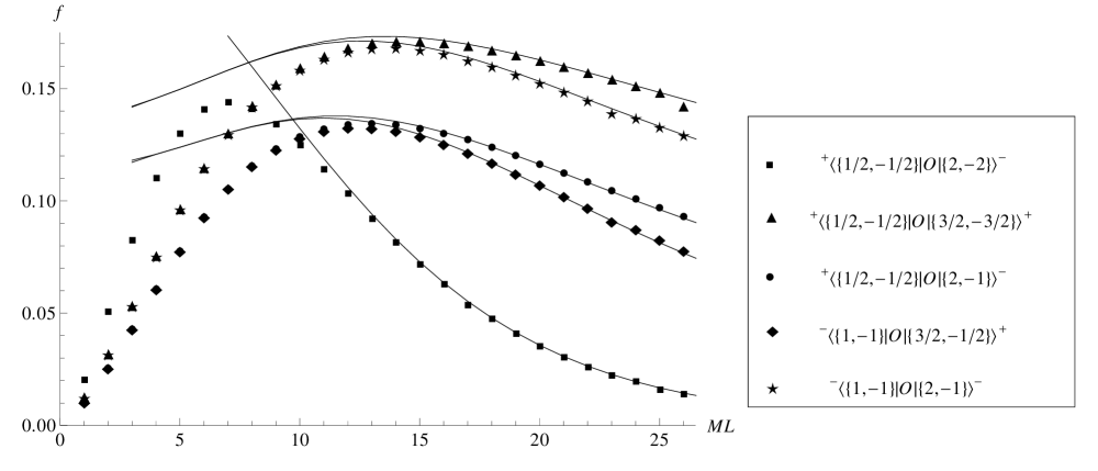
Figure 4.1: Non-diagonal form factors in the $Q=0$ sector for $\xi=50/239$. A few examples of individual data points affected by truncation effects magnified by the vicinity of a level crossing can be seen at $ML=23$, cf. the second and fourth lines from below (plotted with diamonds and stars, respectively).

In addition we can use the soliton-soliton two-particle states. For off-diagonal matrix elements it is straightforward to use (3.10) and we obtained a good agreement as demonstrated in fig. 4.2. For the diagonal case however, one observes a discrepancy between the predictions from eqn. (3.3) and the numerical results in fig. 4.3 which becomes smaller for smaller values of $\xi$. As illustrated in fig. 4.4, this can be explained by truncation errors, which are indeed improved by decreasing $\xi$. One can try to extrapolate the truncation dependence; however, it turns out that it does not fit the theoretically expected asymptotics derived in [49], which means that the leading order renormalization group behaviour is not yet valid at the cutoffs considered. Extrapolations reproducing the theoretical predictions can be found, but for a cut-off dependence which has an exponent that differs from the predictions of the renormalization group; in addition, the available range of cutoff values is not sufficient for a reliable determination of the exponent from the numerical data. In the conclusions we discuss how the situation can be improved, but this is out of the scope of the present work.

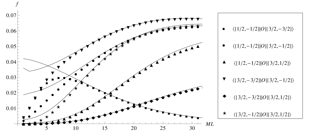
Figure 4.2: Non-diagonal form factors in the $Q=2$ sector for $\xi=50/239$

$\xi=2/7$

$\xi=50/239$

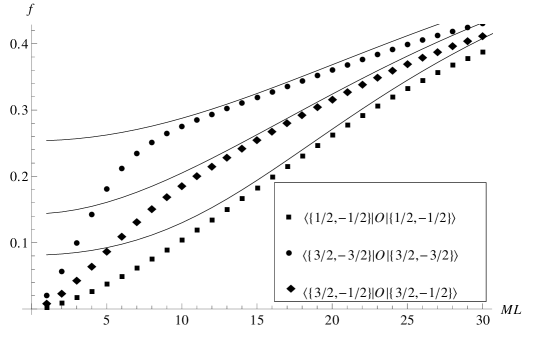
$\xi=50/311$

Figure 4.3: Diagonal form factors in the $Q=2$ sector

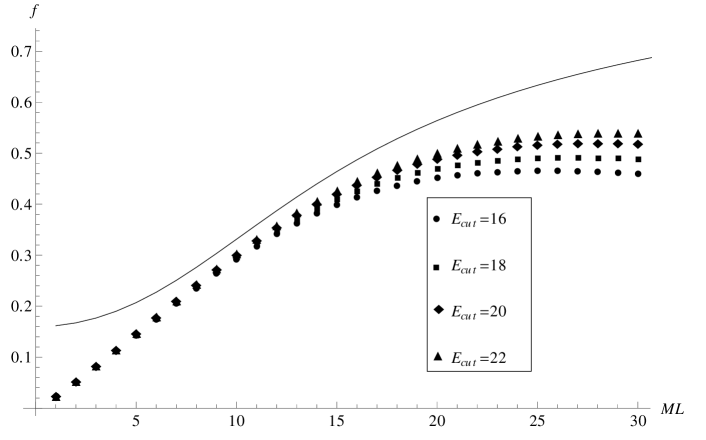
Figure 4.4: Truncation dependence of the diagonal matrix element $\langle\{1/2,-1/2\}|\mathcal{O}|\{1/2,-1/2\}\rangle$ in the $Q=2$ sector for $\xi=2/7$

4.4 Six-soliton form factors

We tested six-soliton form factors by comparing the predictions from eqn. (3.10) to off-diagonal matrix elements between states composed of three solitons (and no antisolitons). The agreement is again very convincing, as demonstrated in fig. 4.5. For diagonal matrix elements, we noticed similar discrepancies as in the case of diagonal four-soliton form factors; however, the truncation dependence proved to be much worse in this case, so while the results were qualitatively consistent, they were not as good as for the four-soliton case.

In addition, for this case there is an interesting new possibility of having disconnected parts originating from particles with exactly zero rapidity, described by eqn. (3.12). For these matrix elements we get a very convincing agreement again, as demonstrated in fig. 4.6.

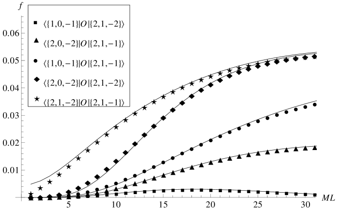
Figure 4.5: Off-diagonal form factors in the $Q=3$ sector for $\xi=50/239$

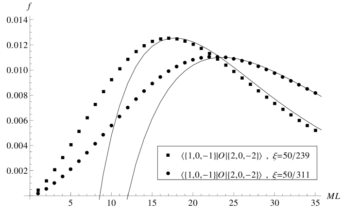
Figure 4.6: Form factors with zero-momentum disconnected pieces in the $Q=3$ sector

5 Conclusions and outlook

In this work we compared the conjectured exact soliton form factors of sine-Gordon theory, obtained from the bootstrap, to finite volume matrix elements given by the truncated conformal space approach.

For non-diagonal matrix elements we find excellent agreement between the numerical results and theoretical expectations, both for four-soliton and six-soliton form factors. For diagonal matrix elements we found some discrepancy similar to the one noticed in [28] for four-breather form factors. This discrepancy tends to decrease for smaller value of $\xi$ (or equivalently $\beta$) and we argued that it can be attributed to truncation effects. Similar effects were observed for boundary form factors in [51] and based on the accumulated data we are inclined to think that there is something special about cutoff dependence of diagonal matrix elements.

Convergence of the TCSA can be improved by renormalization group methods [48, 49, 50]; as we discussed in subsection 4.3 it turns out that the TCSA data are not yet in the regime where the leading RG behaviour is applicable, and the extrapolation fits are not reliable enough to determine the exponent of the cutoff dependence. This can be helped by applying the numerical RG technique proposed in [49]; however, developing a systematic program for that takes a substantial amount of effort and time, and work in this direction has just started. One can also extend the domain of comparison by improving the theoretical description for smaller volumes (where truncation errors are negligible) by describing exponential finite size effects.

Aside from the above-mentioned technical issues, there is a crucial missing piece, namely the description of disconnected pieces for states in which the scattering is non-diagonal, i.e. an extension of formulae (3.3, 3.12) to the general case. The work aimed at resolving this issue is in progress, and the developments in this paper are also useful in preparing a testing ground for future theoretical conjectures. Once this final piece is in place, it will be possible to use the systematic formalism developed in [35] for the form factor expansion of finite temperature correlators to evaluate correlators in field theories with non-diagonal scattering, such as sine-Gordon theory or the O(3) nonlinear $\sigma$-model.

Appendix A Explicit formulae for the soliton form factors

Let us denote the form factor functions defined by Lukyanov by

$$\mathcal{F}_{\sigma_{2n}\dots\sigma_{1}}^{(a)}(\theta_{2n},\dots,\theta_{1})=\mathcal{G}_{a}(\beta)\langle\langle Z_{\sigma_{2n}}(\theta_{2n})\dots Z_{\sigma_{1}}(\theta_{1})\rangle\rangle$$

where $\sigma_{i}=\pm$ and

$$\sum_{k=1}^{2n}\sigma_{k}=0$$

is necessary for the matrix element to be different from zero. The operators $Z$ are given by

$$Z_{+}(\theta) = \sqrt{i\frac{\mathcal{C}_{2}}{4\mathcal{C}_{1}}}\mathrm{e}^{a\theta}\mathrm{e}^{i\phi(\theta)}$$

$$Z_{-}(\theta) = \sqrt{i\frac{\mathcal{C}_{2}}{4\mathcal{C}_{1}}}\mathrm{e}^{-a\theta}\Bigg{\{}\mathrm{e}^{\frac{i4\pi^{2}}{\beta^{2}}}\int_{C_{+}}\frac{d\gamma}{2\pi}\mathrm{e}^{(1-2a-8\pi/\beta^{2})(\gamma-\theta)}\mathrm{e}^{-i\bar{\phi}(\gamma)}\mathrm{e}^{i\phi(\theta)}$$

$$-\mathrm{e}^{-\frac{i4\pi^{2}}{\beta^{2}}}\int_{C_{-}}\frac{d\gamma}{2\pi}\mathrm{e}^{(1-2a-8\pi/\beta^{2})(\gamma-\theta)}\mathrm{e}^{i\phi(\theta)}\mathrm{e}^{-i\bar{\phi}(\gamma)}\Bigg{\}}$$

The averages are computed by the multiplicative Wick theorem (valid for exponential operators) using

$$\langle\langle\mathrm{e}^{i\phi(\theta_{2})}\mathrm{e}^{i\phi(\theta_{1})}\rangle\rangle = G(\theta_{1}-\theta_{2})$$

$$\langle\langle\mathrm{e}^{i\phi(\theta_{2})}\mathrm{e}^{i\bar{\phi}(\theta_{1})}\rangle\rangle = W(\theta_{1}-\theta_{2})$$

$$\langle\langle\mathrm{e}^{i\bar{\phi}(\theta_{2})}\mathrm{e}^{i\bar{\phi}(\theta_{1})}\rangle\rangle = \bar{G}(\theta_{1}-\theta_{2})$$

The function $G$ is given by the integral representation

$$G(\theta) = i\mathcal{C}_{1}\sinh\left(\frac{\theta}{2}\right)\exp\left\{\int_{0}^{\infty}\frac{dt}{t}\sinh^{2}\left(\left(1-\frac{i\theta}{\pi}\right)t\right)\frac{\sinh t\left(\xi-1\right)}{\sinh 2t\cosh t\sinh t\xi}\right\}$$

$$= i\mathcal{C}_{1}\sinh\left(\frac{\theta}{2}\right)\prod_{k=1}^{N}g(\theta,\xi,k)^{k}\,\exp\Bigg{\{}\int_{0}^{\infty}\frac{dt}{t}\mathrm{e}^{-4Nt}\left(1+N-N\,\mathrm{e^{-4t}}\right)$$

$$\times\sinh^{2}\left(\left(1-\frac{i\theta}{\pi}\right)t\right)\frac{\sinh t\left(\xi-1\right)}{\sinh 2t\cosh t\sinh t\xi}\Bigg{\}}$$

where the second formula provides an extension for the domain of convergence of the integral by factorizing out the following pole factors

$$g(\theta,\xi,k) = \frac{\Gamma\left(\frac{(2k+1+\xi)\pi-i\theta}{\pi\xi}\right)\Gamma\left(\frac{2k+1}{\xi}\right)^{2}\Gamma\left(\frac{(2k+1)\pi-i\theta}{\pi\xi}\right)}{\Gamma\left(\frac{2k+\xi}{\xi}\right)^{2}\Gamma\left(\frac{(2k+\xi)\pi-i\theta}{\pi\xi}\right)\Gamma\left(\frac{(2k-2+\xi)\pi+i\theta}{\pi\xi}\right)}$$

$$\times\frac{\Gamma\left(\frac{(2k-1)\pi+i\theta}{\pi\xi}\right)\Gamma\left(\frac{2k-1+\xi}{\xi}\right)^{2}\Gamma\left(\frac{(2k-1+\xi)\pi+i\theta}{\pi\xi}\right)}{\Gamma\left(\frac{2k}{\xi}\right)^{2}\Gamma\left(\frac{(2k+2)\pi-i\theta}{\pi\xi}\right)\Gamma\left(\frac{2k\pi+i\theta}{\pi\xi}\right)}$$

and is independent of $N$,

$$\mathcal{C}_{1} = G(-i\pi)=\exp\left\{-\int_{0}^{\infty}\frac{dt}{t}\frac{\sinh^{2}(t/2)\sinh(t(\xi-1))}{\sinh(2t)\cosh(t)\sinh(t\xi)}\right\}$$

$$\mathcal{C}_{2} = \exp\left\{4\int_{0}^{\infty}\frac{dt}{t}\frac{\sinh^{2}(t/2)\sinh(t(\xi-1))}{\sinh(2t)\sinh(t\xi)}\right\}$$

and

$$W(\theta) = \frac{1}{G(\theta+i\pi/2)G(\theta-i\pi/2)}$$

$$= -\frac{2}{\cosh\theta}\prod_{k=1}^{N}\frac{\Gamma\left(\frac{(2k-5/2+\pi)\xi+i\theta}{\pi\xi}\right)\Gamma\left(\frac{(2k-1/2)\pi-i\theta}{\pi\xi}\right)\Gamma\left(\frac{2k-1/2}{\xi}\right)^{2}}{\Gamma\left(1+\frac{2k-3/2}{\xi}\right)^{2}\Gamma\left(\frac{(2k+1/2)\pi-i\theta}{\pi\xi}\right)\Gamma\left(\frac{(2k-3/2)\pi+i\theta}{\pi\xi}\right)}$$

$$\times\exp\left\{-2\int_{0}^{\infty}\frac{dt}{t}\mathrm{e}^{-4Nt}\sinh^{2}\left(\left(1-\frac{i\theta}{\pi}\right)t\right)\frac{\sinh t\left(\xi-1\right)}{\sinh 2t\sinh t\xi}\right\}$$

$$\bar{G}(\theta) = \frac{1}{W(\theta+i\pi/2)W(\theta-i\pi/2)}$$

$$= -\frac{\mathcal{C}_{2}}{4}\xi\sinh\frac{\theta+i\pi}{\xi}\sinh\theta$$

where, again, the integral formula is eventually independent of the natural number $N$; it provides a representation which converges faster numerically and is valid further away from the real $\theta$ axis with increasing $N$. The contours in the integrals are such that the “principal poles” of the $W$-functions are always between the contour and the real line, where the “principal pole” of $W(x)$ is the one located at $x=-i\pi/2$.

The integral representation can be evaluated in a closed form at the free fermion point $\xi=1$ and also for the two-particle case when $a$ is either integer or half-integer [42]. Here we only quote the case needed in the text:

$$\mathcal{F}_{\pm\mp}^{1}(\theta)=\mathcal{G}_{1}(\beta)\,\frac{G(\theta)}{G(-i\pi)}\cot\left(\frac{\pi\xi}{2}\right)\frac{4i\cosh\left(\frac{\theta}{2}\right)\mathrm{e}^{\mp\frac{\theta+i\pi}{2\xi}}}{\xi\sinh\left(\frac{\theta+i\pi}{\xi}\right)}$$ (A.1)

The numerical evaluation of the integral representation is rather involved; the details are given in [32].

Acknowledgments

This work was partially supported by the Hungarian OTKA grant K75172.

Dedication

This paper is dedicated to Zalán Horváth, my former MSc and PhD supervisor and long-time mentor, who recently passed away. It was under his supervision that I learned about the form factor bootstrap [52, 53], more specifically about the sine-Gordon form factors studied in this work. He was interested in finding a direct way to establish that the exact form factors really give a solution to the quantum field theory dynamics, which is one of the outcomes of this paper and much of my recent work.

Gábor Takács

References

- [1] A. B. Zamolodchikov and A. B. Zamolodchikov, “Factorized S-matrices in two dimensions as the exact solutions of certain relativistic quantum field models,” Annals Phys. 120 (1979) 253–291.
- [2] G. Mussardo, “Off critical statistical models: Factorized scattering theories and bootstrap program,” Phys. Rept. 218 (1992) 215–379.
- [3] M. Karowski and P. Weisz, “Exact Form-Factors in (1+1)-Dimensional Field Theoretic Models with Soliton Behavior,” Nucl. Phys. B139 (1978) 455.
- [4] A. N. Kirillov and F. A. Smirnov, “A representation of the current algebra connected with the SU(2) invariant Thirring model,” Phys. Lett. B198 (1987) 506–510.
- [5] F. A. Smirnov, “Form-factors in completely integrable models of quantum field theory,” Adv. Ser. Math. Phys. 14 (1992) 1–208.
- [6] Z. Bajnok, L. Palla, and G. Takacs, “On the boundary form factor program,” Nucl. Phys. B750 (2006) 179–212, arXiv:hep-th/0603171.
- [7] G. Takacs, “Form factors of boundary exponential operators in the sinh-Gordon model,” Nucl. Phys. B801 (2008) 187–206, arXiv:0801.0962.
- [8] J. L. Cardy and G. Mussardo, “Form-factors of descendent operators in perturbed conformal field theories,” Nucl.Phys. B340 (1990) 387–402.
- [9] A. Koubek and G. Mussardo, “On the operator content of the sinh-Gordon model,” Phys. Lett. B311 (1993) 193–201, arXiv:hep-th/9306044.
- [10] A. Koubek, “A Method to determine the operator content of perturbed conformal field theories,” Phys. Lett. B346 (1995) 275–283, arXiv:hep-th/9501028.
- [11] A. Koubek, “Form-factor bootstrap and the operator content of perturbed minimal models,” Nucl. Phys. B428 (1994) 655–680, arXiv:hep-th/9405014.
- [12] A. Koubek, “The Space of local operators in perturbed conformal field theories,” Nucl. Phys. B435 (1995) 703–734, arXiv:hep-th/9501029.
- [13] F. A. Smirnov, “Counting the local fields in SG theory,” Nucl. Phys. B453 (1995) 807–824, arXiv:hep-th/9501059.
- [14] G. Delfino and G. Mussardo, “The spin-spin correlation function in the two-dimensional Ising model in a magnetic field at ,” Nucl.Phys. B455 (1995) 724–758, arXiv:hep-th/9507010 [hep-th].
- [15] G. Delfino and G. Niccoli, “Isomorphism of critical and off-critical operator spaces in two-dimensional quantum field theory,” Nucl.Phys. B799 (2008) 364–378, arXiv:0712.2165 [hep-th].
- [16] V. P. Yurov and A. B. Zamolodchikov, “Correlation functions of integrable 2-D models of relativistic field theory. Ising model,” Int. J. Mod. Phys. A6 (1991) 3419–3440.
- [17] A. B. Zamolodchikov, “Two point correlation function in scaling Lee-Yang model,” Nucl. Phys. B348 (1991) 619–641.
- [18] A. B. Zamolodchikov, “Irreversibility of the Flux of the Renormalization Group in a 2D Field Theory,” JETP Lett. 43 (1986) 730–732.
- [19] G. Delfino, P. Simonetti, and J. L. Cardy, “Asymptotic factorisation of form factors in two- dimensional quantum field theory,” Phys. Lett. B387 (1996) 327–333, arXiv:hep-th/9607046.
- [20] B. Pozsgay and G. Takacs, “Form factors in finite volume I: form factor bootstrap and truncated conformal space,” Nucl. Phys. B788 (2008) 167–208, arXiv:0706.1445.
- [21] B. Pozsgay and G. Takacs, “Form factors in finite volume II:disconnected terms and finite temperature correlators,” Nucl. Phys. B788 (2008) 209–251, arXiv:0706.3605.
- [22] F. A. Smirnov, “Quasi-classical study of form factors in finite volume,” arXiv:hep-th/9802132.
- [23] V. E. Korepin and N. A. Slavnov, “Form Factors in the Finite Volume,” International Journal of Modern Physics B 13 (1999) 2933–2941, arXiv:math-ph/9812026.
- [24] G. Mussardo, V. Riva, and G. Sotkov, “Finite-volume form factors in semiclassical approximation,” Nucl. Phys. B670 (2003) 464–478, arXiv:hep-th/0307125.
- [25] B. Doyon, “Finite-temperature form factors: A review,” SIGMA 3 (2007) 011, arXiv:hep-th/0611066.
- [26] B. Pozsgay, “Finite volume form factors and correlation functions at finite temperature,” arXiv:0907.4306 [hep-th].
- [27] M. Kormos and G. Takacs, “Boundary form factors in finite volume,” Nucl. Phys. B803 (2008) 277–298, arXiv:0712.1886.
- [28] G. Feher and G. Takacs, “Sine-Gordon form factors in finite volume,” Nucl.Phys. B852 (2011) 441–467, arXiv:1106.1901 [hep-th].
- [29] G. Takacs, “Determining matrix elements and resonance widths from finite volume: the dangerous -terms,” JHEP 1111 (2011) 113, arXiv:1110.2181 [hep-th].
- [30] B. Pozsgay and G. Takacs, “Characterization of resonances using finite size effects,” Nucl. Phys. B748 (2006) 485–523, arXiv:hep-th/0604022.
- [31] G. Takacs, “Form factor perturbation theory from finite volume,” Nucl. Phys. B825 (2010) 466–481, arXiv:0907.2109.
- [32] T. Palmai, “Regularization of multi-soliton form factors in sine-Gordon model,” arXiv:1111.7086 [math-ph].
- [33] F. H. L. Essler and R. M. Konik, “Applications of massive integrable quantum field theories to problems in condensed matter physics,” arXiv:cond-mat/0412421.
- [34] F. H. L. Essler and R. M. Konik, “Finite-temperature dynamical correlations in massive integrable quantum field theories,” J. Stat. Mech. 0909 (2009) P09018, arXiv:0907.0779 [cond-mat.str-el].
- [35] B. Pozsgay and G. Takacs, “Form factor expansion for thermal correlators,” J. Stat. Mech. 1011 (2010) P11012, arXiv:1008.3810.
- [36] F. H. L. Essler and R. M. Konik, “Finite-temperature lineshapes in gapped quantum spin chains,” Phys. Rev. B78 (2008) 100403, arXiv:0711.2524 [cond-mat.str-el].
- [37] M. Kormos and B. Pozsgay, “One-Point Functions in Massive Integrable QFT with Boundaries,” JHEP 1004 (2010) 112, arXiv:1002.2783 [hep-th].
- [38] V. P. Yurov and A. B. Zamolodchikov, “Truncated conformal space approach to scaling Lee-Yang model,” Int. J. Mod. Phys. A5 (1990) 3221–3246.
- [39] G. Feverati, F. Ravanini, and G. Takacs, “Truncated conformal space at c = 1, nonlinear integral equation and quantization rules for multi-soliton states,” Phys. Lett. B430 (1998) 264–273, arXiv:hep-th/9803104.
- [40] F. A. Smirnov, “Form-factors in completely integrable models of quantum field theory,” Adv. Ser. Math. Phys. 14 (1992) 1–208.
- [41] S. L. Lukyanov, “Free field representation for massive integrable models,” Commun. Math. Phys. 167 (1995) 183–226, arXiv:hep-th/9307196.
- [42] S. L. Lukyanov, “Form factors of exponential fields in the sine-Gordon model,” Mod. Phys. Lett. A12 (1997) 2543–2550, arXiv:hep-th/9703190.
- [43] H. M. Babujian, A. Fring, M. Karowski, and A. Zapletal, “Exact form factors in integrable quantum field theories: The sine-Gordon model,” Nucl. Phys. B538 (1999) 535–586, arXiv:hep-th/9805185.
- [44] H. Babujian and M. Karowski, “Exact form factors in integrable quantum field theories: The sine-Gordon model. II,” Nucl. Phys. B620 (2002) 407–455, arXiv:hep-th/0105178.
- [45] S. L. Lukyanov and A. B. Zamolodchikov, “Exact expectation values of local fields in quantum sine-Gordon model,” Nucl. Phys. B493 (1997) 571–587, arXiv:hep-th/9611238.
- [46] A. B. Zamolodchikov, “Mass scale in the sine-Gordon model and its reductions,” Int. J. Mod. Phys. A10 (1995) 1125–1150.
- [47] B. Pozsgay, “Luscher’s mu-term and finite volume bootstrap principle for scattering states and form factors,” Nucl. Phys. B802 (2008) 435–457, arXiv:0803.4445 [hep-th].
- [48] G. Feverati, K. Graham, P. A. Pearce, G. Z. Toth, and G. Watts, “A Renormalisation group for TCSA,” arXiv:hep-th/0612203 [hep-th].
- [49] R. M. Konik and Y. Adamov, “A Numerical Renormalization Group for Continuum One-Dimensional Systems,” Phys. Rev. Lett. 98 (2007) 147205, arXiv:cond-mat/0701605 [cond-mat.str-el].
- [50] P. Giokas and G. Watts, “The renormalisation group for the truncated conformal space approach on the cylinder,” arXiv:1106.2448 [hep-th].
- [51] M. Lencses and G. Takacs, “Breather boundary form factors in sine-Gordon theory,” Nucl.Phys. B852 (2011) 615–633, arXiv:1106.1902 [hep-th].
- [52] Z. Horvath and G. Takacs, “Free field representation for the O(3) nonlinear sigma model and bootstrap fusion,” Phys. Rev. D51 (1995) 2922–2932, arXiv:hep-th/9501006.
- [53] Z. Horvath and G. Takacs, “Form-factors of the sausage model obtained with bootstrap fusion from sine-Gordon theory,” Phys. Rev. D53 (1996) 3272–3284, arXiv:hep-th/9601040.