Many-body effects in magnetic inelastic electron tunneling spectroscopy

Abstract

Magnetic inelastic electron tunneling spectroscopy (IETS) shows sharp increases in conductance when a new conductance channel associated to a change in magnetic structure is open. Typically, the magnetic moment carried by an adsorbate can be changed by collision with a tunneling electron; in this process the spin of the electron can flip or not. A previous one-electron theory [Phys. Rev. Lett. 103, 176601 (2009)] successfully explained both the conductance thresholds and the magnitude of the conductance variation. The elastic spin flip of conduction electrons by a magnetic impurity leads to the well known Kondo effect. In the present work, we compare the theoretical predictions for inelastic magnetic tunneling obtained with a one-electron approach and with a many-body theory including Kondo-like phenomena. We apply our theories to a singlet-triplet transition model system that contains most of the characteristics revealed in magnetic IETS. We use two self-consistent treatments (non-crossing approximation and self-consistent ladder approximation). We show that, although the one-electron limit is properly recovered, new intrinsic many-body features appear. In particular, sharp peaks appear close to the inelastic thresholds; these are not localized exactly at thresholds and could influence the determination of magnetic structures from IETS experiments.Analysis of the evolution with temperature reveals that these many-body features involve an energy scale different from that of the usual Kondo peaks. Indeed, the many-body features perdure at temperatures much larger than the one given by the Kondo energy scale of the system.

I Introduction

Magnetic inelastic electron tunneling spectroscopy (magnetic IETS) detects magnetic excitations on a surface by measuring the changes of conductance of a scanning tunneling micrsocope (STM) junction when an excitation is produced Heinrich et al. (2004). As in general IETS, the possibility to excite the surface leads to an increase of the number of possible final channels for the tunneling electron when the junction bias matches an excitation energy threshold, consequently leading to an abrupt increase of the junction conductance. This high sensitivity on the small magnetic energy scale has permitted Hirjibehedin and coworkers Hirjibehedin et al. (2007) to measure the magnetic anisotropy energy (MAE) of single atomic adsorbates as well as the magnetic coupling among them Hirjibehedin et al. (2006). More recent experiments revealed the change of sign of MAE when a phthalocyanine molecule is adsorbed on a surface Tsukahara et al. (2009) and the existence of an exchange coupling between magnetic molecules in a multilayer setup Chen et al. (2008). This technique has open a venue to the study of magnetic phenomena at surfaces on the single atom or molecule scale.

Theories have been developed to rationalize the steps in conductance found in magnetic IETS with a good degree of success Fransson (2009); Fernández-Rossier (2009); Persson (2009); Lorente and Gauyacq (2009). The large changes in conductance observed in magnetic IETS were explained by the large parent coefficients of the initial and final adsorbate states in the tunneling state  Lorente and Gauyacq (2009). During tunneling the spins of the tunneling electron and of the magnetic adsorbate couple together into a total spin $S_{T}$ that characterizes the spin symmetry of the tunneling process. The excitation process is then pictured as the coupling/decoupling of the two spins. Since the parentage coefficients of the $S_{T}$ states in the initial and final magnetic states of the adsorbate can be large (these are Clebsch-Gordan coefficients associated to MAE structure coefficients), the probability of forming various excited final states can be very large. In this way, the flux of incident electrons is shared among the possible final channels that are energetically possible; the branching ratios among channels are simply governed by structure coefficients. This theory also showed that the magnetic excitation of an adsorbate may or may not imply spin-flip of the tunneling electron Lorente and Gauyacq (2009).

The Kondo effect is associated with a phenomenon bearing many links with magnetic IETS: the fluctuations induced by the spin-flip of an electron during its collision with a magnetic impurity at constant energy. Kondo physics and inelastic effects have been extensively studied in quantum dots and nanotubes Inoshita et al. (1993, 1997); Liang et al. (2002); Nygard et al. (2000); Kogan et al. (2003); Paaske et al. (2006). Recently, vibrational side-bands have been predicted and reported for molecules displaying Kondo peaks at zero bias Cornaglia et al. (2004); Paaske and Flensberg (2005); Parks et al. (2007); Cornaglia et al. (2007); Fernández-Torrente et al. (2008). Inelastic processes in Kondo physics have been studied by Zarand, Borda and coworkers Zaránd et al. (2004); Borda et al. (2007) who have shown that the usual Kondo theories can reveal the amount of elastic and inelastic spin-flip in the electron-impurity scattering event. For the particular case of magnetic IETS, Zitko and Pruschke Zitko and Pruschke (2010) have applied Kondo theories to the study of the coexistence of a Kondo peak and of IETS steps in the STM conductance of Co atoms on CuN/Cu(100) substrates. Unfortunately, the numerical renormalization group method that was used is not very accurate in reproducing the sharp conductance steps. However, these authors gave the first unified picture of Kondo and magnetic IETS.

More recently, Hurley and collaborators Hurley et al. (2011) have used the Kondo Hamiltonian and perturbation theory to analyze the magnetic IETS of Co and Fe on CuN/Cu(100). The authors conclude that certain spike-like structures at the inelastic thresholds in experimental IETS are actually due to a Kondo-like effect. However, spike-like structures close to the inelastic thresholds can also be found due to electronic heating under high current conditions as recent experimental and theoretical reports Loth et al. (2010); Delgado and Fernandez-Rossier (2010); Novaes et al. (2010) show. Indeed, the conductance changes in a non-linear way if a tunneling electron probes the adsorbate still excited by earlier tunneling electrons.

Here, we study the magnetic transitions between singlet and triplet configurations of a magnetic adsorbate. We use our previous study on adsorbed copper phthalocyanine Korytár and Lorente (2011) and parametrize it to study the role of different ingredients in the spectral function. Our study considers two independent spins localized in two different molecular orbitals whose interaction is simply given by a Heisenberg term of exchange interaction $I$. This model contains similar physics to the recent two-impurity Kondo system studied by Bork and co-workers Bork et al. (2011).

In the first part of this work, we use our previous one-electron theory Lorente and Gauyacq (2009) to evaluate the magnetic IETS for a singlet-triplet excitation. In the second part, we use the non-crossing approximation Korytár and Lorente (2011) and the self-consistent ladder approximation Maekawa et al. (1985) for the same model system. The sharp behavior of the conductance steps due to IETS is accounted for by both theories. However, many-body effects appear to be very important at the inelastic thresholds. Depending on the parameters of the impurity, we further find that the actual excitation thresholds can be substantially shifted when many-body effects are included. This finding can have important consequences in the determination of MAE and more generally of adsorbate magnetic structures from IETS.

II One-electron theory

The magnetic excitation of magnetic impurities on a solid surface using an STM was modelled as an electron-impurity collision in Refs. [Lorente and Gauyacq, 2009; Gauyacq et al., 2010; Novaes et al., 2010]. During the collision of the electron with the impurity, the tunneling electron and adsorbate spins briefly couple together. A transient resonant state with a finite lifetime can be involved, but not necessarily; it could simply be a scattering state that fixes the tunneling symmetries. These symmetries depend on both the electron energy and the electronic structure of the impurity. In the present case, the electron energy is very small since typical magnetic excitations are in the meV range. Hence, the impurity’s electronic structure at the Fermi energy is the relevant one during the collision. In Refs. [Lorente and Gauyacq, 2009; Gauyacq et al., 2010; Novaes et al., 2010] the impurities had orbitals straddling the Fermi energy of the substrate which were thus involved in the tunneling process.

In the present work, we extend the study to systems where a positive ion is a more likely origin of the transient state. In particular, we are studying the singlet-triplet excitations of a magnetic impurity with a large charging energy $U$. In this case, the negative ion is energetically less accessible than the positive one. This feature has been used to model the Kondo effect in certain molecular systems Roura Bas and Aligia (2009); Bas and Aligia (2010); Cornaglia et al. (2011); Korytár and Lorente (2011).

The modelling of the Kondo effect runs parallel to the one-electron theory used to account for magnetic excitations in impurities. Indeed, the Kondo effect (see for example Ref. [Korytár and Lorente, 2011] and references therein) can be described as a fluctuation between a charged transient state and the ground state of the impurity. The Kondo effect builds up on the coherence between impinging electrons, it is a genuine many-body effect, while our earlier IETS studies Lorente and Gauyacq (2009); Gauyacq et al. (2010); Novaes et al. (2010) only consider single-electron collisions.

Both in the one-electron and many-body pictures, the tunneling state connects the initial state of the impurity with a final state that can be different, leading to magnetic excitations. We study below how many-body effects influence magnetic excitation processes.

II.1 Inelastic transition rate

We assume the tunneling process (electron-adsorbate collision) to be very fast, much faster than the interaction at play in the singlet-triplet splitting, so that we can resort to the sudden approximation. The $T$-matrix Gauyacq et al. (2010); Novaes et al. (2010) between an initial state $|i\rangle$ and a final state $|f\rangle$ of the complete electron+adsorbate system is obtained from the sudden $T$-matrix expressed in the basis set of the intermediate states $|S_{T},M_{T}\rangle$ (spherical spin symmetry is kept during the brief collision). In the present case, since the system ground state is a singlet, the tunneling symmetry can only be $S_{T}$=1/2.

In the large $U$ limit, the collision takes place between a hole and the impurity. The ground state of the molecule is a singlet, then the initial state is a singlet times (tensorial product) a hole of the conduction band. Hence,

$$|i\rangle=\hat{c}_{\sigma}|0,0\rangle$$ (1)

where $\hat{c}_{\sigma}$ destroys an electron with spin $\sigma$, and the impurity in the ground state is given by its spin $|S,M\rangle$ which is a singlet $|0,0\rangle$ . Similarly, the final state is

$$|f\rangle=\hat{c}_{\sigma^{\prime}}|S,M\rangle$$ (2)

where the impurity is left in one of the $|S,M\rangle$ states and the hole is in a $\sigma^{\prime}$ state. Below, we assume the STM tip to be unpolarized, so that we sum over the contributions for $\sigma$ and $\sigma^{\prime}$ spins.

The sudden $T$-matrix reduces to a projection operator on all the $|S_{T},M_{T}\rangle$ states times a common transmission amplitude, $B$ Lorente and Gauyacq (2009); Gauyacq et al. (2010). In tunneling, the transmission probability density is proportional to the density of states of the sample, $\rho(\omega)$. This still holds in more complicated situations as shown in Ref. [Meir and Wingreen, 1992]. Then, the transmission probability density is proportional to a constant coming from the transmission amplitude, $|B|^{2}$, times the density of states. Hence, the elastic probability density for an electron energy $\omega$, $T_{e}$, is given by

$$T_{e}(\omega)=\rho(\omega)\sum_{\sigma}|\sum_{M_{T}}|B\langle S_{T},M_{T}|\hat{c}_{\sigma}|0,0\rangle|^{2}|^{2}=\frac{|B|^{2}\rho(\omega)}{2}.$$ (3)

The inelastic contribution, $T_{i}$, contains three possible orientations, $M_{f}$, of the impurity’s spin because it is a triplet. Hence,

$$T_{i}(\omega) = \rho(\omega)\sum_{\sigma,\sigma^{\prime},M_{f}}|\sum_{M_{T}}B\langle 0,0|\hat{c}^{\dagger}_{\sigma}|S_{T},M_{T}\rangle$$ (4)

$$\times \langle S_{T},M_{T}|\hat{c}_{\sigma^{\prime}}|1,M_{f}\rangle|^{2}$$

$$= \frac{3|B|^{2}\rho(\omega)}{2}.$$

At this point, we can stress that the inelastic conductance is associated to both spin-flip ($\sigma$ $\neq$ $\sigma^{\prime}$) and non spin-flip ($\sigma$ $=$ $\sigma^{\prime}$) processes for the tunneling electron; excitation of the triplet state by a tunneling electron without a change of the electron spin is 50 % less probable than excitation of a triplet adsorbate state with a spin-flip of the tunneling electron.

From Eqs. (3) and (4) the relative contribution of the elastic part to the transmision probability density at an inelastic threshold is just

$$\frac{T_{e}}{T_{e}+T_{i}}=\frac{1}{4}$$ (5)

and 3/4 is the relative contribution of the inelastic part of the transmission probability density.

In the spirit of the generalization of the Landauer transmission formula to include inelastic transitions Meir and Wingreen (1992); Ness (2006); Monturet and Lorente (2008), it is possible to link Meir and Wingreen (1992) the transmission probability density to the projected density of states on the magnetic adsorbate or spectral function, $A$, and we use, below, this link to compare the results of the one-electron and many-body studies. In the present one-electron approach, the spectral function, $A$, is obtained as:

$$A=\rho(\omega)\{\frac{1}{4}+\frac{3}{4}[f(\omega+I)+f(I-\omega)]\},$$ (6)

where $I$ is the singlet-triplet excitation energy and $f(\omega)$ is the Fermi function of the substrate.

Fig. 1 shows the characteristic step-like function for the spectral function, $A$, at low temperature. The two steps at positive and negative energy are associated to the opening of the inelastic triplet channel. The results in Fig. 1 use the parameterization of the adsorbed CuPc molecule determined in Ref. Korytár and Lorente, 2011, in particular the excitation energy, $I$, is equal to 25 meV.

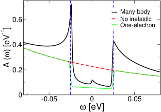
Figure 1: Projected density of states on the magnetic adsorbate electronic structure or spectral function $A$ as a function of the electron energy $\omega$ with respect to the Fermi energy of the substrate. The vertical dashed lines show the one-electron inelastic thresholds. The figure presents the adsorbate density of states in the absence of inelastic effects (marked as “No inelastic”), the many-body spectral function and the one-electron conductance with inelastic effects. The system’s temperature is 7 K.

II.2 Thermal effects

The above one-electron results in Fig. 1 correspond to a low temperature of the surface. Thermal effects tend to wash out the inelastic structures via two contributions: i) the Fermi function is not a step function and this rounds the conductance steps at threshold and ii) at equilibrium at finite temperature, the system is not initially entirely in the singlet state, a small thermal population of the triplet is also present.

For the finite-temperature differential conductance, the first effect has been discussed in detail in Refs. Lauhon and Ho (2001); Lambe and Jaklevic (1968). The abrupt steps at inelastic thresholds that are present in the conductance at vanishing temperature are replaced by rounded steps due to the smearing of the energy distribution of the electrons at finite temperature. This leads to a significant broadening of the step function of the order of 5.5 $k_{B}T$ Lauhon and Ho (2001). In the present one-electron results however, for a consistent comparison with the many body results on the spectral function, we evaluate the above one-electron spectral function, i.e. we do not include the broadening effect coming from the thermal distribution of the electrons in the tip.

The second effect is due to the finite thermal population of the triplet state by the Boltzman factor, $F=\exp[-I/k_{B}T]$ and the corresponding decrease of the singlet population. The total spectral function, $A$, is then equal to:

$$A = \{\frac{1}{4}+\frac{3}{4}[f(\omega+I)+f(I-\omega)]\}\frac{\rho(\omega)}{1+3F}$$ (7)

$$+ \frac{3F\rho(\omega)}{1+3F}$$

Note the factor 3 due to the triplet degeneracy. The total (elastic + inelastic) contributions of the singlet and triplet states are equal. Since the triplet contribution does not exhibit any step, the thermal population of the triplet state tends to smooth out the stepped structure. This effect is only visible on the results in Fig. 2 at the highest temperature.

III Many-body theory

The extension of the above one-electron theory to the many-body case is achieved by keeping the coherence between impinging holes. This is a tremendous task, but can be easily achieved using self-consistent schemes such as the non-crossing approximation (NCA) and the self-consistent ladder approximation (SCLA).

III.1 Non-crossing approximation: Anderson Hamiltonian

We consider that the impurity is fluctuating between two charged states: one corresponding to the one-body ground state, and one of the above transient states. The source of fluctuation is the hybridization of the impurity with the substrate, $V$. By allowing the two charge states to evolve self-consistently, NCA is an all-orders theory, albeit neglecting all terms that “cross”. It is at the sixth order in $V$ that the first crossing terms of the perturbation expansion are neglected. NCA is then a method for the solution of the Anderson Hamiltonian, where spin fluctuations are brought about by the hybridization term, $V$.

The considered Anderson-like Hamiltonian contains three terms,

$$\hat{H}=\hat{H}_{s}+\hat{V}+\hat{h}.$$ (8a)

The first term is the free-electron-like Hamiltonian of the substrate,

$$\hat{H}_{s}=\sum_{\mathbf{k},a\sigma}\epsilon_{\mathbf{k}}c^{\dagger}_{\mathbf{k},a\sigma}c^{\phantom{\dagger}}_{\mathbf{k},a\sigma}.$$ (8b)

The substrate electronic degrees of freedom are spin $\sigma=\pm 1$, channel $a=1,2$ and the remaining degrees are encapsulated in the $\mathbf{k}$ symbol.

The impurity Hamiltonian

$$\hat{h}=\epsilon\sum_{a=1,2}\sum_{\sigma}\left|a\sigma\right\rangle\!\!\left\langle a\sigma\right|+I\mathbf{S}_{1}\cdot\mathbf{S}_{2}$$ (8c)

has been used to describe a metal-organic adsorbate Korytár and Lorente (2011). The doubly degenerate ligand orbitals have orbital index $a=1,2$ and are represented by Hubbard operators, which project out configurations where ligand occupation is higher than one. The ligands are subject to exchange interaction with a third orbital strongly localized at the molecular center which is represented by a spin-half operator $\mathbf{S}_{2}$. Its charge does not fluctuate because it is a very compact orbital decoupled from the metallic substrate Korytár and Lorente (2011). The ligand spin operator can be expressed through the vector of Pauli matrices $\bm{\tau}$ as follows

$$\mathbf{S}_{1}=\sum_{\sigma\sigma^{\prime}}\left(\frac{{\bm{\tau}}_{\sigma^{\prime}\sigma}}{2}\right)\sum_{a=1,2}\left|a\sigma^{\prime}\right\rangle\!\!\left\langle a\sigma\right|.$$

The substrate - impurity hybridization is expressed by the term

$$\hat{V}=\sum_{\mathbf{k},a\sigma}\left(V^{\phantom{*}}_{\mathbf{k}}c^{\dagger}_{\mathbf{k},a\sigma}\left|0\right\rangle\!\!\left\langle a\sigma\right|+V_{\mathbf{k}}^{*}\left|a\sigma\right\rangle\!\!\left\langle 0\right|c^{\phantom{\dagger}}_{\mathbf{k},a\sigma}\right)$$ (8d)

which does not mix spin, $\sigma$, and orbital ,$a$, degrees of freedom. The empty ligand configuration is denoted by $\left|0\right\rangle$.

Hence, Hamiltonian (8a) describes Korytár and Lorente (2011): $(i)$ an electron in an orbital disconnected from the reservoir, $(ii)$ the charge fluctuations of the 2-fold degenerate orbital connected to the reservoir, and $(iii)$ the mutual interaction between both electrons via an exchange term of matrix element $I>0$. This system can have singlet-triplet excitations with an excitation energy equal to I.

The substrate-impurity hybridization enters in the NCA equations via the energy-dependent width of the impurity orbitals. In the present work, we model it by a rectangular function that is zero for electron energies beyond the electron band, of bandwidth $2D$.

For $I=0$ the spin $\mathbf{S}_{2}$ decouples and we are left with a SU(4) Kondo effect with a Kondo temperature $T_{K}^{0}$ given by Korytár and Lorente (2011):

$$k_{B}\;T_{K}^{0}\approx De^{-\epsilon/4\Gamma},$$ (9)

where $2\pi\Gamma$ is the level width of the orbital $a$ resonant with the metal substrate. $T_{K}^{0}$ sets a natural energy scale of the present problem and we will use it as the energy unit of the different calculated quantities.

III.2 Self-consistent ladder approximation: Coqblin-Schrieffer Hamiltonian

It is also interesting to consider the above physical model adapted to the Kondo Hamiltonian. The Kondo Hamiltonian explicitly includes a spin-spin interaction term between an itinerant electron and the impurity spin. In the Kondo limit, $|\epsilon|\gg\Gamma$, where the impurity orbital energy, $|\epsilon|$, is much larger than the level broadening, $\Gamma$ due to the hybridization term, $V$, both Anderson and Kondo Hamiltonian describe the same spin-flip physics Schrieffer and Wolff (1966); Hewson (1993). The Coqblin-Schrieffer Hamiltonian Hewson (1993); Coqblin and Schrieffer (1969) generalizes the Kondo Hamiltonian to include orbital degrees of freedom, generalizing the SU(2) Kondo problem to SU(N), where N is the combined orbital and spin degrees of freedom of the impurity. The Coqblin-Schrieffer Hamiltonian is interesting to be considered here because it allows us to explore spin excitations in the Kondo limit. We will use the equivalent of NCA for the Coqblin-Schrieffer Hamiltonian, namely the SCLA Maekawa et al. (1985); Bickers (1987).

The Coqblin-Schrieffer Hamiltonian can be obtained from the Anderson Hamiltonian, Eq. (8), in the Schrieffer-Wolff limit

$$\epsilon\rightarrow-\infty,\quad\frac{\epsilon}{\Gamma}=const.$$ (10)

Hence, Hamiltonian (8) can be approximated by the Coqblin-Schrieffer Hamiltonian Coqblin and Schrieffer (1969):

$$\hat{H}_{CS}=\hat{H}_{s}+\frac{V^{2}}{|\epsilon|^{\phantom{2}}}\sum_{\mathbf{k}\mathbf{k}^{\prime}}\sum_{aa^{\prime}}\sum_{\sigma\sigma^{\prime}}\left|a\sigma\right\rangle\!\!\left\langle a^{\prime}\sigma^{\prime}\right|c^{\dagger}_{\mathbf{k}^{\prime},a^{\prime}\sigma^{\prime}}c^{\phantom{\dagger}}_{\mathbf{k},a\sigma}+I\mathbf{S}_{1}\cdot\mathbf{S}_{2}.$$ (11)

III.3 Equilibrium regime

The following results have been obtained using equilibrium NCA and SCLA. In principle, a non-equilibrium calculation is needed to account for the correct coherence-decoherence balance at the excitation bias Rosch et al. (2001). However, the situation studied here is the one found in STM studies of molecules on surfaces. Typical parameters are tunneling currents below the nA range and bias of a few meV. Assuming a single impurity resonance, and a small bias, $V_{tip}$, such that the current takes place in resonance, the current can be estimated by a Breit-Wigner-like expression

$$I\approx\frac{8V_{tip}e^{2}}{h}\frac{\Gamma_{tip}\Gamma}{\Gamma+\Gamma_{tip}}.$$ (12)

where $\Gamma_{tip}$ is the resonance broadening due to hybridization with the STM tip. If we take typical STM parameters such as 1 nA, 0.1 V, we obtain from Eq. (12) that $\Gamma_{tip}\approx 10\mu eV$. Typical $\Gamma$ for molecules on surfaces are larger than 100 meV (see for example the calculations of Ref. [Korytár and Lorente, 2011]). The non-equilibrium modification of NCA equations Hettler et al. (1998) for slowly varying substrate density of states, reduces to the replacement of Fermi occupation functions, $f(\omega-\mu)$, by an effective distribution function $F_{eff}$ given by Hettler et al. (1998):

$$F_{eff}(\omega)=\frac{\Gamma_{tip}}{\Gamma_{tip}+\Gamma}f(\omega-\mu_{tip})+\frac{\Gamma}{\Gamma_{tip}+\Gamma}f(\omega-\mu).$$ (13)

Since $\Gamma_{tip}$ is easily a factor 1000 smaller than $\Gamma$ (a factor $10^{4}$ in the above example), we recover $F_{eff}\approx f(\omega-\mu)$. Hence, in typical STM inelastic measurements, the sample will be largely in equilibrium. Qualitatively, the tip is extracting only an extremely small electron current from the molecule, much smaller than the electron fluxes that come from the substrate electron bath. If one further note that the bias applied to the junction is very small (tens of meV) compared to the local electrostatic potentials, then one can assume that the electronic structure of the probed molecule is not modified by the presence of the tip. This is the customary Tersoff-Hamann picture Tersoff and Hamann (1985); Lorente and Persson (2000), where the STM is assumed to read the unperturbed spectral function of the molecule on the substrate.

III.4 Singlet-triplet excitations

Reference [Korytár and Lorente, 2011] gives a detail account for the implementation of NCA in the case of singlet and triplet molecules. As we showed in the previous section, the Hamiltonians contain an exchange term between two spins localized in the molecule:

$$\hat{H}_{I}=I{\bf S}_{1}\cdot{\bf S}_{2}.$$ (14)

The two spins relate to two different molecular orbitals that couple differently with the metallic continuum. This gives rise to a rich variety of physical situations depending on the value of the exchange interation $I$, and the Kondo scales of the different orbitals (see discussion in Ref. [Korytár and Lorente, 2011] and references therein).

Here, we just consider positive $I$, such that the molecular ground state is a singlet and the singlet-triplet energy excitation is equal to $I$. The case of $I$ $<$ 0 exhibits features similar to the ones described in the present paper (see Ref. [Korytár and Lorente, 2011]). Figure 1 shows the results of the singlet molecule for an exchange interaction $I=25$ meV Korytár and Lorente (2011); the Kondo temperature, $T_{K}^{0}$, is equal to 30 K. These results show that the general features of the inelastic effect, i.e. the sharp conductance steps at inelastic thresholds, are readily understood with the above one-electron theory.

However, new features appear at the excitation thresholds that are purely of many-body character. Mainly, the spectral weight is greatly increased near the thresholds. This is reminiscent of the Kondo peak at zero energy. The difference is that in a SU(N) Kondo peak, there are fluctuations between degenerate impurity orbitals induced by spin-flip transitions at constant energy; in contrast, here, the singlet-triplet fluctuations involve an energy change of the adsorbate that is provided by the junction bias. In addition, in the present case, the singlet-triplet transitions are not pure spin-flip transitions, they can also occur without a change of the spin of the electron colliding on the impurity.

The structure appearing at zero energy in the many-body spectral function is due to the self-consistent approaches used here. The reason for its appearance is the artificial flow of the marginal potential scattering term in NCA Rosch et al. (2001); Kirchner and Kroha (2002), which overestimates potential scattering and hence leads to a spurious Kondo-like feature at zero energy.

The results in Fig. 1 were obtained using the parametrization from Ref. [Korytár and Lorente, 2011] for the adsorbed CuPc. From now on in this paper, we will vary the parameters in this modelling (ratio of excitation energy and Kondo temperature, energy of the orbital) in order to decipher the role of the various parameters in the characteristics of the many-body features appearing close to the inelastic thresholds.

III.5 Temperature effects

When the temperature, $T$, is much smaller than the excitation energy ($k_{B}T\ll I$) thermal effects due to the equilibrium population of the triplet state are negligible. The one-electron cases of Fig. 1 and to a lesser extent of Fig. 2 are in this regime. Hence, the dominant thermal effect is due to the smearing of the sharp conductance steps at the inelastic thresholds due to the Fermi function broadening.

Figure 2 is a systematic study of the temperature effect in the spectral function with and without many-body effects for $I=10\ {k_{B}}T_{K}^{0}$. As for Fig. 1, the many-body results have been obtained for the Anderson Hamiltonian, Eq. (8a) solved using NCA. The many-body peaks appear to vary rapidly with T, they collapse as the temperature is increased. This behavior, for moderate temperatures (${k_{B}}T\ll I$), is due to the excitation of thermal electron-hole pairs that destroy the electron coherence, reducing the rate of coherent singlet-triplet transitions and hence the enhanced density of states at the excitation thresholds, similarly to the disappearance of zero-energy Kondo peaks with temperature.

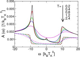
Figure 2: Temperature dependence of the spectral function for an exchange coupling of the impurity’s spins equal to ten times the Kondo temperature, $I=10\ {k_{B}}T_{K}^{0}$, for the Anderson model, Eq. (8a). The energy axis is expressed in $T_{K}^{0}$ units, such that the inelastic thresholds appear at $\pm 10$. As the temperature is raised (from 0.2 $T_{K}^{0}$ to 2.4 $T_{K}^{0}$), the Kondo-like peaks located close to the inelastic thresholds are smeared and finally even the inelastic gap disappears. Dashed lines are the results for the one-electron theory, that accounts for the inelastic changes of the spectral function where all impurities are assumed to initially be in their singlet state.

The comparison of the one-electron and many-body spectral functions shows that the apparent energy thresholds are displaced one with respect to the other. This is already apparent in Fig. 1 where the threshold coincides with the mid-point of the inelastic step for the one-electron spectral function but the mid-points of the inelastic steps in the many-body results are clearly shifted from the energy threshold. Figure 2 shows a common point where the one-electron spectral functions cross for the five considered temperatures. However, there is no common crossing point in the many-body curves and their behavior is controlled by the temperature evolution of the Kondo-like peaks.

For the SU(4) Kondo effect (case of a vanishing exchange interaction, $I$), the Kondo peak is greatly diminished at $T\approx T_{K}^{0}$. This is seen in Fig. 3 $(a)$, where the $I=0$, SU(4) Kondo peak is plotted for several temperatures. Figure 3 has been obtained by solving the $T$-matrix, $\mathcal{T}$, for the Coqblin-Schrieffer Hamiltonian, Eq. (11). The figure shows the imaginary part of the $T$-matrix times the density of states $\rho$ as a function of the electron energy $\omega$. This is equivalent to plotting the spectral function as a function of $\omega$, since the hybridization function $\Gamma$ is the proportionality factor connecting them. Comparison of Figs. 2 and 3 shows the equivalence of both Hamiltonians, Eqs. (8a) and (11), and of the solution methods.

Surprisingly, when the temperature behavior of the inelastic Kondo-like peaks is studied (Fig. 3 $(b)$), we observe that the peaks survive the temperature increase much longer than the SU(4) peaks (Fig. 3 $(a)$). Figure 3 $(b)$ shows $-Im\rho\mathcal{T}$ as in $(a)$, for $I=256\,k_{B}T_{K}^{0}$. However, we see that the spectral features are still important at $T\approx T_{K}^{0}$, and even at $T=50\;T_{K}^{0}$ spectral peaks are still visible. However, at $T=2.0\;T_{K}^{0}$ the SU(4) peaks are very diminished, Fig. 3$(a)$. This shows that the inelastic process with an excitation energy equal to $I$ sets in a new energy scale that controls the spectral variation with temperature. Only when $T_{K}^{0}$ is very small (results not shown here), we recover the one-electron limit. Hence, the conditions where many-body effects are not observable, while inelastic effects are observable are $k_{b}\;T_{K}^{0}\ll k_{b}\;T\ll I$.

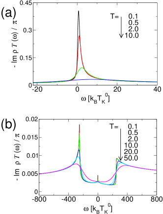
Figure 3: Imaginary part of the $T$-matrix times the density of states $\rho$ for different temperatures in $T_{K}^{0}$ units. $(a)$ SU(4) case for the spin 1/2 problem obtained when the exchange interaction between the two localized spins is set to zero, $I=0$. $(b)$ the singlet-triplet excitation for a large value of the exchange integral, $I=256\,k_{B}T_{K}^{0}$.

For temperatures above $I$, the two inelastic peaks coalesce giving rise to a a single broad peak, similarly to the SU(4) limit. This variation appears in more detail in Fig. 4 which presents the heights of the inelastic Kondo peaks relative to their value at low T as functions of the temperature.

For $I=0$, the peak heights are approximately described by the blue curve (Fig. 4) given by:

$$A_{max}=\frac{1}{1+(2^{1/s}-1)(T/T_{K}^{0})^{s}},$$ (15)

with $s=0.4$. The same expresion, for $s=0.21$ has been used to fit the results for the conductance in the Kondo regime from a renormalization group calculation Goldhaber-Gordon et al. (1998); Costi et al. (1994). Since, the fitted quantities ($T$-matrix vs conductance) and the system (SU(4) vs SU (2)) are not the same, it is not surprising that $s$ is different. This fit ensures that the peak has dropped to 1/2 at $T=T_{K}^{0}$, which shows that the expression for the Kondo temperature, $T_{K}^{0}$ given by Eq. (9) is a satisfactory approximation for both the NCA and SCLA.

Figure 4 also plots the temperature evolution of the heights of the two inelastic Kondo peaks for $I=10\,k_{B}T_{K}^{0}$ (down triangles and diamonds for lower and uppper peaks, resp.) and $I=256\,k_{B}T_{K}^{0}$ (squares and up triangles for lower and uppper peaks, resp.). Each peak height is normalized to its value for $T\approx 0$. At $T\approx 6\,T_{K}^{0}$, the two peaks of the $I=10\,k_{B}T_{K}^{0}$ case coalesce and form a single peak. In order to show this clearly in Fig. 4 we have to change the normalization of the peak heights above 6 $T_{K}^{0}$. We chose to normalize the single peak above 6 $T_{K}^{0}$ as the high energy peak. This increases the discontinuity in the down-triangle curve but preserves the diamond curve. Beyond $T\approx 10\,T_{K}^{0}$ the curve evolves more softly. This behavior shows that $I$ is the energy scale that governs the spectral-feature evolution at high temperatures. For the $I=256\,k_{B}T_{K}^{0}$ cases, the plotted temperature range (see e.g. in Fig. 3 $(b)$) does not reach a point at which the two peaks overlap significantly.

The different sensitivity to temperature increase in the inelastic case as compared to the ’usual’ Kondo problem, can be attributed to the different role of electron-hole pairs. Decoherence increases as a temperature rise induces more electron-hole pairs. For the usual Kondo case, a Fermi electron is scattered by the impurity, hence thermal electron-hole pairs are very efficient in causing the electron decoherence. However, in the inelastic case, an excited electron is scattered by the impurity and so it concerns the energy range around I. Hence, decoherence becomes particularly efficient when the thermal electron-hole pairs have enough energy to reach the inelastic transition range, i.e. when the temperature is of the order of the excitation energy. This explains why as we increase $I$, the Kondo-like peaks survive at higher temperatures.

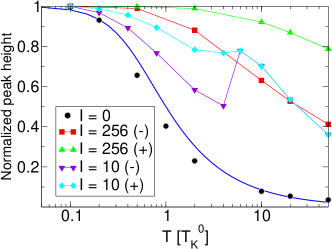
Figure 4: Maximum value of the spectral functions of Figs. 2 and 3 as a function of temperature normalized to the value at $T\approx 0$. Black dots: peak near the Fermi energy for $I=0$ (Fig. 3$(a)$); mauve down triangles: peak near $\omega=-10\,k_{B}T_{K}^{0}$ and cyan diamonds: peak near $\omega=-10\,k_{B}T_{K}^{0}$ for $I=10\,k_{B}T_{K}^{0}$ (Fig. 2); red squares: peak near $\omega=-256\,k_{B}T_{K}^{0}$ and green triangles: peak near $\omega=256\,k_{B}T_{K}^{0}$ for $I=256\,k_{B}T_{K}^{0}$ (Fig. 3$(b)$). The blue line is an empirical fit to the results for $I=0$ that displays at $T=T_{K}^{0}$ a maximum value half of that at $T=0$. The normalization of the down-triangle curve has been changed above $T=6\,T_{K}^{0}$, due to the coalescence of the two inelastic Kondo-like peaks at high $T$ (see text for details).

III.6 Orbital energy dependence of the excitation threhold

The inelastic spectra show Kondo-like features at the excitation thresholds. Zero-energy Kondo peaks are basically determined by the value of the Kondo temperature, $T_{K}^{0}$, and of the orbital energy, $\epsilon$. $T_{K}^{0}$ is responsible for the zero-temperature width of the Kondo peak and $\epsilon$ is an important factor for the actual shape of the Kondo peak by virtue of the Friedel-Langreth sum rule Langreth (1966); Hewson (1993). For this reason, we have studied the variation of the inelastic features with the orbital energy, keeping the Kondo temperature, $T_{K}^{0}$, constant.

Figure 5 shows the evolution of the inelastic features for five different values of the orbital energy (excitation energy $I$ equal to $4\,k_{B}T_{K}^{0}$ in Fig. 5(a) and to $32\,k_{B}T_{K}^{0}$ in Fig. 5(b)). The first four orbital-energy values increase by a factor of two: $|\epsilon|=110,\,220,\,440$  and $880\;k_{B}T_{K}^{0}$. The fifth value is computed using the Coqblin-Schrieffer Hamiltonian, Eq. (11), that corresponds to the Kondo-limit or $\epsilon\rightarrow-\infty$. The negative-energy peaks of the spectral functions have been normalized to one by multiplying the full spectral function by a constant number. The behavior of the low and high- energy tails can be understood just by the change in the density of states as the orbital energy shifts, because $T_{K}^{0}$ is kept constant and hence, the ratio $\epsilon/\Gamma$ is constant, where $2\pi\Gamma$ is the width of the one-electron peak originating at $\epsilon$. Hence, as $\epsilon$ approaches $-\infty$, the width $2\pi\Gamma$ increases. For $|\epsilon|=110\;k_{B}T_{K}^{0}$, the orbital resonance is close to the Fermi energy, and hence, the density of states drops rapidly, while for a larger value, the resonance is far from the Fermi energy and much broader, dropping more slowly following the trends of Fig. 5.

Despite the relation of the peaks at threshold with Kondo features, it is difficult to conclude on some type of extension of the Fermi-Langreth sum rule since the two peaks at the inelastic thresholds present different behaviors.

As $|\epsilon|$ increases the peaks at thresholds move away from the threshold energy towards positive energies. However, the inset shows that the $\epsilon\rightarrow-\infty$ case for $I=32\;k_{B}\,T_{K}^{0}$ is anomalous in the sense that it presents an extra broadening instead of a positive-energy shift. This hints at some saturation effect as the energy scales increase.

It is noteworthy that the evolution of the negative-energy peaks is faster than the positive ones. The peaks at negative energy are also narrower than the positive energy ones and their relative heights change depending on the values of $I$ and $\epsilon$. While for $I=4\;k_{B}T_{K}^{0}$ the positive-energy peak is equal or larger than the negative-energy case, for $I=32\;k_{B}T_{K}^{0}$ they are smaller.

Figure 5 also shows that the deviation of the peaks from the inelastic thresholds, $\Delta I$, depends on $I$. We study this behavior in the next section.

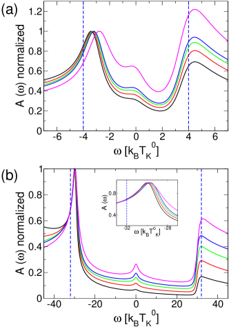
Figure 5: Normalized spectral function as a function of the electron energy in units of the Kondo temperature, $T_{K}^{0}$. Case (a) corresponds to an excitation energy $I=4\,k_{B}T_{K}^{0}$ as depicted by the vertical dashed line. Case (b) corresponds to the $I=32\,k_{B}T_{K}^{0}$ case. The curves correspond to orbital energies $|\epsilon|=110,220,440,800\,k_{B}T_{K}^{0}$ for the curves in increasing spectral function in the positive-energy part of the graphs. The topmost curve has been computed using the equivalent Coqblin-Schrieffer Hamiltonian, and hence corresponds to the $\epsilon\rightarrow-\infty$ case. The insets magnifies the negative-energy peaks of the $I=32\,k_{B}T_{K}^{0}$ case. The temperature is $T=0.1\,T_{K}^{0}$

III.7 Asymptotic behavior of the threshold renormalization

All the above results show that the apparent inelastic thresholds shift as $I$ increases. Actually, the threshold shifts lead to a reduction of the inelastic gap. We can quantify this reduction by studying the appeareance of singularities in the resolvents that translate into peaks of the spectral function. In order to perform this study, we have used the above SCLA applied to the Coqblin-Schrieffer model.

Let $E_{0}$ and $E_{1}$ be the bare energies of the spin zero and spin one multiplets. The dressed multiplet energies $E_{0}^{*},E_{1}^{*}$ are given by solving the equations

$$E_{0}^{*} =E_{0}+\Re\left\{\Sigma(E_{0}^{*})\right\}$$

$$E_{1}^{*} =E_{1}+\Re\left\{\Sigma(E_{1}^{*})\right\},$$

where $\Sigma(\omega)$ is the pseudo-fermion self-energy. Since $I$ is equal to the singlet-triplet excitation energy, $I=E_{1}-E_{0}$, the threshold shift $\Delta I$ is given by

$$\Delta I=(E_{1}^{*}-E_{0}^{*})-(E_{1}-E_{0})=\Re\left\{\Sigma(E_{1}^{*})-\Sigma(E_{0}^{*})\right\}$$ (16)

Figure 6: Shift of the excitation energy, $|\Delta I|$, versus excitation energy $I$, crosses. All results are in $T_{K}^{0}$ units. Full line, fit of the numerical results to the function $|\Delta I|=\sqrt{ax^{2}+bx+c}$ where $x=I/ln(I/k_{B}\,T_{K}^{0})$. Hence, for values of $I$ larger than the ones of the present graph, the threshold shift, $|\Delta I|$, follows the asymptotic behavior $\sim I/ln(I/k_{B}\,T_{K}^{0})$.

Figure 6 shows the absolute value of the threshold shift as a function of the excitation energy $I$ in $T_{K}^{0}$ units. The function $|\Delta I|=\sqrt{ax^{2}+bx+c}$ with $x=I/ln(I)$ is an excellent fit for a large range of values of $I$. The fitting parameters are $a=0.0029$, $b=0.6700$ and $c=-3.3361$. Hence, for asymptotically large excitation energies, $|\Delta I|$ is of the order of $\sqrt{a}\ I/ln(I/k_{B}\,T_{K}^{0})$. This result is completely equivalent to the asymptotic behavior found for the shift of Kondo peaks under a magnetic field $B$ as estimated by Rosch and co-workers Rosch et al. (2003) and by studying the shift of spinon density of states under a magnetic field by Moore and Wen Moore and Wen (2000).

IV Discussion and conclusions

The above results show that many-body effects in magnetic IETS can be readily studied with usual Kondo-physics tools such as the self-consistent approaches NCA (for the Anderson model) and SCLA (for the Coqblin-Schrieffer one). Comparison with one-electron approaches Lorente and Gauyacq (2009) is in overall agreement and permits us to discern many-body effects that appear as a consequence of the impurity excitation’s coherence when the inelastic channels open. Here, we have studied the case of a singlet-triplet excitation, when the tunneling electrons have enough energy to overcome the singlet-triplet energy difference, $I$. This situation has been achieved experimentally in carbon nanotubes Paaske et al. (2006). Related experiments are the ones performed in Mn dimers Hirjibehedin et al. (2006). However, we expect these results to be of relevance for many IETS cases when the energy scales correspond to the Kondo ones.

The one-electron magnetic IETS theory runs parallel to the NCA. Namely, a spin excitation takes place via a charge transfer process. During this process the magnetic impurity changes its charge state. The decay of the charge state back into the adsorbed state can lead to a final state different from the initial one. This is the essence of the excitation process. NCA builds on the same idea in a self-consistent way such that charge exchange processes are included to all orders, keeping their coherence. Hence, Kondo-like features are included.

The many-body features revealed in this study can be summarized by the distorsion of the spectral properties of the impurity as compared to the one-electron case. Two peaks appear close to the inelastic thresholds that are due to spin fluctuations when at least two spin states become degenerate similarly to the ’usual’ Kondo case. The inelatic peaks are shifted with respect to the energy degeneracy point (the inelastic threshold). This leads to a narrowing of the inelastic gap. This narrowing increases as $I$ increases following the asymptotic law $|\Delta I|\sim I/ln(I/k_{B}\ T_{K}^{0})$. This is exactly the behavior found for a Kondo peak split by a magnetic field Moore and Wen (2000).

The resemblance of the present results with those for the Kondo effect in the presence of magnetic fields Dickens and Logan (2001); Rosch et al. (2003); Moore and Wen (2000) is due to the similarities between the two physical processes: in both cases, there is a magnetic excitation, in the present case due to the interaction between two localized spins, and in the magnetic-field case due to Zeeman energy splitting, and when the electron energy is large enough to open the excited channel, the ground and excited states are connected via inelastic spin-flip electron collisions (note that in the present case involving singlet-triplet transitions, these are both of spin-flip and non-spin-flip type).

Finally, the many-body effects described here should be observable at large enough Kondo temperatures, $T_{K}^{0}$. This implies that the molecule should be in the Kondo regime ($|\epsilon|<\Gamma$) but with a sizable $T_{K}^{0}$ (i.e. $|\epsilon|/\Gamma\sim O(1)$ ). In this situation, peaks at the inelastic thresholds will be of many-body nature, leading to a strong renormalization of the thresholds (see Fig. 6) which can have important consequences in the use of magnetic IETS as a spectroscopic tool. The actual observation of many-body features may however depend on the measuring procedure. STM measurements involve several orbitals that may or may not be involved in Kondo physics. For realistic systems, the identification of spectral function with measured conductance is sometimes not straightforward. Although the Kondo peak may prevail in the spectral function, the multi-orbital character of the STM conductance can lead to channel interference and other effects with the consequent appearance of complex Fano profiles Madhavan et al. (2001); Újsághy et al. (2000).

Our results show that once Kondo-like features are present, they are more robust than usual Kondo peaks. Indeed, while Kondo peaks completely disappear at temperatures a few times the Kondo temperature, inelastic many-body features survive in this temperature range, if the temperature is smaller than the excitation energy. Actually, two energy scales determine the many-body properties of IETS: the coherence scale given by $k_{B}\ T_{K}^{0}$, and the excitation energy. Hence, not surprisingly as noticed by Hurley and coworkers Hurley et al. (2011), some experimental IETS show spike-like features at the IETS thresholds, where the results of our present work should be taken into consideration.

References

- Heinrich et al. (2004) A. J. Heinrich, J. A. Gupta, C. P. Lutz, and D. M. Eigler, Science 306, 466 (2004).
- Hirjibehedin et al. (2007) C. F. Hirjibehedin, C.-Y. Lin, A. F. Otte, M. Termes, C. P. Lutz, B. A. Jones, and A. J. Heinrich, Science 317, 1199 (2007).
- Hirjibehedin et al. (2006) C. F. Hirjibehedin, C. P. Lutz, and A. J. Heinrich, Science 312, 1021 (2006).
- Tsukahara et al. (2009) N. Tsukahara, K.-i. Noto, M. Ohara, S. Shiraki, N. Takagi, Y. Takata, J. Miyawaki, M. Taguchi, A. Chainani, S. Shin, et al., Phys. Rev. Lett. 102, 167203 (2009).
- Chen et al. (2008) X. Chen, Y.-S. Fu, S.-H. Ji, T. Zhang, P. Cheng, X.-C. Ma, X.-L. Zou, W.-H. Duan, J.-F. Jia, and Q.-K. Xue, Phys. Rev. Lett. 101, 197208 (2008).
- Fransson (2009) J. Fransson, Nano Letters 9, 2414 (2009).
- Fernández-Rossier (2009) J. Fernández-Rossier, Phys. Rev. Lett. 102, 256802 (2009).
- Persson (2009) M. Persson, Phys. Rev. Lett. 103, 050801 (2009).
- Lorente and Gauyacq (2009) N. Lorente and J.-P. Gauyacq, Phys. Rev. Lett. 103, 176601 (2009).
- Inoshita et al. (1993) T. Inoshita, A. Shimizu, Y. Kuramoto, and H. Sakaki, Phys. Rev. B 48, 14725 (1993).
- Inoshita et al. (1997) T. Inoshita, Y. Kuramoto, and H. Sakaki, Superlattices and Microstructures 22, 75 (1997), ISSN 0749-6036.
- Liang et al. (2002) W. Liang, M. Bockrath, and H. Park, Phys. Rev. Lett. 88, 126801 (2002).
- Nygard et al. (2000) J. Nygard, D. H. Cobden, and P. E. Lindelof, Nature (London) 408, 342 (2000).
- Kogan et al. (2003) A. Kogan, G. Granger, M. A. Kastner, D. Goldhaber-Gordon, and H. Shtrikman, Phys. Rev. B 67, 113309 (2003).
- Paaske et al. (2006) J. Paaske, A. Rosch, P. Wolfle, N. Mason, C. M. Marcus, and J. Nygard, Nat. Phys. 2, 460 (2006).
- Cornaglia et al. (2004) P. S. Cornaglia, H. Ness, and D. R. Grempel, Phys. Rev. Lett. 93, 147201 (2004).
- Paaske and Flensberg (2005) J. Paaske and K. Flensberg, Phys. Rev. Lett. 94, 176801 (2005).
- Parks et al. (2007) J. J. Parks, A. R. Champagne, G. R. Hutchison, S. Flores-Torres, H. D. Abruña, and D. C. Ralph, Phys. Rev. Lett. 99, 026601 (2007).
- Cornaglia et al. (2007) P. S. Cornaglia, G. Usaj, and C. A. Balseiro, Phys. Rev. B 76, 241403 (2007).
- Fernández-Torrente et al. (2008) I. Fernández-Torrente, K. J. Franke, and J. I. Pascual, Phys. Rev. Lett. 101, 217203 (2008).
- Zaránd et al. (2004) G. Zaránd, L. Borda, J. von Delft, and N. Andrei, Phys. Rev. Lett. 93, 107204 (2004).
- Borda et al. (2007) L. Borda, L. Fritz, N. Andrei, and G. Zaránd, Phys. Rev. B 75, 235112 (2007).
- Zitko and Pruschke (2010) R. Zitko and T. Pruschke, New Journal of Physics 12, 063040 (2010).
- Hurley et al. (2011) A. Hurley, N. Baadji, and S. Sanvito, Phys. Rev. B 84, 115435 (2011).
- Loth et al. (2010) S. Loth, K. von Bergmann, M. Termes, A. F. Otte, C. P. Lutz, and A. J. Heinrich, Nature Physics 6, 340 (2010).
- Delgado and Fernandez-Rossier (2010) F. Delgado and J. Fernandez-Rossier, Phys. Rev. B 82, 134414 (2010).
- Novaes et al. (2010) F. D. Novaes, N. Lorente, and J.-P. Gauyacq, Phys. Rev. B 82, 155401 (2010).
- Korytár and Lorente (2011) R. Korytár and N. Lorente, Journal of Physics: Condensed Matter 23, 355009 (2011).
- Bork et al. (2011) J. Bork, Y.-h. Zhang, L. Diekhöner, L. Borda, P. Simon, J. Kroha, P. Wahl, and K. Kern, Nature Physics 7, 901 (2011).
- Maekawa et al. (1985) S. Maekawa, S. Takahashi, S.-i. Kashiba, and M. Tachiki, Journal of the Physical Society of Japan 54, 1955 (1985).
- Gauyacq et al. (2010) J.-P. Gauyacq, F. D. Novaes, and N. Lorente, Phys. Rev. B 81, 165423 (2010).
- Roura Bas and Aligia (2009) P. Roura Bas and A. A. Aligia, Phys. Rev. B 80, 035308 (2009).
- Bas and Aligia (2010) P. R. Bas and A. A. Aligia, Journal of Physics: Condensed Matter 22, 025602 (2010).
- Cornaglia et al. (2011) P. S. Cornaglia, P. Roura Bas, A. A. Aligia, and C. A. Balseiro, European Physics Letters 93, 47005 (2011).
- Meir and Wingreen (1992) Y. Meir and N. S. Wingreen, Phys. Rev. Lett. 68, 2512 (1992).
- Ness (2006) H. Ness, Journal of Physics: Condensed Matter 18, 6307 (2006).
- Monturet and Lorente (2008) S. Monturet and N. Lorente, Phys. Rev. B 78, 035445 (2008).
- Lauhon and Ho (2001) L. Lauhon and W. Ho, Rev. Sci. Inst. 72, 216 (2001).
- Lambe and Jaklevic (1968) J. Lambe and R. Jaklevic, Phys. Rev. 165, 821 (1968).
- Schrieffer and Wolff (1966) J. R. Schrieffer and P. A. Wolff, Phys. Rev. 149, 491 (1966).
- Hewson (1993) A. C. Hewson, The Kondo Problem to Heavy Fermions, Cambridge studies in magnetism (Cambridge University Press, 1993).
- Coqblin and Schrieffer (1969) B. Coqblin and J. R. Schrieffer, Phys. Rev. 185, 847 (1969).
- Bickers (1987) N. Bickers, Reviews of Modern Physics 59, 845 (1987).
- Rosch et al. (2001) A. Rosch, J. Kroha, and P. Wölfle, Phys. Rev. Lett. 87, 156802 (2001).
- Hettler et al. (1998) M. H. Hettler, J. Kroha, and S. Hershfield, Phys. Rev. B 58, 5649 (1998).
- Tersoff and Hamann (1985) J. Tersoff and D. R. Hamann, Phys. Rev. B 31, 805 (1985).
- Lorente and Persson (2000) N. Lorente and M. Persson, Phys. Rev. Lett. 85, 2997 (2000).
- Kirchner and Kroha (2002) S. Kirchner and J. Kroha, Journal of Low Temperature Physics 126, 1233 (2002).
- Goldhaber-Gordon et al. (1998) D. Goldhaber-Gordon, J. Göres, M. A. Kastner, H. Shtrikman, D. Mahalu, and U. Meirav, Phys. Rev. Lett. 81, 5225 (1998).
- Costi et al. (1994) T. A. Costi, A. C. Hewson, and V. Zlatic, Journal of Physics: Condensed Matter 6, 2519 (1994).
- Langreth (1966) D. C. Langreth, Phys. Rev. 150, 516 (1966).
- Rosch et al. (2003) A. Rosch, T. A. Costi, J. Paaske, and P. Wölfle, Phys. Rev. B 68, 014430 (2003).
- Moore and Wen (2000) J. E. Moore and X.-G. Wen, Phys. Rev. Lett. 85, 1722 (2000).
- Dickens and Logan (2001) N. L. Dickens and D. E. Logan, Journal of Physics: Condensed Matter 13, 4505 (2001).
- Madhavan et al. (2001) V. Madhavan, W. Chen, T. Jamneala, M. F. Crommie, and N. S. Wingreen, Phys. Rev. B 64, 165412 (2001).
- Újsághy et al. (2000) O. Újsághy, J. Kroha, L. Szunyogh, and A. Zawadowski, Phys. Rev. Lett. 85, 2557 (2000).