Searching for the first stars with the Gaia mission

Abstract

Aims. We construct a theoretical model to predict the number of orphan afterglows (OA) from gamma-ray bursts (GRBs) triggered by primordial metal-free (Pop III) stars expected to be observed by the Gaia mission. In particular, we consider primordial metal-free stars that were affected by radiation from other stars (Pop III.2) as a possible target.

Methods. We use a semi-analytical approach that includes all relevant feedback effects to construct cosmic star formation history and its connection with the cumulative number of GRBs. The OA events are generated using the Monte Carlo method, and realistic simulations of Gaia’s scanning law are performed to derive the observation probability expectation.

Results. We show that Gaia can observe up to 2.28 $\pm$ 0.88 off-axis afterglows and 2.78 $\pm$ 1.41 on-axis during the five-year nominal mission. This implies that a nonnegligible percentage of afterglows that may be observed by Gaia ($\sim 10\%$) could have Pop III stars as progenitors.

1 Introduction

The first stars (hereafter, Pop III-primordial metal-free) in the Universe are thought to have played a crucial role in the early cosmic evolution by emitting the first light and producing the first heavy elements (Bromm et al. 2009). Understanding such objects is very important since their detection would permit the pristine regions of the Universe to be probed. However, there has been no direct observation of the so-called Pop III stars up to now.

Pop III stars may produce collapsar gamma-ray bursts (GRBs) whose total isotropic energy could be $\approx 2$ orders of magnitude larger than average (Barkov 2010; Komissarov & Barkov 2010; Mészáros & Rees 2010; Suwa & Ioka 2011; Toma et al. 2011). Even if the Pop III star has a supergiant hydrogen envelope, the GRB jet can break out of it because of the long-lasting accretion of the envelope itself (Nagakura et al. 2012; Suwa & Ioka 2011). It is of great importance to study the rate and detectability of Pop III GRB prompt emissions and afterglows in current and future surveys. We explore here the possibility to observe these objects through their afterglows (Toma et al. 2011). Observations of GRB afterglows make it possible to derive physical properties of the explosion mechanism and the circumburst medium. It is intriguing to search for signatures of metal-poor stars in the GRB afterglows at low and high redshifts.

GRB optical afterglows are one of the possible transients to be detected by the Gaia mission. Recently Japelj & Gomboc (2011) explored the detectability of such afterglows with Gaia using a Monte Carlo approach that inspired us. As the GRB jet sweeps the interstellar medium, the Lorentz factor of the jet is decelerated and the jet starts to expand sideways, eventually becoming detectable by off-axis observers. These afterglows are not associated with the prompt GRB emission and are called orphan afterglows (OA) (Nakar et al. 2002; Rossi et al. 2008).

De Souza et al. (2011) showed that, considering EXIST specifications, we can expect to observe a maximum of $\approx 0.08$ GRBs with $z>10$ per year originating from primordial metal-free stars (Pop III.1) and $\approx 20$ GRBs with $z>6$ per year coming from primordial metal-free stars that were affected by the radiation from other stars (Pop III.2). In the context of the current Swift satellite, $\approx 0.2$ GRBs with $z>6$ per year from Pop III.2 stars are expected. These numbers reflect the fact that, compared to Pop III.1 stars, Pop III.2 stars are more abundant and can be observed in a lower redshift range, which makes them more suitable targets. In the light of such results, the calculations presented here will focus on Pop III.2 stars alone.

Searches have been made of OAs by both X-ray surveys (Grindlay 1999; Greiner et al. 2000) and optical searches (Becker et al. 2004; Rykoff et al. 2005; Rau et al. 2006; Malacrino et al. 2007). The purpose of the present paper is to calculate the Pop III.2 GRB OA rate that might be detected by the Gaia mission (for more details about Gaia, see, e.g., Perryman et al. 2001; Lindegren 2009).

The Gaia mission is one of the most ambitious projects of modern astronomy. It aims to create a very precise tridimensional, dynamical, and chemical census of our Galaxy from astrometric, spectrophotometric, and spectroscopic data. In order to do this, the Gaia satellite will perform observations of the entire sky in a continuous scanning created from the coupling of rotations and precession movements called the scanning law. For point sources, these observations will be unbiased and the data of all the objects bellow a certain limiting magnitude (G=20) will be transferred to the ground. Certainly, galactic and extragalactic sources will be among those objects.

Typically, Pop III.2 stars are formed in an initially ionized gas (Johnson & Bromm 2006; Yoshida et al. 2007). They are thought to be less massive than Pop III.1 stars but still massive enough to produce GRBs. Recent results from Greif et al. (2011) show that, instead of forming a single object, the gas in mini-halos fragments vigorously into a number of protostars with a range of different masses. It is not clear up to now how this initial range of mass will be mapped into the final mass function of Pop III stars. The most likely conclusion is that Pop III stars are less likely to reach masses in excess of $\sim 140M_{\odot}$, which consequently affect the estimated number of GRBs from Pop III.1. Hosokawa et al. (2011), performing state-of-the-art radiation-hydrodynamics simulations, showed that the typical mass of Pop III stars could be $\sim 43M_{\odot}$. Here we assume that this will not affect significantly the mass range assumed for Pop III.2 ($\sim 10-100M_{\odot}$).

The paper is organized as follows. In Sect. 2, we calculate the formation rate of primordial GRBs. In Sect. 3, we calculate the OA light curves and their redshift distribution. In Sect. 4, we discuss the details of the Gaia mission and derive the probability of a given event to be observed by Gaia. In Sect. 5, we discuss the results, and finally, in Sect. 6, we give our concluding remarks. Throughout the paper, we adopt the standard $\Lambda$ cold dark matter model with the best-fit cosmological parameters from Jarosik et al. (2011) (WMAP-Yr7), $\Omega_{\rm m}=0.267,\Omega_{\Lambda}=0.734$, and $H_{0}=71{\rm km}\leavevmode\nobreak\ {\rm s}^{-1}{\rm Mpc}^{-1}$.

2 GRB redshift distribution

To estimate the formation rate of GRBs from Pop III stars at a given redshift, we closely follow de Souza et al. (2011). Since long GRBs are expected to follow the death of very massive stars, their rate could provide a useful probe for cosmic star formation history (SFH) (e.g., Totani 1997; Ciardi & Loeb 2000; Bromm & Loeb 2002; Conselice et al. 2005; Campisi et al. 2010, 2011a; Ishida et al. 2011; de Souza et al. 2011; Robertson & Ellis 2012). However, the connection between the star formation rate (SFR) density and GRB rate is not clearly understood and can be redshift dependent (e.g., Yüksel et al. 2008; Kistler et al. 2009; Robertson & Ellis 2012). Since host galaxies of long-duration GRBs are often observed to be metal poor. Several studies connect the origin of long GRBs with the metallicity of their progenitors (e.g., Mészáros 2006; Woosley & Bloom 2006; Salvaterra & Chincarini 2007; Salvaterra et al. 2009; Campisi et al. 2011b). Consequently, the GRB-SFR connection could be dependent on the cosmic metallicity evolution. However, this connection is not yet completely understood, since there is also evidence of regions within GRB host galaxies known to possess higher metallicities (Levesque et al. 2010).

Despite such uncertainties, we expect the connection between SFR and GRBs to be less affected by this effect because Pop III stars and their environment are metal poor. In other words, Pop III stars are more likely to produce GRBs than ordinary stars. It is important to keep in mind that any prediction will be convolved with systematic effects that we are not taking into account. However, as pointed out in Ishida et al. (2011), the assumption is good enough to agree with available observational data.

We implicitly assume that the formation rate of long GRBs (duration longer than 2 sec) follows closely the SFH. The number of GRBs per comoving volume per time can be expressed as

$$\Psi_{\rm GRB}(z)=\eta_{\rm GRB}\Psi_{*}(z),$$ (1)

where $\eta_{\rm GRB}$ is the GRB formation efficiency and $\Psi_{*}$ is the SFR. Over a particular time interval, $\Delta t_{\rm obs}$, in the observer rest frame, the number of GRBs originating between redshifts $z$ and $z+dz$ is

$$\frac{{\rm d}N_{\rm GRB}}{{\rm d}z}=\Psi_{\rm GRB}(z)\frac{\Delta t_{\rm obs}}{1+z}\frac{{\rm d}V}{{\rm d}z},$$ (2)

where ${\rm d}V/{\rm d}z$ is the comoving volume element per redshift unit.

2.1 Star Formation History

To estimate the SFR at early epochs, we assume that stars are formed in collapsed dark matter halos (for more details, please see de Souza et al. 2011). The number of collapsed objects is given by the halo mass function (Hernquist & Springel 2003; Greif & Bromm 2006; Trenti & Stiavelli 2009). In what follows, we adopt the Sheth-Tormen function, $f_{\rm ST}$ (Sheth & Tormen 1999). To estimate the fraction of mass inside each halo capable of collapsing and forming stars, we include the following important feedback mechanisms:

1. $\rm H_{2}$ Photodissociation

   Hydrogen molecules (H₂) are the primary coolant in the gas within small-mass “mini-halos.” H₂ are also sensitive to ultra-violet radiation in the Lyman-Werner (LW) bands and can easily be suppressed by it. We model the dissociation effect by setting the minimum mass for halos that are able to host Pop III stars (Yoshida et al. 2003).

2. Reionization

   Inside growing Hii regions, the gas is highly ionized and the temperature is $\sim 10^{4}$ K. The volume-filling factor of ionized regions, $Q_{\rm{H\sc{II}}}(z)$, determines when the formation of Pop III.1 stars is terminated and switches to Pop III.2. To calculate $Q_{\rm{H\sc{II}}}(z)$, we closely follow Wyithe & Loeb (2003) as in de Souza et al. (2011).

3. Metal Enrichment

   Metal enrichment in the intergalactic medium (IGM) determines when the formation of primordial stars is terminated (locally) and switches from the Pop III mode to a more conventional mode of star formation. We assume that star-forming halos launch a wind of metal-enriched gas at $z\gtrsim 20$. Then we follow the metal-enriched wind propagation outward from a central galaxy with a given velocity $v_{wind}$, traveling over a comoving distance $R_{wind}$. We estimate the ratio of gas mass enriched by the wind to the total gas mass in each halo, and then we evaluate the average metallicity over cosmic scales as a function of redshift. We effectively assume that the so-called critical metallicity is very low (Schneider et al. 2002, 2003; Bromm & Loeb 2003; Omukai et al. 2005; Frebel et al. 2007; Belczynski et al. 2010). Therefore, Pop III stars are not formed in a metal-enriched region, regardless of the actual metallicity.

Rollinde et al. (2009) investigated the role of Pop III stars in the cosmic metallicity evolution, in particular, the local metallicity function of the Galactic halo. They show that Pop III SFR should not be larger than $3\times 10^{-3}M_{\odot}yr^{-1}Mpc^{-3}$ at any redshift. We also include this additional constraint as an upper limit for our optimistic model.

The top panel of Fig. 1 shows the upper limit for Pop III.2 SFR, based on de Souza et al. (2011) with the additional constraints cited above. The Pop III.2 SFR is compared with a compilation of independent measures from Hopkins & Beacom (2006) up to $z\approx 6$ and from observations of color-selected Lyman Break Galaxies (Mannucci et al. 2007; Bouwens et al. 2008, 2011), UV+IR measurements (Reddy et al. 2008), and GRB observations (Chary et al. 2007; Yüksel et al. 2008; Wang & Dai 2009) at higher $z$ (in the figure, these will be refereed to as H2006, M2007, B2008, B2011, R2008, C2007, Y2008, and W2009, respectively).

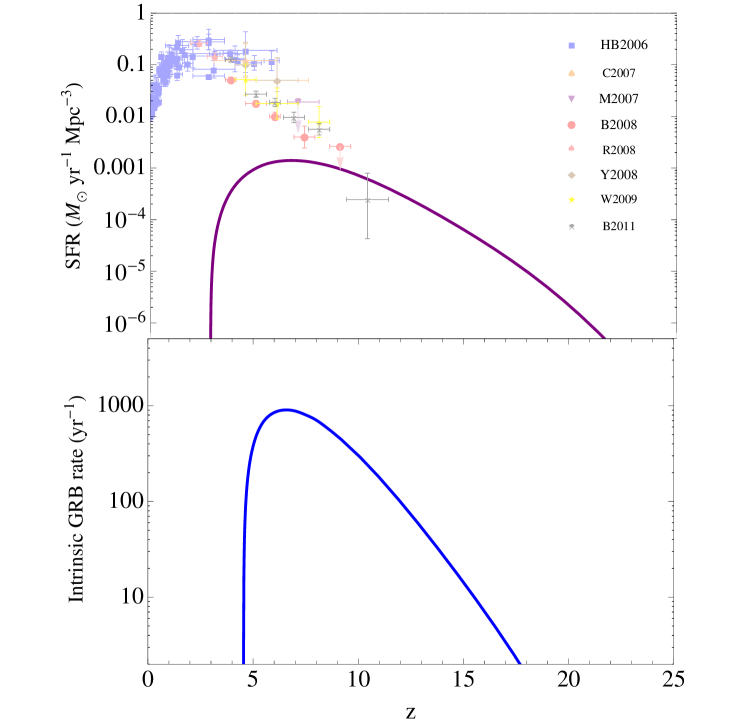
Figure 1: Top: optimistic model for Pop III.2 star formation rate (SFR) assuming a high star formation efficiency and low chemical enrichment. The light points are independent SFR determinations compiled from the literature.

Bottom: intrinsic GRB rate ${\rm d}N_{\rm GRB}/{\rm d}z$, i.e., the number of GRBs per year on the sky (on-axis + off-axis) according to Eq. (2). This represents our optimistic model assuming a high star formation efficiency for Pop III.2, slow chemical enrichment, GRB formation efficiency of $f_{GRB}=0.001$ and a Salpeter IMF.

2.2 Initial Mass Function and GRB Formation Efficiency

The stellar initial mass function (IMF) is critically important to determine the Pop III GRB rate. The IMF determines the fraction of stars with minimum mass that are able to trigger GRBs, $\sim 25M_{\odot}$ (Bromm & Loeb 2006). The $f_{\rm GRB}$ factor gives the fraction of stars in this range of mass that will produce GRBs.

The GRB formation efficiency factor per stellar mass is

$$\eta_{\rm GRB}=f_{\rm GRB}\frac{\int_{M_{\rm GRB}}^{M_{\rm up}}\phi(m)dm}{\int_{M_{\rm low}}^{M_{\rm up}}m\phi(m)dm},$$ (3)

where $\phi(m)$ is the stellar IMF for which we considered a power law with the standard Salpeter slope $\phi(m)\propto m^{-2.35},$ $M_{\rm low}$ and $M_{\rm up}$ are the minimum and maximum mass for a given stellar type (respectively $10M_{\odot}$ and $\sim 100M_{\odot}$ for Pop III.2), and $M_{\rm GRB}$ is the minimum mass able to trigger GRBs, which we set to be $25M_{\odot}$ (Bromm & Loeb 2006).

De Souza et al. (2011) placed upper limits on the intrinsic GRB rate (including the off-axis GRB). In the following, we set $f_{GRB}=0.001$ and $\eta_{\rm GRB}/f_{\rm GRB}\sim 1/87M_{\odot}^{-1}$ as an optimistic case, consistent with their results. The bottom panel of Fig. 1 shows the optimistic case for intrinsic GRB rate adopted in this work.

3 Number of Observed Orphans

3.1 Afterglow Model

To calculate the afterglow light curves of Pop III GRBs, we follow the standard prescription from Sari et al. (1998, 1999) and Mészáros (2006). The spectrum consists of power-law segments linked by critical break frequencies. These are $\nu_{\rm a}$ (the self-absorption frequency), $\nu_{\rm m}$ (the peak of injection frequency), and $\nu_{\rm c}$ (the cooling frequency), given by

$$\nu_{\rm m} \propto \leavevmode\nobreak\ (1+z)^{1/2}g(p)^{2}\epsilon_{e}^{2}\epsilon_{B}^{1/2}E_{\rm iso}^{1/2}t_{d}^{-3/2},$$

$$\nu_{\rm c} \propto \leavevmode\nobreak\ (1+z)^{-1/2}\epsilon_{B}^{-3/2}n^{-1}E_{\rm iso}^{-1/2}t_{d}^{-1/2},$$

$$\nu_{\rm a} \propto \leavevmode\nobreak\ (1+z)^{-1}\epsilon_{e}^{-1}\epsilon_{B}^{1/5}n^{3/5}E_{\rm iso}^{1/5},$$

$$F_{\nu,{\rm max}} \propto \leavevmode\nobreak\ (1+z)\epsilon_{B}^{1/2}n^{1/2}E_{\rm iso}d_{L}^{-2},\leavevmode\nobreak\$$ (4)

where $g(p)=(p-2)/(p-1)$ is a function of the energy spectrum index of electrons $(N(\gamma_{e})d\gamma_{e}\propto\gamma_{e}^{-p}d\gamma_{e}$, where $\gamma_{e}$ is the electron Lorentz factor), $\epsilon_{e}$ and $\epsilon_{B}$ are the efficiency factors (Mészáros 2006), $E_{iso}$ is the isotropic kinetic energy, n is the density of the medium, and $F_{\nu,{\rm max}}$ is the observed peak flux at luminosity distance $d_{L}$ from the source.

There are two types of spectra. If $\nu_{\rm m}<\nu_{\rm c}$, we call it the slow cooling case. The flux at the observer, $F_{\nu}$, is given by

$$F_{\nu}=\left\{\begin{array}[]{ll}(\nu_{\rm a}/\nu_{\rm m})^{1/3}(\nu/\nu_{\rm a})^{2}F_{\nu,{\rm max}},&\nu_{\rm a}>\nu,\\ (\nu/\nu_{\rm m})^{1/3}F_{\nu,{\rm max}},&\nu_{\rm m}>\nu>\nu_{\rm a},\\ (\nu/\nu_{\rm m})^{-(p-1)/2}F_{\nu,{\rm max}},&\nu_{\rm c}>\nu>\nu_{\rm m},\\ (\nu_{\rm c}/\nu_{\rm m})^{-(p-1)/2}(\nu/\nu_{\rm c})^{-p/2}F_{\nu,{\rm max}},&\nu>\nu_{\rm c}.\end{array}\right.$$ (5)

For $\nu_{\rm m}>\nu_{\rm c}$, called the fast cooling case, the spectrum is

$$F_{\nu}=\left\{\begin{array}[]{ll}(\nu_{\rm a}/\nu_{\rm c})^{1/3}(\nu/\nu_{\rm a})^{2}F_{\nu,{\rm max}},&\nu_{\rm a}>\nu,\\ (\nu/\nu_{\rm c})^{1/3}F_{\nu,{\rm max}},&\nu_{\rm c}>\nu>\nu_{\rm a},\\ (\nu/\nu_{\rm c})^{-1/2}F_{\nu,{\rm max}},&\nu_{\rm m}>\nu>\nu_{\rm c},\\ (\nu_{\rm m}/\nu_{\rm c})^{-1/2}(\nu/\nu_{\rm m})^{-p/2}F_{\nu,{\rm max}},&\nu>\nu_{\rm m}.\end{array}\right.$$ (6)

Initially the jet propagates as if it were spherical with an equivalent isotropic energy of $E_{\rm true}=\theta_{j}^{2}E_{\rm iso}/2$, where $\theta_{j}$ is the half-opening angle of the jet. Even if the prompt emission is highly collimated, the Lorentz factor drops $\gamma_{\rm d}<\theta_{j}^{-1}$ around the time

$$t_{\theta}\sim 2.14\left(\frac{E_{\rm iso}}{5\times 10^{54}}\right)^{1/3}\left(\frac{\theta_{j}}{0.1}\right)^{8/3}n^{-1/3}(1+z)\leavevmode\nobreak\ \rm days,$$ (7)

and the jet starts to expand sideways (Ioka & Mészáros 2005). Consequently, the jet becomes detectable by the off-axis observers. These afterglows are not associated with the prompt GRB emission.

Due to relativistic beaming, an observer located at $\theta_{obs}$, outside the initial opening angle of the jet ($\theta_{obs}>\theta_{j}$), will observe the afterglow emission only at $t\sim t_{\theta}$, when $\gamma_{\rm d}=\theta_{j}^{-1}$.

The received afterglow flux by an off-axis observer in the point source approximation, valid for $\theta_{obs}\gg\theta_{j}$, is related to that seen by an on-axis observer by (Granot et al. 2002; Totani & Panaitescu 2002; Japelj & Gomboc 2011)

$$F_{\nu}(\theta_{obs},t)=\xi^{3}F_{\nu/\xi}(0,\xi t),$$ (8)

where

$$\xi\equiv(1-\beta)/(1-\beta\cos\theta_{obs}),$$ (9)

and $\beta=\sqrt{1-1/\gamma_{\rm d}^{2}}$. The time evolution of the Lorentz factor in given by

$$\gamma_{\rm d}(t)=\left\{\begin{array}[]{ll}\theta_{\rm j}^{-1}\left(\frac{t}{t_{\rm j}}\right)^{-3/8}&t<t_{\rm j}\\ \theta_{\rm j}^{-1}\left(\frac{t}{t_{\rm j}}\right)^{-1/2}&t>t_{\rm j},\\ \end{array}\right.$$ (10)

where $t_{j}$ is the jet break time, $\approx 0.7(1+z)(E_{51}/n)^{1/3}(\theta_{j}/0.1)^{2}$ days (Sari et al. 1999). Figure 2 shows four examples of afterglows as a function of observed angle $\theta_{obs}$ for the case of $\theta_{j}=0.1$ at $z=3$ for typical parameters described in the figure. The flux is calculated for an observational frequency $\nu=5\times 10^{14}\rm{Hz}$ within the Gaia bandwidth. Depending on the parameters of the afterglow, the light curve can appear above the Gaia observational limits. Due to the large quantity of free parameters, a Monte Carlo approach is essential to explore the detectability of a large number of events and will be explained in the next section.

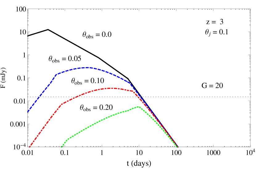
Figure 2: Example of afterglow light curve at $z=3$ as a function of observed angle, $\theta_{obs}$. We show the evolution of afterglow flux $F(mJy)$ as a function of time $t$ (days) and observed angle $\theta_{obs}$ for typical parameters: isotropic kinetic energy $E_{iso}=10^{54}$ erg, electron spectral index $p=2.5$, plasma parameters $\epsilon_{e}=0.1$, $\epsilon_{B}=0.01$, half-opening angle jet $\theta_{j}=0.1$, interstellar medium density $n=1cm^{-3}$ and frequency $\nu=5\times 10^{14}\rm{Hz}$. The horizontal dotted line is the integrated Gaia flux limit; solid black line, $\theta_{obs}=0$; dashed blue line, $\theta_{obs}=0.05$; dot-dashed red line, $\theta_{obs}=0.1$; dotted green line, $\theta_{obs}=0.20$.

3.2 Dust Extinction

A fraction of GRBs with X-ray or radio afterglows can be hidden by dust absorption from their host galaxies. The observed flux after extinction correction can be simply written as (see, e.g, Elíasdóttir et al. 2009)

$$F_{\nu}^{dust}=F_{\nu}(\theta_{obs},t)10^{-0.4A_{\lambda}},$$ (11)

where $A_{\lambda}$ is the extragalactic extinction along the line of sight, $A_{\lambda;ext}$, as a function of the wavelength $\lambda$ plus the extinction from the Milk Way, $A_{\lambda;MW}$.

For $A_{\lambda;ext}$, we adopted a simple Small Magellanic Cloud (SMC) type extinction model. The SMC model was already shown to provide good fits for several GRB afterglows observations (see, e.g, Elíasdóttir et al. 2009). For $A_{\lambda;MW}$, we use the average value 0.15 from observations of Schady et al. (2012) and adopt a typical value of 0.3 for $A_{V}$. In Fig. 3, we show the SMC extinction curve in comparison with other popular models, Large Magellanic Cloud (LMC) and Milky Way (MW). The model choice has no significant effect on our results, since all of them have a similar trend in the G band range. In Fig. 4, we show the effect of dust extinction in the spectral energy distribution (SED) of GRBs. The effect is significant in the G band ($\sim 5\times 10^{14}$ Hz), which will considerably decrease the detection rate of optical GRBs, mainly at high-z.

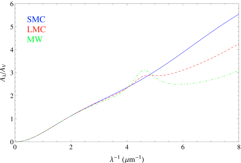
Figure 3: Extinction laws usually adopted in literature: the Small Magellanic Cloud (SMC) law (blue line), the Large Magellanic Cloud (LMC) law (red dashed line) and the Milky Way (MW) law (green dot-dashed line).

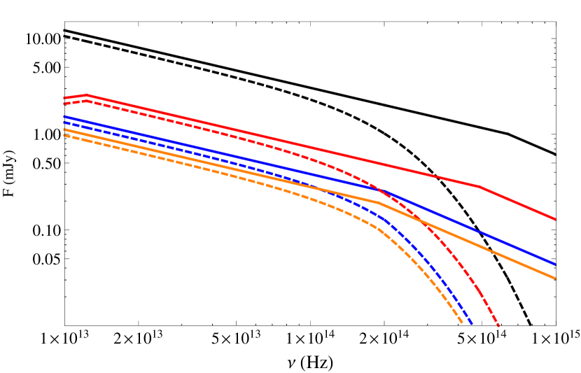
Figure 4: Example of a spectral energy distribution for observed GRBs with (dashed lines) and without (solid lines) extinction, assuming the SMC extinction law. We show the afterglow flux $F(mJy)$ as a function of frequency $\nu$ (Hz) for typical parameters: isotropic kinetic energy $E_{iso}=10^{54}$ erg, electron spectral index $p=2.5$, plasma parameters $\epsilon_{e}=0.1$, $\epsilon_{B}=0.01$, half-opening angle jet $\theta_{j}=0.1$, and interstellar medium density $n=1cm^{-3}$. The black line represents $\theta_{obs}=0$, t = 0.5 days, blue line, $\theta_{obs}=0$, t = 5 days, red line, $\theta_{obs}=0.05$, t = 0.5 days, and orange line, $\theta_{obs}=0.05$, t = 5 days.

3.3 IGM and DLA absorption

For high-z GRBs, much of the optical and near-infrared light will be absorbed by the $Ly\alpha$ forest, which provides a powerful tool to probe the reionization era (Miralda-Escude 1998; Mesinger & Furlanetto 2008; Ciardi et al. 2011). The GRB 050904 at z = 6.3 was the first attempt to probe the IGM through GRBs at the epoch of reionization by using the damping wing at wavelengths redward of the Lyman break (Totani et al. 2006; Kawai et al. 2006). The absorption by the neutral IGM can be approximated by (McQuinn et al. 2008)

$$\tau_{IGM}\approx 900\leavevmode\nobreak\ kms^{-1}\leavevmode\nobreak\ x_{\rm HI}\left(\frac{1+z_{host}}{8}\right)^{3/2}\times$$ (12)

$$\left(\frac{H(z_{host})R_{b}}{(1+z_{host})}-c\frac{\nu_{z}-\nu_{\alpha}}{\nu_{\alpha}}\right)^{-1},$$

where $\nu_{\alpha}$ is the rest frame of the $\rm Ly{\alpha}$ line, $R_{b}$ represents the size of an HII region surrounded by an IGM with neutral fraction $x_{\rm HI}$, $z_{host}$ is the redshift of the GRB host galaxy, and H(z) is the Hubble parameter for a $\Lambda$CDM cosmology. To estimate $x_{\rm HI}$, we use the prescription detailed in de Souza et al. (2011) (see Fig.1). The optical depth of the damped Ly$\alpha$ absorber (DLA), $\tau_{DLA}=N_{\rm HI}\sigma_{\alpha}[\nu_{obs}(1+z_{host})]$, can be computed by

$$\tau_{DLA}=7.26\left(\frac{N_{\rm HI}}{{10^{21}cm^{-2}}}\right)\left(\frac{1+z_{obs}}{8}\right)^{4}\times$$ (13)

$$\left(\frac{1+z_{host}}{8}\right)^{-2}\left(\frac{\Delta\lambda}{20\rm\AA\ }\right)^{-2},$$

(e.g., Barkana & Loeb 2004) where $\nu_{obs}=c/\lambda_{obs}$, $(1+z_{obs})=\lambda_{obs}/\lambda_{\alpha}$, $N_{\rm HI}$ is the total column density of $\rm HI$ in the host galaxy, and $\lambda_{obs}=\Delta\lambda+\lambda_{\alpha}(1+z)$. $N_{\rm HI}$ is randomly chosen assuming a cumulative distribution function scaling as $N_{\rm HI}^{0.3}$, between $10^{18}$ and $10^{21.5}cm^{-2}$ (see Chen et al. 2007; McQuinn et al. 2008). For each event, $R_{b}$ is chosen from a lognormal distribution between 1-100 Mpc motivated by a visual inspection in Fig. 5 from McQuinn et al. (2008).

3.4 Mock sample

The mock sample is generated by the Monte Carlo method assuming different probability distribution functions (PDF) for each quantity as explained below. The medium density $n$ is randomly chosen from a flat distribution within $0.1-1cm^{-3}$.

3.4.1 Redshift PDF

We generate the GRB events randomly in redshift with a PDF given by Eq. (2). The probability of a given GRB appearing at redshift $z$ is

$$P_{z}(z)=\frac{dN_{GRB}/dz}{\int_{0}^{z}(dN_{GRB}/dz)dz}.$$ (14)

The PDF was generated by $10^{5}$ random realizations based on Eqs. (2) and (14). Figure 5 shows the probability of finding a GRB at a given redshift, indicating that a 50% probability of having a GRB from a Pop III star is obtained in the redshift range $z\sim 7-11$ and a 95% probability in the range $z\sim 4-15$. Due to absorption from dust, IGM and DLA, the GRBs available for observation by Gaia are restricted to the range $z\sim 3-7$. This results in approximately $10^{4}$ GRBs during the entire Gaia nominal mission, which is the value adopted in this work.

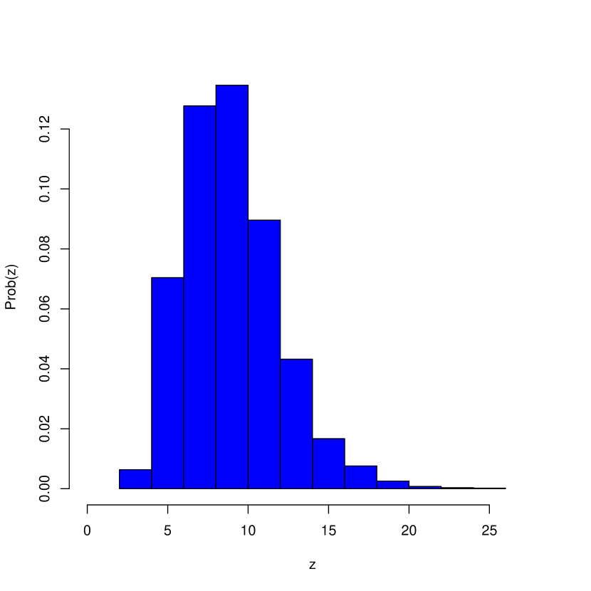
Figure 5: Redshift PDF. Probability of a given event appearing in a certain range of redshift.

3.4.2 Half-opening angle PDF

Using an empirical opening angle estimator, Yonetoku et al. (2005) derived the opening angle PDF of GRBs. Their PDF can be fitted by a power-lay   $\theta^{-2}$. Their results seem also compatible with the universal structured jet model (Perna et al. 2003). The jet opening angle usually ranges between $1^{\circ}-10^{\circ}$ (Frail et al. 2001; Cenko et al. 2009). For simplicity, we assume a similar power law in the range $\theta_{j}^{min}=0.01$ and $\theta_{j}^{max}=0.2$ to determine the PDF of $\theta_{j}$,

$$P_{\theta_{j}(\theta)}\propto\theta^{-2}.$$ (15)

Figure 6 shows the PDF of $\theta_{j}$ generated by $10^{5}$ realizations based on Eq. (15). The realizations were performed within the range $\theta_{j}=0.01-0.2$. The observational angle $\theta_{obs}$ was randomly chosen between $0-\pi$. From the relation $E_{\rm true}=\theta_{j}^{2}E_{\rm iso}/2$, we assume two fixed values for $E_{true}=(2.5-5)\times 10^{50}$ ergs, which imposes the limits $E_{iso}<5\times 10^{54}-10^{55}ergs$ respectively.

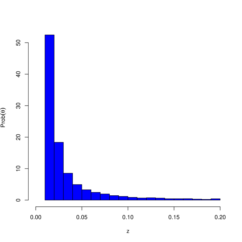
Figure 6: Half-opening angle jet PDF. Probability of a given GRB to have a particular $\theta_{j}$.

4 The Gaia mission

The Gaia satellite will perform observations of the entire sky, using a continuous scanning formed by the coupling of rotation and precession movements, the scanning law. This law guarantees that each point in the sky will be observed several times during the mission, as it can be seen in Fig. 7.

Similar to what happens with CCD meridian circles, in the referential of the satellite’s focal plane, the sky continuously moves from one side to the other while the satellite spins. During this time, the CCD charges are synchronously transferred to compensate for the sky’s apparent motion and allow the integration.

This continuous observation strategy requires an equally continuous reading of the CCDs. Also, since Gaia’s focal plane comprises 106 individual detectors, it is not possible to transfer the entire content of the focal plane to the Earth due to bandwidth limits. So, a continuous analysis of the focal plane observations is also performed on-board, aimed at the detection of astronomical sources. When a source is detected, a rectangular “window” comprising a few arcseconds around the detected source is created (its exact size and pixel binning depend on the focal plane’s CCD column). These windows are then transferred to the Earth.

For point sources, these observations will be unbiased and the data from all objects in the sky, bellow a certain limiting magnitude, will be sent to the ground. Certainly, among all those objects, not only galactic sources will be present, but also extragalactic ones. In particular, it is expected that point sources up to magnitude 20, in the Gaia passband G, will be “windowed” and transferred.

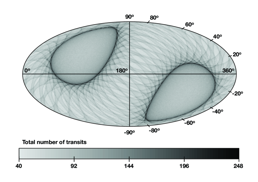
Figure 7: Number of times each region of the sky (in galactic coordinates) will be observed by the Gaia satellite during the entire mission.

As seen in Fig. 2, some of the OA events are expected to remain above this limiting magnitude for a certain amount of time. The question that remains is whether their duration (at G$\leqslant$20) is enough for them to be observed at a reasonable rate. Only two quantities play an important role in estimating the probability of Gaia observing single event from a Pop III.2: the time whichen the OA remains brighter than G=20, $\Delta t$, and the coordinates $(l_{gal},b_{gal})$ where the event takes place in the sky. Since those quantities are continuous distributions, it is necessary to analyze how the observation probability depends on them by building $P(\Delta t,l_{gal},b_{gal})$. In the present work, we proceed as follows.

For a given coordinate in the sky, we start by computing the inverse Gaia scanning law to derive a transit time list comprising the instants when Gaia’s telescopes will be pointing at that coordinate. To be as realistic as possible, we adopt the Gaia Data Processing and Analysis Consortium’s nominal implementation of it. Then, we randomly select a point in time during the entire mission lifetime in order to place an event of a certain duration $\Delta t$. Using the transit time list, we check if that event was observed, considering a time window of 4.4 seconds around each transit; this is the time needed for the signal to cross the detection CCD and enter the confirmation CCD. If there is a superposition between the event duration and this time window, the event is considered detected. This procedure is then repeated until the estimation of the detection probability, which is derived by simply dividing the number of detected events by the total, does not vary more than 1% between iterations. Finally, the whole procedure is repeated for each event duration $\Delta t$. As a consequence, we obtain an adequate time-sampling of the $P(\Delta t,l_{gal},b_{gal})$ distribution.

For the determination of the number of OA events observed by Gaia on the entire sky, the coordinate dependency can be averaged out, allowing $P(\Delta t,l_{gal},b_{gal})\sim P(\Delta t)\pm\epsilon$. This is possible because the scanning law is mostly known, so we can reasonably assume that the OA events take place randomly in the sphere.

The procedure described above was repeated for several positions on the sphere, and the mean and the standard deviation at each event duration were computed. To allow a good spatial sampling for the estimation of $P(\Delta t)\pm\epsilon$, we tessellate the celestial sphere at the hierarchical triangular mesh, level 4 (Kunszt et al. 2001). This means that the simulations were performed at the center of 2048 triangles of approximately equal areas.

Finally, to obtain the probabilities for the whole sky, an additional effect must be taken into account: the structure of our own Galaxy. Since the OAs are extragalactic events, the probability of observation at the galactic plane or bulge should be null or very small, due to extinction and crowding. In this work, we conservatively assumed a null value for the probability of OAs being observed at such regions of the sky (defined here as $|b|\leq 15^{\circ}$ for $345^{\circ}\leq l\leq 15^{\circ}$ and $|b|\leq 5^{\circ}$ otherwise).

The final results, representing the behavior of $P(\Delta t)\pm\epsilon$ can be seen in Fig. 8.

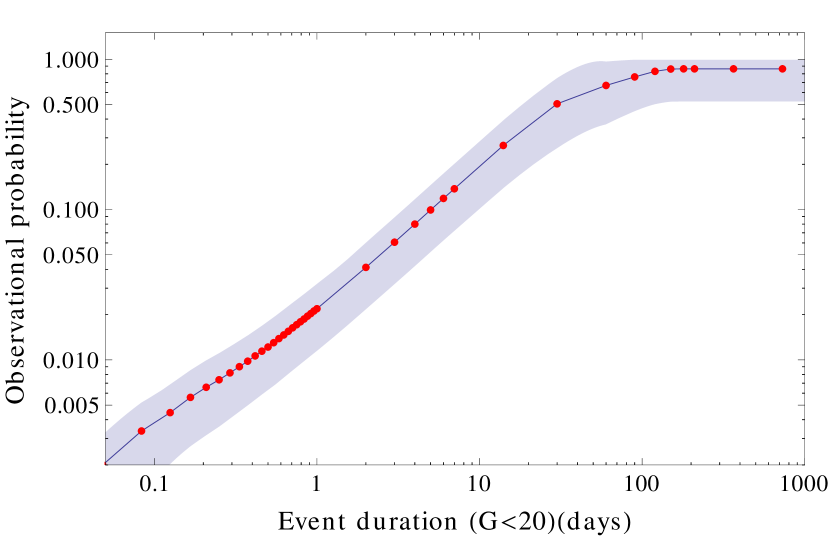
Figure 8: Probability for a transient event with duration $\Delta t$ to be observed by Gaia. $\Delta t$ is the time the event stays brighter than the Gaia limiting magnitude during the 5 years nominal mission.

4.1 Analysis

In accordance with upper limit showed in Fig. 1 and results from de Souza et al. (2011), we expect between $\sim 10^{2}-5\times 10^{3}$ events per year in all the sky. The uncertainties come from our poor understanding about the efficiency with which gas is converted into stars and GRBs are triggered (two unknown factors for Pop III stars). For a good statistics, we create a mock sample of $10^{5}$ events randomly generated by the Monte Carlo method in order to infer the PDF of an event to stay below $G=20$ over $\Delta t(\rm days)$. The average behavior for on-axis and off-axis afterglows as a function of $E_{iso}$ distribution is shown in Figs. 9-10. Once we have $P(\Delta t)$, we can generate a sample with $10^{4}$ events several times and test against their probability of being observed by Gaia, given by Fig. 8. Combining Figs. 8, 9, and 10, we obtain the following results for the average number of events observed during the five years of the Gaia mission:

• $E_{iso}\leqslant 5\times 10^{54}$

  on-axis:1.34 $\pm$ 0.62,
  off-axis: 1.26 $\pm$ 0.53,

• $E_{iso}\leqslant 10^{55}$

  on-axis: 2.78 $\pm$ 1.41,
  off-axis: 2.28 $\pm$ 0.88

Despite the fact that the total number of on-axis is always much lower than the number of off-axis, the observed number depends on assumptions regarding the GRB luminosity functions. For lower energies, the decrease in flux due to the observation angle leads to a larger number of light curves below the observational threshold. Thus, those on-axis have higher probability to be detected than those off-axis.

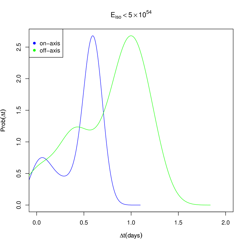
Figure 9: PDF of $\Delta t(days).$ Probability of an orphan afterglow with $E_{iso}\leqslant 5\times 10^{54}$ ergs to appear above the Gaia flux limit for a given time interval.

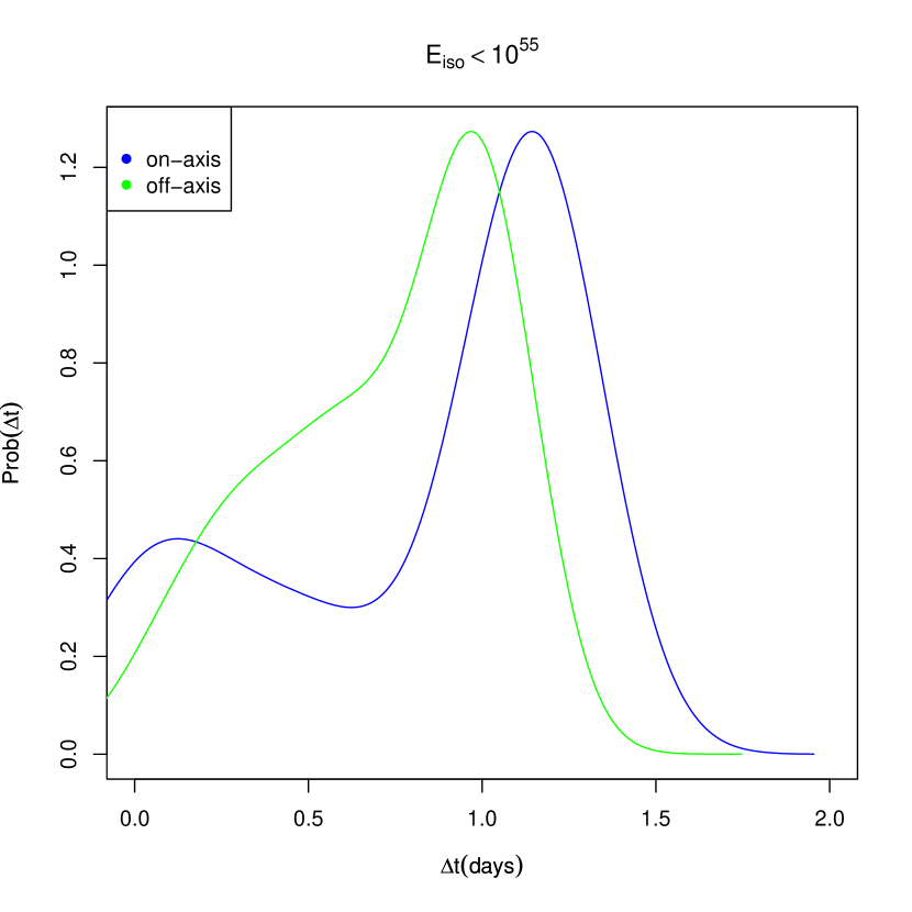
Figure 10: PDF of $\Delta t(days).$ Probability of an orphan afterglow with $E_{iso}\leqslant 10^{55}$ ergs to appear above the Gaia flux limit for a given time interval.

5 Discussion

Despite recent developments in theoretical studies on the formation of early generation of stars, there are no direct observations of Pop III stars yet. Following the suggestion that massive Pop III stars could trigger collapsar GRBs, we investigated the possibility to observe their OAs. We used previous results from the literature to estimate the SFR for Pop III.2 stars, including all relevant feedback effects: photo-dissociation, reionization, and metal enrichment.

Since we expect a larger number of OAs than on-axis GRBs, we estimated the possibility to observe such events during the five nominal operational years of the Gaia mission. The average number of events observed can be as high as to 2.28 $\pm$ 0.88 off-axis afterglows and 2.78 $\pm$ 1.41 for on-axis ones. This implies that among the possible afterglows observed by Gaia (Japelj & Gomboc 2011), a nonnegligible percentage ($\sim 10\%$) might belong to Pop III stars.

However, the detection of those events among the Gaia data will not be easy. Gaia will observe more than one billion objects all over the sky, and each object will be independently detected around eighty times during the mission, comprising a total of around $10^{12}$ astrometric, spectrophotometric, and spectroscopic observations (after detection, the observations are multiplexed in the focal plane). Consequently, finding the OAs events among all that data can be a quite challenging task.

In Gaia data processing, a system called AlertPipe is being implemented to deal with alerts of transient events. It is foreseen to operate as follows: first candidate alerts are classified using Gaia data, then sources are cross-matched with available catalogues through Virtual Observatory or local copies and further classified, and finally the alerts are stored on an alert server and released to the community as VOEvents (Hodgkin & Wyrzykowski 2011; van Leeuwen et al. 2011). Algorithms are under analysis for dealing with GRBs (Wyrzykowski, 2012 priv. comm.), but no performance figures are available at the present moment.

Based on Gaia data, the duration of the OA can be roughly estimated from the flux variation between two subsequent observations: if the event is detected during the transit of the first telescope, it will be re-observed 106.5 minutes later when Gaia’s second telescope re-observes the field. Moreover, the light curve will be sampled several times during the transit of each telescope, since at each column of Gaia’s focal plane an independent magnitude measurement will be performed (measurements are spaced by 4.4s).

The light curve alone may not be enough to distinguish between GRB afterglows and other optical transient sources, as noted by Japelj & Gomboc (2011). However, as these events have power law like SEDs and no quiescent counterpart, this information should also be considered. Further analysis of Gaia’s BP/RP low-dispersion spectrophotometry are needed to distinguish between different transients with similar characteristics. To perform transient event classification, AlertPipe uses several algorithms, including bayesian classifiers, template matching, and self-organizing maps (Hodgkin & Wyrzykowski 2010).

A possible way to search for such objects within a large survey is to look for signatures of afterglows from Pop III stars. Two important characteristics of these objects are the total energy of Pop III GRBs, which can be much higher than those of Pop I/II GRBs, and the active duration time of their jet, which can be much longer than Pop I/II GRB jets due to the larger progenitor star. Consequently, the detection of GRBs with very high $E_{iso}$ and very long duration could be indicative of such objects (Suwa & Ioka 2011; Toma et al. 2011). Thus, they should appear as quasi-steady point sources in the radio survey observations. But the indication should be complemented with the constraint on the metal abundances in the surrounding medium with high-resolution IR and X-ray spectroscopy. Since we do not have any observation of these objects, we have to rely on theoretical models to compare the data. A way to look for such objects that is worth future investigation is the use of automatic light curve classifiers, which are widely implemented for classifying supernovae and transients in general (Johnson & Crotts 2006; Kuznetsova & Connolly 2007; Poznanski et al. 2007; Rodney & Tonry 2009; Falck et al. 2010; Newling et al. 2011; Richards et al. 2011; Sako et al. 2011; Ishida & de Souza 2012). In principle, the theoretical model could work as a training set for the classifier, which would be then applied to surveys to identify possible candidates for further spectroscopical follow up.

These OAs event will be detected by the Gaia data processing pipeline just like any other transient. The timescales for raising the alerts are very dependent on specificities of the Gaia dataflow, but it is foreseen that, in the worst case, the data will be available for analysis by AlertPipe 24h after the observation. The alerts will thus be raised no later than 48h after the Gaia observation (Wyrzykowski & Hodgkin 2011). Nonetheless, it is not yet clear if AlertPipe by itself will be able to determine the nature of the transient as an OA.

Moreover, due to the design of the mission dataflow, real-time identification will not be possible, but further identification of OAs using data from satellites/telescopes operating on other wavelengths may be possible, as VOEvents will be created by the Gaia data processing alert system. Also, OAs could be identified if they trigger X-ray detectors, such as Swift’s BAT (Barthelmy et al. 2005), Fermi’s LAT (Atwood et al. 2009), which is foreseen to operate until 2018, or future instruments, such as SVOM (Schanne et al. 2010). Finally, the same may also be observed by other large-scale optical surveys on Earth, e.g., LSST (Ivezic et al. 2008) and Pan-STARRS (Kaiser et al. 2002), improving the sampling of the events’ light curve and providing information on other optical bands.

6 Conclusion

It is important to emphasize that our knowledge concerning first stars and their GRBs is still quite incomplete. Many of their properties (e.g., characteristic mass, SFR and efficiency to trigger GRBs) are still very uncertain, and more reliable information can only come once a detection is confirmed. Recently, Hosokawa et al. (2011), performing state-of-the-art radiation-hydrodynamics simulations, showed that the typical mass of primordial stars could be $\sim 43M_{\odot}$, i.e., less massive than originally expected by theoretical models. Their results, though, are affected by assumptions on the initial conditions. This confirms that we are far away from understanding all characteristics of these objects and any observation would be of paramount importance to improve theoretical models.

In this work, we estimated the average number of OAs events originating from Pop III stars that the Gaia mission may observe to be up to 2.28 $\pm$ 0.88 off-axis afterglows and 2.78 $\pm$ 1.41 on-axis ones. In case such events are found among Gaia data, valuable physical properties associated with the primordial stars of our Universe and their environment could be constrained.