On the Complexity of Solving Quadratic Boolean Systems

Abstract

A fundamental problem in computer science is to find all the common zeroes of $m$ quadratic polynomials in $n$ unknowns over $\mathbb{F}_{2}$. The cryptanalysis of several modern ciphers reduces to this problem. Up to now, the best complexity bound was reached by an exhaustive search in $4\log_{2}n\,2^{n}$ operations. We give an algorithm that reduces the problem to a combination of exhaustive search and sparse linear algebra. This algorithm has several variants depending on the method used for the linear algebra step. Under precise algebraic assumptions on the input system, we show that the deterministic variant of our algorithm has complexity bounded by $O(2^{0.841n})$ when $m=n$, while a probabilistic variant of the Las Vegas type has expected complexity $O(2^{0.792n})$. Experiments on random systems show that the algebraic assumptions are satisfied with probability very close to 1. We also give a rough estimate for the actual threshold between our method and exhaustive search, which is as low as 200, and thus very relevant for cryptographic applications.

1 Introduction

Motivation and Problem Statement. Solving multivariate quadratic polynomial systems is a fundamental problem in Information Theory. Moreover, random instances seem difficult to solve. Consequently, the security of several multivariate cryptosystems relies on its hardness, either directly (e.g., HFE [32], UOV [28],…) or indirectly (e.g., McEliece [20]). In some cases, systems of special types have to be solved, but recent proposals like the new Polly Cracker type cryptosystem [1] rely on the hardness of solving random systems of equations. This motivates the study of the complexity of generic polynomial systems. A particularly important case for applications in cryptology is the Boolean case; in that case both the coefficients and the solutions of the system are over $\mathbb{F}_{2}$. The main problem to be solved is the following:

The Boolean Multivariate Quadratic Polynomial Problem (Boolean MQ)
Input: $(f_{1},\ldots,f_{m})\in\mathbb{F}_{2}[x_{1},\ldots,x_{n}]^{m}$ with $\deg(f_{i})=2$ for $i=1,\dots,m$.
Question: Find – if any – all $z\in\mathbb{F}_{2}^{n}$ such that $f_{1}(z)=\cdots=f_{m}(z)=0$.

Another related problem stems from the fact that in many cryptographic applications, it is sufficient to find at least one solution of the corresponding polynomial system (in that case a solution is the original clear message or is related to the secret key). For instance, the stream cipher QUAD [6, 7] relies on the iteration of a set of multivariate quadratic polynomials over $\mathbb{F}_{2}$ so that the security of the keystream generation is related to the difficulty of finding at least one solution of the Boolean MQ problem. Thus, we also consider the following variant of the Boolean MQ problem:

The Boolean Multivariate Quadratic Polynomial Satisfiability Problem (Boolean MQ SAT)
Input: $(f_{1},\ldots,f_{m})\in\mathbb{F}_{2}[x_{1},\ldots,x_{n}]^{m}$ with $\deg(f_{i})=2$ for $i=1,\dots,m$.
Question: Find – if any – one $z\in\mathbb{F}_{2}^{n}$ such that $f_{1}(z)=\cdots=f_{m}(z)=0$.

Testing for the existence of a solution is an NP-complete problem (it is plainly in NP and 3-SAT can be reduced to it [22]). Clearly, the Boolean MQ problem is at least as hard as Boolean MQ SAT, while an exponential complexity is achieved by exhaustive search.

Throughout this paper, random means distributed according to the uniform distribution (given $m$ and $n$, a random quadratic polynomial is uniformly distributed if all its coefficients are independently and uniformly distributed over $\mathbb{F}_{2}$). The relation between the difficulties of Boolean MQ and Boolean MQ SAT depends on the relative values of $m$ and $n$. When $m>n$, the number of solutions of the algebraic system is 0 or 1 with large probability and thus finding one or all solutions is very similar, while when $m=n$, the probability that a random system has at least one solution over $\mathbb{F}_{2}$ tends to $1-\frac{1}{e}\approx 0.63$ for large $n$ [24]. Hence if we have to find a least one solution of a system with $m<n$ equations in $n$ variables it is enough to specialize $n-m$ variables randomly in $\mathbb{F}_{2}$; the resulting system has at least one solution with limit probability $0.63$ and is easier to solve (since the number of equations and variables is only $m$). Consequently, in the remainder of this article we restrict ourselves to the case $m\geq n$.

To the best of our knowledge, in the worst case, the best complexity bound to solve the Boolean MQ problem is obtained by a modified exhaustive search in $4\log_{2}(n)2^{n}$ operations [10]. Being able to decrease significantly this complexity is a long-standing open problem and is the main goal of this article. It is crucial for practical applications to have sharp estimates of the asymptotic complexity: it is especially important in the cryptographic context where this value may have a strong impact on the sizes of the keys needed to reach a given level of security.

Main results. We describe a new algorithm BooleanSolve that solves Boolean MQ for determined or overdetermined systems ($m=\alpha n$ with $\alpha\geq 1$). We show how to adapt it to solve the Boolean MQ SAT problem. This algorithm has deterministic and Las Vegas variants, depending on the choice of some linear algebra subroutines. Our main result is:

Theorem 1.

The Boolean MQ Problem is solved by Algorithm BooleanSolve. If $m=n$ and the system fulfills algebraic assumptions detailed in Theorem 2, then this algorithm uses a number of arithmetic operations in ${\mathbb{F}}_{2}$ that is:

• $O(2^{0.841n})$ using the deterministic variant;

• of expectation $O(2^{0.792n})$ using the Las Vegas probabilistic variant.

Recall that for a probabilistic algorithm of the Las Vegas type, the result is always correct, but the complexity is a random variable. Here its expectation is controlled well.

Outline. Our algorithm is a variant of the hybrid approach by [8, 9]: we specialize the last $k$ variables to all possible values, and check the consistency of the specialized overdetermined systems $(\tilde{f}_{1},\dots,\tilde{f}_{m})$ in the remaining variables $x_{1},\dots,x_{\ell}$.

This consistency check is done by searching for polynomials $h_{1},\dots,h_{m+\ell}$ in $x_{1},\dots,x_{\ell}$ such that

$$h_{1}\tilde{f}_{1}+\dots+h_{m}\tilde{f}_{m}+h_{m+1}x_{1}(1-x_{1})+\dots+h_{m+\ell}x_{\ell}(1-x_{\ell})=1.$$ (1)

If such polynomials exist then obviously the system is not consistent. Given a bound $d$ on the degrees of the polynomials $h_{i}\tilde{f}_{i}$ and $h_{m+i}x_{i}(1-x_{i})$, the existence of the $h_{i}$ can be checked by linear algebra. The corresponding matrix is known as the Macaulay matrix in degree $d$. It is a matrix whose rows contain the coefficients of the polynomials $\tilde{f}_{i}$ and $x_{i}(1-x_{i})$ multiplied by all monomials of degree at most $d-2$, each column corresponding to a monomial of degree at most $d$. Taking into account the special shape of the polynomials $x_{i}(1-x_{i})$ leads to a more compact variant that we call the boolean Macaulay matrix (see Section 2).

When linear algebra on the Macaulay matrix in degree $d$ produces a solution of (1), the corresponding $h_{i}$’s give a certificate of inconsistency. Otherwise, our algorithm proceeds with an exhaustive search in the remaining variables. In summary, our algorithm is a partial exhaustive search where the Macaulay matrices permit to prune branches of the search tree. The correctness of the algorithm is clear.

The key point making the algorithm efficient is the choice of $k$ and $d$. If $d$ is large, then the cost of the linear algebra stage becomes high. If $d$ is small, the matrices are small, but many branches with no solutions are not pruned and require an exhaustive search. This is where we use the relation between the Macaulay matrix and Gröbner bases. We define a witness degree $\operatorname{d_{wit}}$, which has the property that any polynomial in a minimal Gröbner basis of the system is obtained as a linear combination of the rows of the Macaulay matrix in degree $\operatorname{d_{wit}}$. Hilbert’s Nullstellensatz states that the system has no solution if and only if $1$ belongs to the ideal generated by the polynomials, which implies that 1 is a linear combination of the rows of the Macaulay matrix in degree $\operatorname{d_{wit}}$, making $\operatorname{d_{wit}}$ an upper bound for the choice of $d$ in (1).

Our complexity estimates rely on a good control of the witness degree. For a homogeneous polynomial ideal, the classical Hilbert function of the degree $d$ is the dimension of the vector space obtained as the quotient of the polynomials of degree $d$ by the polynomials of degree $d$ in the ideal. The witness degree is bounded by the first degree where the Hilbert function of the ideal generated by the homogenized equations is 0. Under the algebraic assumption of boolean semi-regularity (see Definition 7), we obtain an explicit expression for the generating series of the Hilbert function, known as the Hilbert series of the ideal. From there, in Proposition 7, using the saddle-point method as in [4, 5, 3], we show that when $m=\alpha n$ and $n\rightarrow\infty$, the witness degree behaves like ${\operatorname{d_{wit}}}\leq c_{\alpha}n$ for a constant $c_{\alpha}$ that we determine explicitly. Informally, boolean semi-regularity amounts to demanding a “sufficient” independence of the equations. In the case of infinite fields, a classical conjecture by [23] states that generic systems are semi-regular. In our context where the field is $\mathbb{F}_{2}$, we give strong experimental evidence (Section 4.1) that for $n$ sufficiently large, boolean semi-regularity holds with probability very close to 1 for random systems. Thus, our complexity estimates for boolean semi-regular systems apply to a large class of systems in practice.

Once the witness degree is controlled, the size of the Macaulay matrix depends only on the choice of $k$ and the optimal choice depends on the complexity of the linear algebra stage. In the Las Vegas version of Algorithm BooleanSolve, we exploit the sparsity of this matrix by using a variant of Wiedemann’s algorithm [25] (following [40, 27, 39]) for solving singular linear systems. In the deterministic version, we do not know of efficient ways to take advantage of the sparsity of the matrix, whence a slightly higher complexity bound. We can then draw conclusions and obtain a complexity estimate of the algorithm depending on $k/n$ and $n$ (Proposition 8). The optimal value for $k$ is $\simeq 0.45\,n$ in the Las Vegas setting and $\simeq 0.59\,n$ in the deterministic variant, completing the proof of our main theorem.

The complexity analysis is especially important for practical applications in multivariate Cryptology based on the Boolean MQ problem, since it shows that in order to reach a security of $2^{s}$ (with $s$ large), one has to construct systems of boolean quadratic equations with at least $s/0.7911\simeq 1.264s$ variables.

Related works. Due to its practical importance, many algorithms have been designed to solve the MQ problem in a wide range of contexts. First, generic techniques for solving polynomial systems can be used. In particular, Gröbner basis algorithms (such as Buchberger’s algorithm [11], $F_{4}$ [16], $F_{5}$ [17], and FGLM [18]) are well suited for this task. For instance, the $F_{5}$ algorithm has broken several challenges of the HFE public-key cryptosystem [19]. In the cryptanalysis context, the XL algorithm [29] (which can be seen as a variant of Gröbner basis algorithms [2]) has given rise to a large family of variants. All these techniques are closely related to the Macaulay matrix, introduced by [30] as a tool for elimination. In order to reduce the cost of linear algebra for the efficient computation of the resultant of multivariate polynomial systems, the idea of using Wiedemann’s algorithm on the Macaulay matrix has been proposed by [12]; however since the specificities of the Boolean case are not taken into account, the complexity of applying [12] to quadratic equations is $O(2^{4\,n})$.

[41] propose a heuristic analysis of the FXL algorithm leading them to an upper bound $O(2^{0.875n})$ for the complexity of solving the MQ problem over $\mathbb{F}_{2}$. In particular, they give an explicit formula for the Hilbert series of the ideal generated by the polynomials. However, the exact assumptions that have to be verified by the input systems are unclear. Also, similar results have been announced in [42, Section 2.2], but the analysis there relies on algorithmic assumptions (e.g., row echelon form of sparse matrices in quadratic complexity) that are not known to hold currently. Under these assumptions, the authors show that the best trade-off between exhaustive search and row echelon form computations in the FXL algorithm is obtained by specializing $0.45n$ variables. This is the same value we obtain and prove with our algorithm. Also, a limiting behavior of the cost of the hybrid approach is obtained in [9] when the size of the finite field is big enough; these results are not applicable over $\mathbb{F}_{2}$.

Other algorithms have been proposed when the system has additional structural properties. In particular, the Boolean MQ problem also arises in satisfiability problems, since boolean quadratic polynomials can be used for representing constraints. In these contexts, the systems are sparse and for such systems of higher degree the $2^{n}$ barrier has been broken [33, 34]; similar results also exist for the $k$-SAT problem. Our algorithm does not exploit the extra structure induced by this type of sparsity and thus does not improve upon those results.

Organization of the article. The main algorithm and the algebraic tools that are used throughout the article are described in Section 2. Then a complexity analysis is performed in Section 3 by studying the asymptotic behaviour of the witness degree and the sizes of the Macaulay matrices involved, under algebraic assumptions. In Section 4, we provide a conjecture and strong experimental evidence that these algebraic assumptions are verified with probability close to $1$ for $n$ sufficiently large. Finally, in Section 5 we propose an extension of the main algorithm that improves the quality of the linear filtering when $n$ is small. We also show how the complexity results from Section 3 can be applied to the cryptosystem QUAD, leading to an evaluation of the sizes of the parameters needed to reach a given level of security.

2 Algorithm

Notations. Let $m$ and $n$ be two positive integers and let $R$ be the ring $\mathbb{F}_{2}[x_{1},\ldots,x_{n}]$. In the following, the notation $\mathsf{Monomials}(d)$ stands for the set of monomials in $R$ of degree at most $d$.

Since we are looking for solutions of the system in $\mathbb{F}_{2}$ (and not in its algebraic closure), we have to take into account the relations $x_{i}^{2}-x_{i}=0$. Therefore, we consider the application $\varphi$ mapping a monomial to its square-free part ($\varphi(\prod_{i=1}^{n}x_{i}^{a_{i}})=\prod_{i=1}^{n}x_{i}^{\min(a_{i},1)}$) and extended to $R$ by linearity.

If $(f_{1},\ldots,f_{m})\in\mathbb{F}_{2}[x_{1},\ldots,x_{n}]^{m}$ is a system of polynomials, its homogenization is denoted by the system $(f_{1}^{(h)},\ldots,f_{m}^{(h)})\in\mathbb{F}_{2}[x_{1},\ldots,x_{n},h]$ and is defined by

$$f_{i}^{(h)}(x_{1},\ldots,x_{n},h)=h^{\deg{(f_{i})}}f_{i}\left(\frac{x_{1}}{h},\ldots,\frac{x_{n}}{h}\right).$$

In the sequel, we consider the classical grevlex monomial ordering (graded reverse lexicographical), as defined for instance in [14, §2.2, Defn. 6]. Also, if $f$ is a polynomial, $\operatorname{LM}(f)$ denotes its leading monomial for that order. If $I$ is an ideal, then $\operatorname{LM}(I)$ denotes the ideal generated by the leading monomials of all polynomials in $I$.

2.1 Macaulay matrix

Definition 1.

Let $(f_{1},\ldots,f_{m})$ be polynomials in $R$. The boolean Macaulay matrix in degree $d$ (denoted by $\mathsf{Macaulay}(d)$) is the matrix whose rows contain the coefficients of the polynomials $\{\varphi(tf_{j})\}$ where $1\leq j\leq m$, $t$ is a squarefree monomial, and $\deg(tf_{j})=d$. The columns correspond to the squarefree monomials in $R$ of degree at most $d$ and are ordered in descending order with respect to the grevlex ordering. The element in the row corresponding to $\varphi(tf_{j})$ and the column corresponding to the monomial $m$ is the coefficient of $m$ in the polynomial $\varphi(tf_{j})$.

Note that the boolean Macaulay matrix can be obtained as a submatrix of the classical Macaulay matrix of the system $\langle f_{1},\ldots,f_{m},x_{1}^{2}-x_{1},\ldots,x_{n}^{2}-x_{n}\rangle$ after Gaussian reduction by the rows corresponding to the polynomials $(x_{1}^{2}-x_{1},\ldots,x_{n}^{2}-x_{n})$.

Lemma 1.

Let $\mathsf{M}$ be the $r_{\mathsf{Mac}}\times c_{\mathsf{Mac}}$ boolean Macaulay matrix of the system $(f_{1},\ldots,f_{m})$ in degree $d$. Let $\mathbf{r}$ denote the $1\times c_{\mathsf{Mac}}$ vector $\mathbf{r}=(0,\dots,0,1)$. If the linear system $\mathbf{u}\cdot\mathsf{M}=\mathbf{r}$ has a solution, then the system $f_{1}=\dots=f_{m}=0$ has no solution in $\mathbb{F}_{2}^{n}$.

Proof.

If the system $\mathbf{u}\cdot\mathsf{M}=\mathbf{r}$ has a solution, then there exists a linear combination of the rows of the Macaulay matrix which yields the constant polynomial $1$. Therefore, $1\in\langle f_{1},\ldots,f_{m},x_{1}^{2}-x_{1},\ldots,x_{n}^{2}-x_{n}\rangle$. ∎

2.2 Witness degree

We consider an indicator of the complexity of affine polynomial systems: the witness degree. It has the property that a Gröbner basis of the ideal generated by the polynomials can be obtained by performing linear algebra on the Macaulay matrix in this degree. In particular, if the system has no solution, then the witness degree is closely related to the classical effective Nullstellensatz (see e.g., [26]).

Definition 2.

Let $\mathbf{F}=(f_{1},\ldots,f_{m},x_{1}^{2}-x_{1},\ldots,x_{n}^{2}-x_{n})$ be a sequence of polynomials and $I=\langle\mathbf{F}\rangle$ the ideal it generates. Denote by $I_{\leq d}$ and by $J_{\leq d}$ the $\mathbb{F}_{2}$-vector spaces defined by

$$\begin{array}[]{rccl}I_{\leq d}&=&\{p\mid&p\in I,\deg(p)\leq d\},\\ J_{\leq d}&=&\{p\mid&\exists h_{1},\ldots,h_{m+n},\forall i\in\{1,\ldots,m+n\},\deg(h_{i})\leq d-2,\\ &&&p=\sum_{i=1}^{m}h_{i}f_{i}+\sum_{j=1}^{n}h_{m+j}(x_{j}^{2}-x_{j})\}.\end{array}$$

We call witness degree $(\operatorname{d_{wit}})$ of $\mathbf{F}$ the smallest integer $d_{0}$ such that $I_{\leq d_{0}}=J_{\leq d_{0}}$ and $\langle\{\operatorname{LM}(f)\mid f\in I_{\leq d_{0}}\}\rangle=\operatorname{LM}(I)$.

Consider a row echelon form of the boolean Macaulay matrix in degree $d$ of the system $(f_{1},\dots,f_{m})$ of polynomials. Then the first nonzero element of each row corresponds to a leading monomial of an element of $I$, belonging to $\operatorname{LM}(I)$. For large enough $d$, Dickson’s lemma [14, §2.4, Thm. 5] implies that the collection of those monomials up to degree $d$ generates $\operatorname{LM}(I)$ and thus the polynomials corresponding to those rows together with $\{x_{1}^{2}-x_{1},\ldots,x_{n}^{2}-x_{n}\}$ form a Gröbner basis of $I$ with respect to the grevlex ordering. Another interpretation of the witness degree is that it is precisely the smallest such $d$.

2.3 Algorithm

Algorithm 1 BooleanSolve

1:$m,n,k\in\mathbb{N}$ such that $m\geq n>k$ and $f_{1},\ldots,f_{m}$ quadratic polynomials in $\mathbb{F}_{2}[x_{1},\ldots,x_{n}]$.

2:The set of boolean solutions of the system $f_{1}=\dots=f_{m}=0$.

3:$S:=\emptyset$.

4:${d_{0}}:=$ index of the first nonpositive coefficient in the series expansion at 0 of the rational function $\frac{(1+t)^{n-k}}{(1-t)(1+t^{2})^{m}}$.

5:for all $(a_{n-k+1},\ldots,a_{n})\in\mathbb{F}_{2}^{k}$ do

6:     for $i$ from $1$ to $m$ do

7:         $\tilde{f}_{i}(x_{1},\ldots,x_{n-k}):=f_{i}(x_{1},\ldots,x_{n-k},a_{n-k+1},\ldots,a_{n})\in\mathbb{F}_{2}[x_{1},\ldots,x_{n-k}]$.

8:     end for

9:     $\mathsf{M}:=$ boolean Macaulay matrix of $(\tilde{f}_{1},\ldots,\tilde{f}_{m})$ in degree ${d_{0}}$.

10:     if the system $\mathbf{u}\cdot\mathsf{M}=\mathbf{r}$ is inconsistent then$\triangleright$ $\mathbf{r}$ as defined in Lemma 1

11:         $T:=$ solutions of the system ($\tilde{f}_{1}=\cdots=\tilde{f}_{m}=0$) (exhaustive search).

12:         for all $(t_{1},\ldots,t_{n-k})\in T$ do

13:              $S:=S\cup\{(t_{1},\ldots,t_{n-k},a_{n-k+1},\ldots,a_{n})\}$.

14:         end for

15:     end if

16:end for

17:return $S$.

Our algorithm is given in Algorithm 1. The general principle is to perform an exhaustive search in two steps, using a test of consistency of the Macaulay matrix to prune most of the branches of the second step of the search.

When the system $\mathbf{u}\cdot\mathsf{M}=\mathbf{r}$ is consistent, the corresponding branch of the searching tree is not explored. In that case, by Lemma 1, any solution of the linear system $\mathbf{u}\cdot\mathsf{M}=\mathbf{r}$ can be used as a certificate that there exists no solution of the polynomial system $f_{1}=\dots=f_{m}=0$ in this branch.

Proposition 1.

Algorithm BooleanSolve is correct and solves the Boolean MQ problem.

Proof.

By Lemma 1, if the test in line 8 finds the linear system to be consistent, then there can be no solution with the given values of $(a_{n-k+1},\dots,a_{n})$. Otherwise, the exhaustive search proceeds and cannot miss a solution. It is important to note that the choice of the actual value ${d}_{0}$ does not have any impact on the correctness of the algorithm. ∎

Algorithm BooleanSolve is easily be adapted to solve the Boolean MQ  SAT problem by replacing lines 9-12 of the previous algorithm by:

9:$T:=$ at least one solution of the system ($\tilde{f}_{1}=\cdots=\tilde{f}_{m}=0$) (modified exhaustive search).

10:if $T\neq\emptyset$ then

11:     return $\{(t_{1},\ldots,t_{n-k},a_{n-k+1},\ldots,a_{n})\mid(t_{1},\ldots,t_{n-k})\in T\}$

12:end if

2.4 Testing Consistency of Sparse Linear Systems

The choice of the algorithm to test whether the sparse linear system $\mathbf{u}\cdot\mathsf{M}=\mathbf{r}$ is consistent or not is crucial for the efficiency of Algorithm BooleanSolve. A simple deterministic algorithm consists in computing a row echelon form of the matrix: the linear system is consistent if and only if the last nonzero row of the row echelon form is equal to the vector $\mathbf{r}$. We show in Section 3 that this is sufficient to pass below the $2^{n}$ complexity barrier. We recall for future use the complexity of this method.

Proposition 2 ([36], Proposition 2.11).

The row echelon form of an $N\times M$ matrix over a field $k$ can be computed in $O(NMr^{\theta-2})$ arithmetic operations in $k$, where $r$ is the rank of the matrix and $\theta\leq 3$ is such that any two $n\times n$ matrices over $k$ can be multiplied in $O(n^{\theta})$ arithmetic operations in $k$.

Here, $\theta=3$ is the cost of classical matrix multiplication and in this case a simple Gaussian reduction to row echelon form is sufficient. The best known value for $\theta$ has been 2.376 for a long time, by a result of [13]. Recent improvements of that method by [37, 38] have decreased it to 2.3727, but this does not have a significant impact on our analysis.

This result does not exploit the sparsity of Macaulay matrices. We do not know of an efficient deterministic algorithm for row reduction that exploits this sparsity. Instead, we use an efficient Las Vegas variant of Wiedemann’s algorithm due to [25], whose specification is summarized in Algorithm TestConsistency. In this algorithm, the matrix $A$ is given by two black boxes performing the operations $x\mapsto Ax$ and $u\mapsto A^{t}u$. The complexity is expressed in terms of the number of evaluations of these black boxes, which in our context will each have a cost bounded by the number of nonzero coefficients of Macaulay matrices. The algorithm is presented in [25] for matrices with entries in an arbitrary field. We specialize it here in the case where the field is $\mathbb{F}_{2}$. The key ideas are a preconditioning of the matrix by multiplying it by random Toeplitz matrices and working in a suitable field extension to get access to sufficiently many points for picking random elements.

Algorithm 2 TestConsistency [25]

1:

• A black box for $\mathbf{x}\mapsto\mathsf{A}\cdot\mathbf{x}$, where $\mathsf{A}\in\mathbb{K}^{N\times N}$.

• A black box for $\mathbf{u}\mapsto\mathsf{A}^{t}\cdot\mathbf{u}$.

• $\mathbf{b}\in\mathbb{K}^{N\times 1}$.

2:

• (“consistent”,$\mathbf{x}$) with $\mathsf{A}\cdot\mathbf{x}=\mathbf{b}$ if the system has a solution

• (“inconsistent”,$\mathbf{u}$) if the system does not have a solution, with $\mathbf{u}^{t}\cdot\mathsf{A}=0$ and $\mathbf{u}^{t}\cdot\mathbf{b}\neq 0$, certifying the inconsistency.

Proposition 3 ([25]).

Algorithm 2 determines the consistency of an $N\times N$ matrix with expected complexity $O(N\log N)$ evaluations of the black boxes and $O(N^{2}\log^{2}N\log\log N)$ additional operations in $\mathbb{F}_{2}$.

Macaulay matrices are rectangular. We therefore first make them square by padding with zeroes. The complexity estimate is then used with $N$ the maximum of the row and column dimensions of the matrices.

3 Complexity Analysis

Algorithm BooleanSolve deals with a large number of Macaulay matrices in degree $d_{0}$. We first obtain bounds on the row and column dimensions of Macaulay matrices, as well as their number of nonzero entries, in terms of the degree. We then bound the witness degree by $d_{0}$. The complexity analysis is concluded by optimizing the value of the ratio $k/n$ that governs the number of variables evaluated in the first exhaustive search.

3.1 Sizes of Macaulay Matrices

Proposition 4.

Let $(f_{1},\dots,f_{m})$ be quadratic polynomials in ${\mathbb{F}}_{2}[x_{1},\dots,x_{n}]$. Denote by $r_{\mathsf{Mac}}$ (resp. $c_{\mathsf{Mac}}$, $s_{\mathsf{Mac}}$) the number of rows (resp. columns, number of nonzero entries) of the associated boolean Macaulay matrix in degree $d$. If $1\leq d<n/2$, then

$$c_{\mathsf{Mac}}<\frac{1-x}{1-2x}\binom{n}{d},\,\,r_{\mathsf{Mac}}<{m}\frac{x^{2}}{(1-2x)(1-x)}\binom{n}{d},\,\,s_{\mathsf{Mac}}<{mn^{2}}\frac{x^{2}}{(1-2x)(1-x)}\binom{n}{d},$$ (2)

where $x=d/n$.

Proof.

The number of columns of the boolean Macaulay matrix is simply the number of squarefree monomials of degree at most $d$ in $n$ variables. The number of rows is that same number of monomials for degree $d-2$, multiplied by the number $m$ of polynomials. Finally, each row corresponding to a polynomial $f_{i}$ has a number of nonzero entries bounded by the number of squarefree monomials of degree at most 2 in $n$ variables. Standard combinatorial counting thus gives

$$c_{\mathsf{Mac}}=\sum_{i=0}^{d}{\binom{n}{i}},\qquad r_{\mathsf{Mac}}=m\sum_{i=0}^{d-2}{\binom{n}{i}},\qquad s_{\mathsf{Mac}}\leq\left(1+n+\binom{n}{2}\right)r_{\mathsf{Mac}}\leq n^{2}r_{\mathsf{Mac}},$$ (3)

where in the last inequality we use the fact that $n\geq 2$. Now, the bounds come from a well-known inequality on binomial coefficients: for $0\leq d<n/2$,

$$\sum_{i=0}^{d}{\binom{n}{i}}<\frac{1}{1-d/(n-d)}\binom{n}{d}.$$

Indeed, the sequence $\binom{n}{i}$ is increasing for $0\leq i\leq n/2$. Factoring out $\binom{n}{d}$ leaves a sum that is bounded by the geometric series $1+d/(n-d)+\dotsb$. This gives the bound for $c_{\mathsf{Mac}}$. The bound for $r_{\mathsf{Mac}}$ is obtained by evaluating this bound at $d-2$, writing $\binom{n}{d-2}$ as a rational function times $\binom{n}{d}$ and finally bounding $x(x-1/n)/((1-2x+4/n)((1-x)+1/n))$ by $x^{2}/((1-2x)(1-x))$. ∎

3.2 Bound on the Witness Degree of Inconsistent Systems

First, we prove that the witness degree can be upper bounded by the so-called degree of regularity of the homogenized system. Here and subsequently, we call dimension of an ideal $I\subset R$ the Krull dimension of the quotient ring $R/I$ (see e.g., [15, §8]).

Definition 3.

The degree of regularity $\operatorname{d_{reg}}(I)$ of a homogeneous ideal $I$ of dimension $0$ is defined as the smallest integer $d$ such that all homogeneous polynomials of degree $d$ are in $I$.

Proposition 5.

Let $\mathbf{F}=\left(f_{1},\ldots,f_{m},x_{1}^{2}-x_{1},\ldots,x_{n}^{2}-x_{n}\right)$ be a sequence of polynomials such that the system $\mathbf{F}=0$ has no solution. Then the ideal generated by the homogenized system

$$I^{(h)}=\left\langle f_{1}^{(h)},\ldots,f_{m}^{(h)},x_{1}^{2}-x_{1}h,\ldots,x_{n}^{2}-x_{n}h\right\rangle$$

has dimension $0$ and $\operatorname{d_{wit}}(\mathbf{F})\leq\operatorname{d_{reg}}(I^{(h)})$.

Proof.

By Hilbert’s Nullstellensatz, the ideal $I$ generated by $\mathbf{F}$ contains $1$ (hence $1$ is a Gröbner basis of $I$). Therefore, there exists $\alpha\in\mathbb{N}\setminus\{0\}$ such that $h^{\alpha}\in I^{(h)}$. Consequently, for the grevlex ordering, $\langle x_{1}^{2},\ldots,x_{n}^{2},h^{\alpha}\rangle\subset\operatorname{LM}(I^{(h)})$ and thus the dimension of $\operatorname{LM}(I^{(h)})$ is $0$. As a consequence (see [14, §9.3, Prop. 9]), $\dim(I^{(h)})=\dim(\operatorname{LM}(I^{(h)}))=0$.

Let $G^{(h)}$ be a minimal Gröbner basis of the homogenized ideal $I^{(h)}$ for the grevlex ordering. By definition of the degree of regularity, there exist polynomials $\ell_{i}$ and $\ell^{\prime}_{j}$ such that $h^{\operatorname{d_{reg}}(I^{(h)})}=\sum_{1\leq i\leq m}f_{i}^{(h)}\ell_{i}+\sum_{1\leq j\leq n}(x_{j}^{2}-x_{j}h)\ell^{\prime}_{j}$. The ideal $I^{(h)}$ being homogeneous, it is possible to find such a combination with $\deg(f_{i}^{(h)}\ell_{i})\leq\operatorname{d_{reg}}(I^{(h)}),\deg((x_{j}^{2}-x_{j}h)\ell^{\prime}_{j})\leq\operatorname{d_{reg}}(I^{(h)})$ for all $i,j$. Evaluating this identity at $h=1$ shows that $1$ belongs to the vector space generated by the rows of the boolean Macaulay matrix in degree $\operatorname{d_{reg}}(I^{(h)})$. ∎

Next, the degree of regularity can be obtained from the classical Hilbert series.

Definition 4.

Let $R^{(h)}$ be the ring $\mathbb{F}_{2}[x_{1},\ldots,x_{n},h]$, and let $R^{(h)}_{d}$ be the vector space of homogeneous polynomials of degree $d$. Also, for $I\subset R^{(h)}$ a homogeneous ideal, let $I_{d}$ denote the vector space defined by $I_{d}=R^{(h)}_{d}\cap I$. The Hilbert function $\mathsf{HF}_{I}$ and the Hilbert series $\mathsf{HS}_{I}$ of $I$ are defined by

$$\mathsf{HF}_{I}(d)=\dim(R^{(h)}_{d}/I_{d}),\hskip 45.52458pt\mathsf{HS}_{I}(t)=\sum_{i=0}^{\infty}\mathsf{HF}_{I}(d)t^{d}.$$

In view of the definition of the degree of regularity, if $I$ is a zero-dimensional ideal of $R^{(h)}$, then $\mathsf{HS}_{I}(t)$ is a polynomial of degree $\operatorname{d_{reg}}(I)-1$.

The next step is to obtain information on the Hilbert series for a large class of systems. To this end, we consider the so-called syzygy module, which describes the algebraic relations between the polynomials of a system.

Definition 5.

Let $(g_{1},\ldots,g_{\ell})\in(R^{(h)})^{\ell}$ be a polynomial system. A syzygy of $(g_{1},\ldots,g_{\ell})$ is a $\ell$-tuple $(s_{1},\ldots,s_{\ell})\in(R^{(h)})^{\ell}$ such that $\sum_{i=1}^{\ell}s_{i}g_{i}=0.$ The set of all syzygies of $(g_{1},\ldots,g_{\ell})$ is a submodule of $(R^{(h)})^{\ell}$. The degree of a syzygy $\mathbf{s}=(s_{1},\ldots,s_{\ell})$ is defined as $\deg(\mathbf{s})=\max_{1\leq i\leq\ell}\deg(g_{i}s_{i})$.

Obviously, for any such polynomial system, commutativity induces syzygies of the type

$$g_{i}g_{j}-g_{j}g_{i}=0.$$ (4)

Moreover, for any constant $a\in\mathbb{F}_{2}$ we have the relation $a^{2}=a$, thus expanding the square of a polynomial $\sum_{\alpha\in\mathbb{N}^{k}}a_{\alpha}\mathbf{x}^{\alpha}\in\mathbb{F}_{2}[x_{1},\ldots,x_{k}]$ gives $\sum_{\alpha\in\mathbb{N}^{k}}a_{\alpha}\mathbf{x}^{2\alpha}$. As a consequence, for a homogeneous quadratic polynomial $f_{i}^{(h)}=\sum_{1\leq j,k\leq n}a_{j,k}\,x_{j}x_{k}+\sum_{1\leq j\leq n}b_{j}\,x_{j}h+c\,h^{2}\in\mathbb{F}_{2}[x_{1},\ldots,x_{n},h]$, we obtain the following syzygy of the system $(f_{i}^{(h)},x_{1}^{2}-x_{1}h,\dots,x_{n}^{2}-x_{n}h)$:

$$(f_{i}^{(h)}-h^{2})f_{i}^{(h)}+\sum_{1\leq j,k\leq n}a_{j,k}\left(x_{k}^{2}(x_{j}^{2}-x_{j}h)+x_{j}h(x_{k}^{2}-x_{k}h)\right)+\sum_{1\leq j\leq n}b_{j}h^{2}(x_{j}^{2}-x_{j}h)=0.$$ (5)

Definition 6.

Let $\mathbf{F}^{(h)}=(f_{1}^{(h)},\dots,f_{n}^{(h)},x_{1}^{2}-x_{1}h,\dots,x_{n}^{2}-x_{n}h)$ be a system of homogeneous quadratic polynomials over $\mathbb{F}_{2}$. We call trivial syzygies of $\mathbf{F}^{(h)}$ and note $Syz_{\text{triv}}$ the module generated by the syzygies of types (4) and (5).

Definition 7.

A boolean homogeneous system $(f_{1}^{(h)},\ldots,f_{m}^{(h)})$ is called

• boolean semi-regular in degree $D$ if any syzygy whose degree is less than $D$ belongs to $Syz_{\text{triv}}$;

• boolean semi-regular if it is boolean semi-regular in degree $\operatorname{d_{reg}}(\langle f_{1}^{(h)},\ldots,f_{m}^{(h)},x_{1}^{2}-x_{1}h,\ldots,x_{n}^{2}-x_{n}h\rangle)$.

(This notion is slightly different from the semi-regularity over $\mathbb{F}_{2}$ defined in [4, 5].)

In the sequel we use the following notations: if $S\in\mathbb{Z}[[t]]$ is a power series, then $[S]$ denotes the series obtained by truncating $S$ just before the index of its first nonpositive coefficient. Also, $[t^{d}]S(t)$ denotes the coefficient of $t^{d}$ in $S$.

Proposition 6.

Let $(f_{1}^{(h)},\ldots,f_{m}^{(h)})$ be a boolean homogeneous system. Let $D_{0}$ denote the degree of regularity of the system $(f_{1}^{(h)},\ldots,f_{m}^{(h)},x_{1}^{2}-x_{1}h,\ldots,x_{n}^{2}-x_{n}h)$. If the systems $(f_{1}^{(h)},\ldots,f_{i-1}^{(h)},f_{i}^{(h)}-h^{2})$ and $(f_{1}^{(h)},\ldots,f_{i-1}^{(h)},f_{i}^{(h)})$ are $D_{0}-2$ (resp. $D_{0}$)-boolean semi-regular for each $i\in\{2,\ldots,m\}$, then the Hilbert series of the homogeneous ideal $\langle f_{1}^{(h)},\ldots,f_{m}^{(h)},x_{1}^{2}-x_{1}h,\ldots,x_{n}^{2}-x_{n}h\rangle$ is

$$\mathsf{HS}_{n,m}(t):=\left[\frac{(1+t)^{n}}{(1-t)(1+t^{2})^{m}}\right].$$

Proof.

Let $S_{i}$ (resp. $S_{i}^{\prime}$) denote the system $(f_{1}^{(h)},\ldots,f_{i}^{(h)},x_{1}^{2}-x_{1}h,\ldots,x_{n}^{2}-x_{n}h)$ (resp. $(f_{1}^{(h)},\ldots,f_{i}^{(h)}-h^{2},x_{1}^{2}-x_{1}h,\ldots,x_{n}^{2}-x_{n}h)$). The general framework of this proof is rather classical: we prove by induction on $i$ and $d$ that for all $i\leq m$ and $d<D_{0}$, $\mathsf{HF}_{\langle S_{i}\rangle}(d)=\mathsf{HF}_{\langle S_{i}^{\prime}\rangle}(d)=[t^{d}]\frac{(1+t)^{n}}{(1-t)(1+t^{2})^{i}}$.

First, notice that a basis of the $\mathbb{F}_{2}$-vector space $R/\langle x_{1}^{2}-x_{1}h,\ldots,x_{n}^{2}-x_{n}h\rangle$ is the set of monomials $\mathfrak{S}=\{x_{1}^{\delta_{1}}\dotsm x_{n}^{\delta_{n}}h^{\ell}\mid\delta_{1},\ldots,\delta_{n}\in\{0,1\},\ell\in\mathbb{N}\}$. The generating function of this set is

$$\sum_{\mathfrak{m}\in\mathfrak{S}}t^{\deg(\mathfrak{m})}=\frac{(1+t)^{n}}{(1-t)}.$$

Therefore, the initialization of the recurrence comes from the relations

$$\begin{cases}\mathsf{HF}_{\langle x_{1}^{2}-x_{1}h,\ldots,x_{n}^{2}-x_{n}h\rangle}(d)=[t^{d}]\frac{(1+t)^{n}}{(1-t)}\text{ for all }d\in\mathbb{N};\\ \mathsf{HF}_{\langle S_{i}\rangle}(0)=\mathsf{HF}_{\langle S_{i}^{\prime}\rangle}(0)=1\text{ and }\mathsf{HF}_{\langle S_{i}\rangle}(1)=\mathsf{HF}_{\langle S_{i}^{\prime}\rangle}(1)=n+1\text{ for all }i\leq m.\end{cases}$$

In the following, $2\leq d<D_{0}$ and $1\leq i\leq m$ are two integers, and we assume by induction that for all $(\ell,j)\in\mathbb{N}^{2}$ such that $\ell<d$ or ($\ell=d$ and $j<i$), we have

$$\mathsf{HF}_{\langle S_{j}\rangle}(\ell)=\mathsf{HF}_{\langle S_{j}^{\prime}\rangle}(\ell)=[t^{\ell}]\frac{(1+t)^{n}}{(1-t)(1+t^{2})^{j}}.$$

Consider the following sequences

$$\begin{array}[]{clr}0\rightarrow R^{(h)}_{d-2}/(S_{i-1}+\langle f_{i}^{(h)}-h^{2}\rangle)_{d-2}\xrightarrow{\times f_{i}^{(h)}}&R^{(h)}_{d}/(S_{i-1})_{d}\rightarrow R^{(h)}_{d}/(S_{i})_{d}\rightarrow 0\\ 0\rightarrow R^{(h)}_{d-2}/(S_{i-1}+\langle f_{i}^{(h)}\rangle)_{d-2}\xrightarrow{\times(f_{i}^{(h)}-h^{2})}&R^{(h)}_{d}/(S_{i-1})_{d}\rightarrow R^{(h)}_{d}/(S_{i}^{\prime})_{d}\rightarrow 0,&\end{array}$$

where the last arrow of each sequence is the canonical projection. Let $g$ be in the kernel of the application

$$R^{(h)}_{d-2}/(S_{i-1}+\langle f_{i}^{(h)}-h^{2}\rangle)_{d-2}\xrightarrow{\times f_{i}^{(h)}}R^{(h)}_{d}/(S_{i-1})_{d}.$$

Then $gf_{i}^{(h)}$ belongs to $(S_{i-1})_{d}$, which implies that there exist polynomials $g_{1},\dots,g_{i-1},$ $h_{1},\dots,h_{n}$ such that $(g_{1},\ldots,g_{i-1},g,h_{1},\ldots,h_{n})$ is a syzygy of degree $d$ of the system $S_{i}$. By the boolean semi-regularity assumption, this syzygy belongs to $Syz_{\text{triv}}$, and hence $g\in\langle S_{i-1}\rangle+\langle f_{i}^{(h)}-h^{2}\rangle$. Therefore the application $\times f_{i}^{(h)}$ is injective and the first sequence is exact. One can prove similarly that the second sequence is also exact.

These exact sequences yield relations between the Hilbert functions:

$$\mathsf{HF}_{S_{i}^{\prime}}(d-2)-\mathsf{HF}_{S_{i-1}}(d)+\mathsf{HF}_{S_{i}}(d) =0,$$ (6)

$$\mathsf{HF}_{S_{i}}(d-2)-\mathsf{HF}_{S_{i-1}}(d)+\mathsf{HF}_{S_{i}^{\prime}}(d) =0.$$ (7)

Moreover, we have the relation

$$[t^{\ell}]\frac{(1+t)^{n}}{(1-t)(1+t^{2})^{j}}=[t^{\ell}]\frac{(1+t)^{n}}{(1-t)(1+t^{2})^{j-1}}-[t^{\ell-2}]\frac{(1+t)^{n}}{(1-t)(1+t^{2})^{j}}.$$ (8)

Using Relations (6) and (7), and the induction hypothesis, we get the desired result.

The proof is completed by showing that $D_{0}$ is equal to the index of the first nonpositive coefficient of $\mathsf{HF}_{S_{m}}(t)$. First, by definition of the degree of regularity, the coefficients $[t^{d}]\mathsf{HF}_{S_{m}}(t)$ are zero for $d\geq D_{0}$. Next, that the coefficient $[t^{D_{0}}]\frac{(1+t)^{n}}{(1-t)(1+t^{2})^{m}}$ is nonpositive follows from the following property (easily proved by induction on $i$, $0\leq i\leq m$ using (7–8)):

$$[t^{D_{0}}]\frac{(1+t)^{n}}{(1-t)(1+t^{2})^{i}}\leq\mathsf{HF}_{S_{i}}(D_{0}).$$

∎

Putting everything together, we have obtained the following.

Corollary 1.

With the same notation as in Proposition 5, if the homogenized system verifies the conditions of Proposition 6, then the witness degree of the system

$$(f_{1},\dots,f_{m},x_{1}^{2}-x_{1},\dots,x_{n}^{2}-x_{n})$$

is bounded by the degree of the polynomial $\mathsf{HS}_{n,m}(t)$.

At this stage, it might seem that choosing the degree of $\mathsf{HS}_{n-k,m}$ for $d_{0}$ in Algorithm BooleanSolve amounts to making a very strong assumption on the nature of the systems obtained by specialization followed by homogenization. In Section 4, we discuss experiments showing that this assumption is actually quite reasonable.

Finally, in order to compute the asymptotic behavior of our complexity estimates in the next section, we need the following.

Proposition 7.

Let $\alpha\geq 1$ be a real number. Then, as $n\rightarrow\infty$,

$$\begin{array}[]{rl}&\deg\left(\mathsf{HS}_{n,\lceil\alpha n\rceil}(t)\right)\sim M(\alpha)n,\\ \text{with}&\displaystyle M(x):=-x+\frac{1}{2}+\frac{1}{2}\sqrt{2x^{2}-10x-1+2(x+2)\sqrt{x(x+2)}}.\end{array}$$

Proof.

We follow the approach of [4, 5]. We start from a representation of the coefficient as a Cauchy integral:

$$[t^{d}]\frac{(1+t)^{n}}{(1-t)(1+t^{2})^{m}}=\frac{1}{2\pi\imath}\oint\frac{(1+z)^{n}}{(1-z)(1+z^{2})^{\lceil\alpha n\rceil}}\frac{1}{z^{d+1}}dz,$$

where the contour is a circle centered in $0$ whose radius is smaller than $1$. We are searching for a value of $d$ where this integral vanishes, for large $n$. We first estimate the asymptotic behaviour of the integral for fixed $d$. The integrand has the form $\exp(nf(z))$ with

$$f(z)=\log(1+z)-\frac{\lceil\alpha n\rceil}{n}\log(1+z^{2})-\frac{\log(1-z)+(d+1)\log(z)}{n}.$$

As $n$ increases, the integral concentrates in the neighborhood of one or several saddle points, solutions to the saddle-point equation $zf^{\prime}=0$, which rewrites

$$\frac{d}{n}=\frac{z}{1+z}-\frac{2\frac{\lceil\alpha n\rceil}{n}z^{2}}{1+z^{2}}-\frac{1-2z}{n(1-z)}=:\phi(z)+O(1/n).$$ (9)

In [4], it is shown that for the contributions of saddle points to cancel out, two of them must coalesce and give rise to a double saddle point, given by the smallest positive double real root of the saddle-point equation, which is therefore such that $(zf^{\prime})^{\prime}=0$. When $n$ grows, the solutions of this equation tend towards the roots of $\phi^{\prime}(z)=0$. Let $z_{0}$ be the smallest positive real root of this equation. The saddle-point equation (9) then gives $d\sim\phi(z_{0})n$. Finally, eliminating $z_{0}$ using $\phi^{\prime}(z_{0})=0$ by a resultant computation yields

$$d\sim\left(-\alpha+\frac{1}{2}+\frac{1}{2}\sqrt{2\alpha^{2}-10\alpha-1+2(\alpha+2)\sqrt{\alpha(\alpha+2)}}\right)n.$$

∎

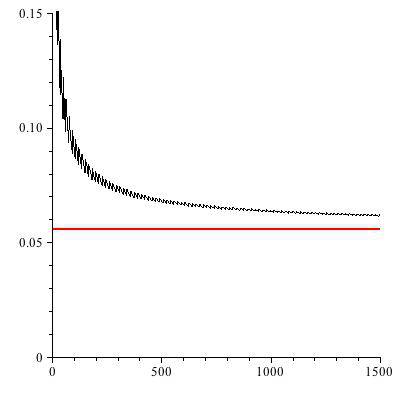
Figure 1: Comparison of $\deg(\mathsf{HS}_{n,\lceil{n/.55}\rceil})/n$ (black) with its limit (red).

Figure 1 shows the actual values of $\deg(\mathsf{HS}_{n,\lceil\alpha n\rceil})/n$ for $\alpha=1/.55$. Notice that this sequence converges rather slowly. This is due to the fact that we only take into account the first term in the asymptotic expansion of $\deg(\mathsf{HS}_{n,\lceil\alpha n\rceil})$. It would be possible to obtain the full asymptotic expansion using techniques similar to those in [4, 5]. However, this would not change the asymptotic complexity of Algorithm 1.

3.3 Complexity

We now estimate the complexity of Algorithm BooleanSolve by going through its steps and making all necessary hypotheses explicit. We consider the case when the number of variables $n$ and the number of polynomials $m$ are related by $m\sim\alpha n$ for some $\alpha\geq 1$ and $n$ is large. Also we assume that the ratio $k/n$ is controlled by a parameter $\gamma\in[0,1]$, i.e., $k=(1-\gamma)n$.

The first step (lines 4 to 6 in the algorithm) is to evaluate the polynomials $\tilde{f}_{i}$ from the polynomials $f_{i}$. With no arithmetic operations, the polynomials $f_{i}$ can first be written as polynomials in $(x_{1},\dots,x_{n-k})$ with coefficients that are polynomials of degree at most 2 in $x_{n-k+1},\dots,x_{n}$ and at most 1 in each variable. Each such coefficient has at most $1+k+\binom{k}{2}$ monomials, each of which can be evaluated with at most one arithmetic operation. The total number of these polynomial coefficients is at most $m(1+n-k+\binom{n-k}{2})$. Thus the total cost of all the evaluations of the coefficients of the polynomials $\tilde{f}_{i}$ is at most $O(n^{5}2^{(1-\gamma)n})$. This turns out to be asymptotically negligible compared to the next steps.

The next stage (line 8) of our algorithm consists in performing tests of inconsistency of the Macaulay matrices.

Proposition 8.

For any $\epsilon>0$, $\alpha\geq 1$ and sufficiently large $m=\lceil\alpha n\rceil$, the complexity of all tests of consistency of Macaulay matrices in Algorithm BooleanSolve with parameters $(m,n,k)$ is

• $O(2^{(1-\gamma+\theta F_{\alpha}(\gamma)+\epsilon)n})$ in the deterministic variant;

• of expectation $O(2^{(1-\gamma+2F_{\alpha}(\gamma)+\epsilon)n})$ in the probabilistic variant,

where $\gamma=1-k/n$, $F_{\alpha}(\gamma)=-\gamma\log_{2}(D^{D}(1-D)^{1-D})$ with $D=M(\alpha/\gamma)$, the function $M$ as in Proposition 7 and $\theta$ the complexity of linear algebra as in Proposition 2.

A notable feature of this result is that in terms of complexity, the probabilistic variant of our algorithm behaves as the deterministic one where the linear algebra would be performed in quadratic complexity (i.e., with $\theta=2$).

Proof.

We first estimate the size of the Macaulay matrices. By Proposition 7, the index $d_{0}$, which is $1+\deg(\mathsf{HS}_{n-k,m})$ behaves asymptotically like $\gamma Dn$. The function $M(x)$ is decreasing for $x\geq 1$, so that $D\leq M(1)<1/2$. Thus, $d_{0}<\gamma n/2$ for $n$ sufficiently large and Proposition 4 applies with $d=d_{0}$, $m=\lceil\alpha n\rceil$ equations and $n-k=\gamma n$ variables. For $n$ sufficiently large, the bound for $r_{\mathsf{Mac}}$ is larger than that for $c_{\mathsf{Mac}}$, since the quotient of these two bounds is ${m}/{(\frac{\gamma n}{d_{0}}-1)^{2}}$, which grows linearly with $n$.

Next, we turn to the tests of inconsistency. The previous bounds and Proposition 2 imply that the number of operations required for the computation of the row echelon form is $O(n\binom{\gamma n}{d_{0}}^{\theta})$. Similarly, by Proposition 3, the complexity of checking the consistency of each matrix by the probabilistic method is $O(r_{\mathsf{Mac}}\log(r_{\mathsf{Mac}})s_{\mathsf{Mac}})=O(n^{4}\binom{\gamma n}{d_{0}}^{2}\log{\binom{\gamma n}{d_{0}}})$ and that bound dominates the cost of the additional operations in $\mathbb{F}_{2}$. Now, Stirling’s formula implies that for any $0<b<a$, $\log\binom{an}{bn}\sim n\log(a^{a}/(b^{b}(a-b)^{a-b}))$. Setting $a=\gamma$ and $b=\gamma D$ gives the result, the extra factor being due to the exhaustive search that performs this consistency check $2^{(1-\gamma)n}$ times. ∎

In the cases where the linear system $\mathbf{u}\cdot\mathsf{M}=\mathbf{r}$ is found inconsistent, then the polynomial system itself may be consistent and the algorithm proceeds with an exhaustive search (line 9) in a system with $\gamma n$ unknowns. Each such search has cost $O(2^{(\gamma+\epsilon)n})$. As long as the number of these searches does not exceed $O(2^{(1-2\gamma+2F_{\alpha}(\gamma))n})$, the overall complexity of the algorithm is bounded by the complexity given in Proposition 8. There can be two causes for the inconsistency of the linear system that triggers such a search: the existence of an actual solution with $x_{n}=a_{n},\dots,x_{n-k+1}=a_{n-k+1}$; a witness degree of the specialized system larger than ${d}_{0}$ (e.g., if the homogenized specialized system is not boolean semi-regular). We now define a class of systems where this does not happen too much.

Definition 8.

Let $S=(f_{1},\ldots,f_{m})$ be quadratic polynomials in $\mathbb{F}_{2}[x_{1},\dots,x_{n}]$, $0\leq k=(1-\gamma)n<n$, $\alpha=m/n$ and $d_{0}=1+\deg(\mathsf{HS}_{n-k,m})$. The system $S$ is called $\gamma$-strong semi-regular if both the set of its solutions in ${\mathbb{F}_{2}^{n}}$ and the set

$$\bigl{\{}(a_{n-k+1},\dots,a_{n})\in\mathbb{F}_{2}^{k}\mid\\ \operatorname{d_{wit}}(f_{1}(x_{1},\dots,x_{n-k},a_{n-k+1},\dots,a_{n}),\dots,f_{m}(x_{1},\dots,x_{n-k},a_{n-k+1},\dots,a_{n}))>d_{0}\bigr{\}}$$

have cardinality at most ${2^{(1-2\gamma+2F_{\alpha}(\gamma))n}}$, with $F_{\alpha}$ as in Proposition 8.

Note that since $1-2\gamma+2F_{\alpha}(\gamma)$ is a decreasing function of $\gamma$, a $\gamma$-strong semi-regular system is also $\gamma^{\prime}$-strong semi-regular for any $\gamma^{\prime}<\gamma$.

The first condition for a system to be $\gamma$-strong semi-regular concerns its number of solutions. For boolean systems drawn uniformly at random, it is known that the probability that the number of boolean solutions is $s$ decreases more than exponentially with $s$ [24], so that the first condition is fulfilled with large probability. The second condition is related to the proportion of boolean semi-regular systems. We discuss this condition in the next section and show that it is also of large probability experimentally. Under this assumption of $\gamma$-strong semi-regularity, we now state the complexity of the algorithm obtained by optimizing the choice of the number $k$ of variables that are specialized.

We first discuss large values of $\gamma$. The function $1-2\gamma+2F_{\alpha}(\gamma)$ is decreasing with $\alpha$ and negative when $\gamma=1$. Thus, the first condition implies that a $1$-strong semi-regular system has no solution. By continuity, this behavior persists for $\gamma$ close to 1 and actually holds for $\gamma\in(0.824,1)$. It also persists for smaller values of $\gamma$ and larger $\alpha$.

Corollary 2.

With the same notations as in Prop. 8, when a system is $\gamma$-strong semi-regular with $\alpha$ and $\gamma$ such that $1-2\gamma+2F_{\alpha}(\gamma)<0$, then it is inconsistent and detected by Algorithm BooleanSolve with parameters $(m,n,0)$ in $O(2^{(\theta F_{\alpha}(1)+\epsilon)n})$ operations.

Figure 2: Exponent of the complexity for inconsistent systems in terms of the ratio $\alpha$ (see Thm. 2 and Cor. 2)

The value of the exponent $\theta F_{\alpha}(1)$ in terms of $\alpha$ is plotted in Figure 2 (it corresponds to the right part of the plots, i.e. $\alpha>1.82$ for $\theta=2$, $\alpha>2.48$ for $\theta=2.376$, $\alpha>3.64$ for $\theta=3$).

Proof.

The hypothesis implies that the system has no solution and that its witness degree is bounded by $d_{0}$, so that its absence of solution is detected by the linear algebra step in degree $d_{0}$. In that case, no exhaustive search is needed. ∎

For smaller values of $\gamma$, the algorithm requires exhaustive searches. The optimal choice of $k$ is obtained by an optimization on the complexity estimate. This leads to the following complexity estimates. In the next section, we argue that the required strong semi-regularities are very likely in practice, so that the only choice left to the user is that of the linear algebra routine.

Theorem 2.

Let $S=(f_{1},\dots,f_{m})$ be a system of quadratic polynomials in $\mathbb{F}_{2}[x_{1},\dots,x_{n}]$, with $m=\lceil\alpha n\rceil$ and $\alpha\geq 1$. Then Algorithm BooleanSolve finds all its roots in $\mathbb{F}_{2}^{n}$ with a number of arithmetic operations in $\mathbb{F}_{2}$ that is

• $O(2^{(1-0.112\alpha)n})$ if $S$ is $(.27\alpha)$-strong semi-regular using Gaussian elimination for the linear algebra step;

• $O(2^{(1-0.159\alpha)n})$ if $S$ is $(.40\alpha)$-strong semi-regular using computation of the row echelon form with Coppersmith-Winograd multiplication;

• of expectation $O(2^{(1-0.208\alpha)n})$ if $S$ is $(.55\alpha)$-strong semi-regular using the probabilistic Algorithm 2.

In all cases, the value of $k$ passed to the algorithm is $\lceil n(1-\gamma)\rceil$ with $\gamma$ corresponding to the strong semi-regularity.

Proof.

The correctness of the algorithm has already been proved in Proposition 1. Only the complexity remains to be proved.

By definition of strong semi-regularity, the number of exhaustive searches that need be performed in line 9 of the Algorithm is $O(2^{(1-2\gamma+2F_{\alpha}(\gamma))n})$, each of them using $O(2^{(\gamma+\epsilon)n})$ arithmetic operations for any $\epsilon>0$. It follows that the overall cost of these exhaustive searches is $O(2^{(1-\gamma+2F_{\alpha}(\gamma)+\epsilon)n})$; it is bounded by the cost of the tests of inconsistency. We now choose $\gamma$ in such a way as to minimize this cost, in terms of $\alpha$. Direct computations lead to the following numerical results, that conclude the proof. ∎

Lemma 2.

With the same notation as in Proposition 8, the function $1-\gamma+\theta F_{\alpha}(\gamma)$ is bounded by

• $1-0.112\alpha$ when $\theta=3$ and $\gamma=0.27\alpha$;

• $1-0.159\alpha$ when $\theta=2.376$ and $\gamma=0.40\alpha$;

• $1-0.208\alpha$ when $\theta=2$ and $\gamma=0.55\alpha$.

Proof.

The function $1-\gamma+\theta F_{\alpha}(\gamma)$ has two parameters but its extrema can be found by reducing it to a one parameter function. Indeed, this function is maximal for $\alpha\geq 1$ and $\gamma\in[0,1]$ when $(-\gamma+\theta F_{\alpha}(\gamma))/\alpha$ is. Setting $\lambda=\gamma/\alpha$, this is exactly $-\lambda+\theta F_{1}(\lambda)$, with $\lambda\in[0,1/\alpha]$. Direct computations lead to the optimal $\lambda$’s: $\lambda=\min(1/\alpha,0.27)$ when $\theta=3$, $\lambda=\min(1/\alpha,0.40)$ when $\theta=2.376$, $\lambda=\min(1/\alpha,0.55)$ when $\theta=2$. ∎

4 Numerical Experiments on Random Systems

Probabilistic model. In this section, we study experimentally the behavior of Algorithm BooleanSolve of random quadratic systems where each coefficient is 0 or 1 with probability 1/2. These random boolean quadratic systems appear naturally in Cryptology since the security of several recent cryptosystems relies directly on the difficulty of solving such systems (see e.g., [6, 7]).

4.1 $\gamma$-strong semi-regularity

The goal of this section is to give experimental evidence that the assumption of $\gamma$-strong semi-regularity is not a strong condition for random boolean systems. This is related to the notoriously difficult conjecture by [23], which states that in characteristic $0$, almost all systems are semi-regular (with the meaning of semi-regularity given in [5]), see also [31].

Consequently, we propose the following conjecture, which can be seen as a variant of Fröberg’s conjecture for boolean systems:

Conjecture 1.

For any $\alpha\geq 1$ and $\gamma<1$ such that $1-2\gamma+2F_{\alpha}(\gamma)>0$, the proportion of $\gamma$-strong semi-regular systems of $\lceil\alpha n\rceil$ quadratic polynomials in $\mathbb{F}_{2}[x_{1},\dots,x_{n}]$ tends to 1 when $n\rightarrow\infty$.

The rest of this section is devoted to providing experiments supporting this conjecture.

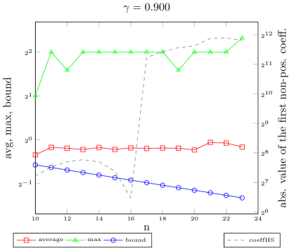
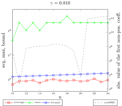
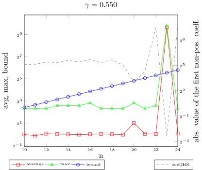
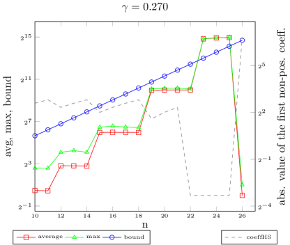
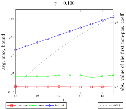
Figure 3: Relation between the quality of the filtering, the value of the first nonpositive coefficient of $\mathsf{HS}_{\lfloor\gamma n\rfloor,n}$, and $\gamma$-strong semi-regularity. In red (resp. green), the average (resp. maximum) number of specializations for which the linear system is inconsistent. In blue, the bound for $\gamma$-strong regularity. Dashed line: absolute value of the first non positive coefficient of $\mathsf{HS}_{\lfloor\gamma n\rfloor,n}$.

In Figure 3, we show the relation between the value of the first nonpositive coefficient of the power series expansion of $\mathsf{HS}_{\lfloor\gamma n\rfloor,n}$ and $\gamma$-strong semi-regularity for small values of $n=m$ (i.e. $\alpha=1$). For each $n$, the experiments are conducted on 1000 random quadratic boolean systems. For each of these systems, we compute the $2^{\lceil(1-\gamma)n\rceil}$ specialized systems and we count the number of specializations for which the filtering linear system is inconsistent.

Four curves are represented on each chart in Figure 3. The red (resp. green) one represents the average (resp. maximal) number of specializations for which the linear system (step 8 of Algorithm BooleanSolve) is inconsistent. In contrast, the blue curve shows the upper bound on this number of specializations required to be $\gamma$-strong semi-regular (see Definition 8). The black curve shows the absolute value of the first nonpositive coefficient of the corresponding power series (i.e. $\mathsf{HS}_{\lfloor\gamma n\rfloor,n}$). The $y$-axis is represented in logarithmic scale. The value $\gamma=0.1$ is never used in the complexity analysis (since in Theorem 2, $\gamma\geq.27$ for any value of $\alpha\geq 1$). However, it is still interesting to study the behavior of Algorithm 1 when almost all variables are specialized: the filtering remains very efficient in this case, and the branches which are explored during the second stage of the exhaustive search correspond to those containing solutions of the system.

Interpretation of Figure 3. First, notice that for $\gamma\leq 0.55$ the green curve is always below the blue one (except for the case $\gamma=.55,n=23$), meaning that during our experiments, all randomly generated systems with those parameters were $\gamma$-strong semi-regular.

Next, in most curves (except $\gamma=0.27$), the average (resp. maximal) number of points where the specialization leads to an inconsistent linear system is close to $1$ (resp. $5$). This can be explained by a simple Poisson model. Indeed, the number of solutions of a random boolean system with as many equations as unknowns follows a Poisson law with parameter $1$ (see [24]). Therefore, the expectation of the number of solutions is $1$. The expectation of the maximum of the number of solutions of $1000$ random systems is then given as the maximum of 1000 iid random variables $P_{1},\ldots,P_{1000}$ following a Poisson law of parameter $1$:

$$\mathbf{E}(\max(P_{1},\ldots,P_{1000}))=\sum_{k\geq 1}{k\left((e^{-1}\sum_{i=0}^{k}{\frac{1}{i!}})^{1000}-(e^{-1}\sum_{i=0}^{k-1}{\frac{1}{i!}})^{1000}\right)}\simeq 5.51,$$

which explains very well the observed behaviour.

This means that during Algorithm 1 with these parameters, almost all specializations giving rise to an inconsistent system correspond to a branch of the exhaustive search which contains an actual solution of the system. Therefore, the filtering is very efficient for those parameters.

Few specializations. In the case $\gamma=0.9$, the blue curve has a negative slope. This is due to the fact that the quantity $1-2\gamma+2F_{\alpha}(\gamma)$ (see Definition 8) is negative for $\alpha=1$ and $\gamma>0.82308$. Therefore, we cannot expect that a large proportion of boolean systems are $\gamma$-strong semi-regular in this setting. A limit case is investigated in the chart corresponding to $\gamma=0.81$. There, $1-2\gamma+2F_{\alpha}(\gamma)\approx 0.0102$ is positive but very close to zero. Experiments show that random boolean systems with these parameters and $10\leq n\leq 24$ are $\gamma$-strong semi-regular with probability approximately equal to $0.75$.

Absolute value of the first nonpositive coefficient of $\mathsf{HS}_{\lfloor\gamma n\rfloor,n}$ and $\gamma$-strong semi-regularity. Another interesting setting is $\gamma=.55,n=23$. Here, no generated systems were $\gamma$-strong semi-regular (although all generated systems for $n\neq 23$ were $\gamma$-strong semi-regular). As explained in Section 5.1, this is due to the fact that the first nonpositive coefficient of the power series expansion of $\mathsf{HS}_{\lfloor\gamma n\rfloor,n}$ is equal to zero. In Section 5.2, we show that this phenomenon can be avoided by a simple variant of the algorithm.

A similar phenomenon happens for $\gamma=.27$: the first nonpositive coefficient of the power series has small absolute value. It is an accident due to the fact that this coefficient is close to zero for $n\leq 25$ (see Figure 4). On this chart, we can see clearly the relation between the absolute value of the first nonpositive coefficient of $\mathsf{HS}_{\lfloor\gamma n\rfloor,n}$ and the number of specializations for which the consistency test fails.

Indeed, experiments on $1000$ random systems with $\gamma=.27$ and $n=26$ were conducted and in this case the average number of specializations for which the linear system is inconsistent is $1$.

These experiments justify the fact that the complexity analysis conducted in Section 3 is relevant for a large class of boolean systems. Also, it shows that the random systems for which the filtering may not be efficient can be detected a priori by looking at the absolute value of the first nonpositive coefficient in the power series. If this value is small, we show in Section 5.2 that the quality of the filtering can be improved at low cost by adding redundancy.

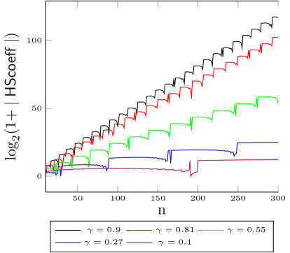
Figure 4: Evolution of the logarithm of the absolute value of the first nonpositive coefficient of $\mathsf{HS}_{\lfloor\gamma n\rfloor,n}$.

Figure 4 shows the evolution of the logarithm of the absolute value of the first nonpositive coefficient of $\mathsf{HS}_{\lfloor\gamma n\rfloor,n}$. This absolute value seems to grow exponentially with $n$ for any given $\gamma$. Since the quality of the filtering is related to this absolute value, these experiments suggest that the proportion of $\gamma$-strong semi-regular systems tends towards 1 when $n$ grows, as formulated in Conjecture 1.

4.2 Numerical estimates of the complexity

When $n=m$ and in the most favorable algorithmic case, our complexity estimate uses $\gamma=.55$. For this value, we display in Figure 1 (page 1) a comparison of the behaviour of $\deg(\mathsf{HS}_{n,\lceil{\frac{n}{\gamma}}\rceil})/n$ and its limit. This picture shows a relatively slow convergence. Thus, for a given number $n$ of variables it is more interesting to optimize $\gamma$ using the exact value of $\deg(\mathsf{HS}_{\lfloor{\gamma n}\rfloor,n})$ rather than a first order asymptotic estimate. In the same spirit, one can also use the actual values given by Eq. (2) for the Macaulay matrix. Thus we seek to find $\gamma$ that minimizes the following bounds on the number of operations:

$$\begin{array}[]{l}2^{(1-\gamma)n}r_{\mathsf{Mac}}c_{\mathsf{Mac}}\min(r_{\mathsf{Mac}},c_{\mathsf{Mac}})^{\theta-2},\\ \text{resp.}\quad 2^{(1-\gamma)n}\max(r_{\mathsf{Mac}},c_{\mathsf{Mac}})\log\max(r_{\mathsf{Mac}},c_{\mathsf{Mac}})s_{\mathsf{Mac}}\end{array}$$ (10)

in the deterministic (resp. probabilistic) variants, using Eq. (3) with $n$ equations, $\lfloor{\gamma n}\rfloor$ variables and $d=\deg(\mathsf{HS}_{\lfloor{\gamma n}\rfloor,n})$. The corresponding values of $\gamma$ are given in Figure 5, together with the corresponding values of the quantities in Eq. (10). Although these values do not take into account the constants hidden in the $O()$ estimates of the complexity, they suggest the relevance of these algorithms in the cryptographic sizes: the threshold between exhaustive search and our algorithm with Gaussian elimination is $n\simeq 280$, while the asymptotically faster Las Vegas variant starts being faster than exhaustive search for $n$ larger than 200 and beats deterministic Gaussian elimination for $n$ larger than 160.

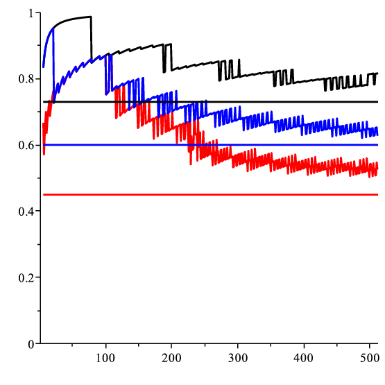
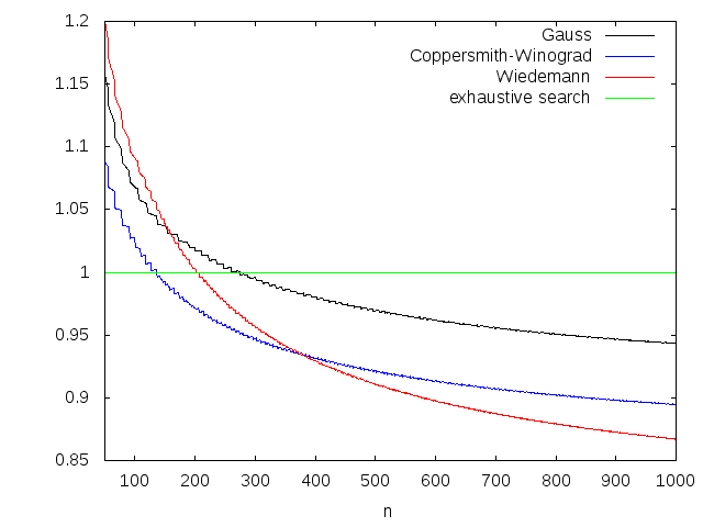
Figure 5: Left: optimal values of $\gamma$ for the probabilistic variant (red), the deterministic variant with Gaussian elimination (black) and Coppersmith-Winograd matrix multiplication (blue), and their limits. Right: corresponding values of $\log_{2}N/n$, with $N$ given by (10). The green line corresponds to an exhaustive search.

5 Extensions and Applications

5.1 Adding Redundancy to Avoid Rank Defects

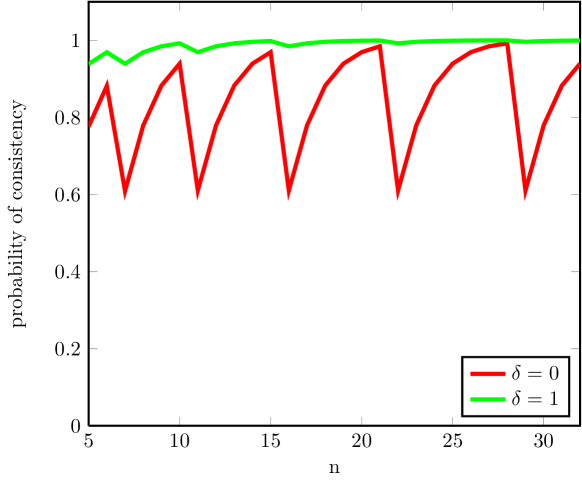
Figure 6: Proportion of specialized quadratic systems for which the linear system (line 9 of Algorithm 1) is consistent. Parameters: $k=\left\lceil 1/2+n-\frac{\sqrt{-7+8n}}{2}\right\rceil$. In red, $\delta=0$ (corresponding to Algorithm 1); in green, $\delta=1$ (see Algorithm 3 of Section 5.2).

We showed in Section 4.1 that when the first nonpositive coefficient of $\mathsf{HS}_{n-k,n}$ is close to zero, then the linear filtering may not be as efficient as expected (for instance in the case $\gamma=.55$, $n=23$ in Figure 3). Another case is shown in Figure 6. The curve $\delta=0$ shows the behavior of Algorithm 1 on random square systems ($m=n$) where $k$ is chosen as small as possible such that the witness degree is $\operatorname{d_{wit}}=2$: this is obtained by choosing $k=\left\lceil 1/2+n-\frac{\sqrt{-7+8n}}{2}\right\rceil$ (that is $d_{0}=2$).

First, we observe that specializing a uniformly distributed random quadratic polynomial $P\in\mathbb{F}_{2}[x_{1},\ldots,x_{n}]$ at a uniformly distributed random point in $\mathbb{F}_{2}^{k}$ yields a random polynomial that is also uniformly distributed in $\mathbb{F}_{2}[x_{1},\ldots,x_{n-k}]$. We assume here that $P$ is reduced modulo the field equations $\langle x_{1}^{2}-x_{1},\ldots,x_{n}^{2}-x_{n}\rangle$. Let us assume first that $k=1$. Then $P$ can be rewritten as

$$P(x_{1},\ldots,x_{n})=x_{n}P_{1}(x_{1},\ldots,x_{n-1})+P_{2}(x_{1},\ldots,x_{n-1}),$$

where $P_{1}$ (resp. $P_{2}$) is a random polynomial following a uniform distribution on the set of reduced boolean polynomials of degree $1$ (resp. of degree $2$) in $\mathbb{F}_{2}[x_{1},\ldots,x_{n-1}]$. Therefore, if $a\in\mathbb{F}_{2}$ is a random variable, $P(x_{1},\ldots,x_{n-1},a)\in\mathbb{F}_{2}[x_{1},\ldots,x_{n-1}]$ is either $P_{1}$ or $P_{1}+P_{2}$ and thus follows a uniform distribution on the set of reduced quadratic boolean polynomials. The extension to arbitrary $k<n$ follows by induction.

Consequently, in the special case $d_{0}=2$ of Figure 6 the boolean Macaulay matrix of a specialized system will be uniformly distributed among the boolean matrices with the same dimensions. Also, due to the choice of $k$, it will be roughly square. However, in $\mathbb{F}_{2}$, the probability that a random square matrix has full rank is not close to $1$. An estimate of this probability can be obtained as follows.

The probability that a random $p\times q$ boolean matrix has rank $r$ is (see [21, 35])

$$P(p,q,r)=2^{-pq}\displaystyle\frac{\prod_{j=0}^{r-1}(2^{p}-2^{j})\prod_{j=0}^{r-1}(2^{q}-2^{j})}{\prod_{j=0}^{r-1}(2^{r}-2^{j})}.$$

Therefore, given a nonzero vector $\mathbf{v}\in\mathbb{F}_{2}^{p}$ and a random boolean $p\times q$ matrix $\mathsf{M}$, the probability that the linear system $\mathbf{u}\cdot\mathsf{M}=\mathbf{v}$ is consistent is

$$Q(p,q)=\sum_{i=1}^{p}P(p,q,i)\left(\frac{2^{i}-1}{2^{q}-1}\right).$$

Direct numerical computations show that for square matrices, $Q(p,p)\approx 0.61$ as soon as $p\geq 4$. This probability corresponds to the valleys of the curve $\delta=0$ in Figure 6. Also, it can be noticed that $Q(p,q)$ grows quickly with $p-q$. For instance, $Q(p+6,p)\approx 0.99$ when $p\geq 1$.

Consequently, it is interesting to specialize more variables than $k$ in some cases (especially when the first nonpositive coefficient of ${(1+t)^{n-k}}/({(1-t)(1+t^{2})^{m}})$ has small absolute value): doing so increases the difference between the dimensions of the Macaulay matrices. This does not change the correctness of the algorithm (nor its asymptotic complexity), but increases the effectiveness of the filtering performed by linear algebra.

5.2 Improving the quality of the filtering for small values of $n$

In this section, we propose an extension of Algorithm BooleanSolve which takes an extra argument $\delta$, in order to avoid the behavior of the algorithm shown in Section 5.1. The main idea is to specialize $k+\delta$ variables, but to take only $k$ into account for the computation of $d_{0}$. Consequently, the difference between the number of columns and the rank of the Macaulay matrix is not too small, and hence the linear filtering performs better. The resulting algorithm is given in Algorithm 3.

Algorithm 3 improved BooleanSolve.

1:$m,n,k,\delta\in\mathbb{N}$ such that $k+\delta<n\leq m$ and $f_{1},\ldots,f_{m}$ quadratic polynomials in $\mathbb{F}_{2}[x_{1},\ldots,x_{n}]$.

2:The set of boolean solutions of the system $f_{1}=\dots=f_{m}=0$.

3:$S:=\emptyset$.

4:${d_{0}}:=$ index of the first nonpositive coefficient in the series expansion of the rational function $\frac{(1+t)^{n-k}}{(1-t)(1+t^{2})^{m}}$.

5:for all $(a_{n-k-\delta+1},\ldots,a_{n})\in\mathbb{F}_{2}^{k+\delta}$ do

6:     for $i$ from $1$ to $m$ do

7:         $\tilde{f}_{i}(x_{1},\ldots,x_{n-k-\delta}):=f_{i}(x_{1},\ldots,x_{n-k-\delta},a_{n-k-\delta+1},\ldots,a_{n})$.

8:     end for

9:     $\mathsf{M}:=$ boolean Macaulay matrix of $(\tilde{f}_{1},\ldots,\tilde{f}_{m})$ in degree ${d_{0}}$.

10:     if the system $\mathbf{u}\cdot\mathsf{M}=\mathbf{r}$ is inconsistent then$\triangleright$ $\mathbf{r}$ as defined in Lemma 1

11:         $T:=$ solutions of the system ($\tilde{f}_{1}=\cdots=\tilde{f}_{m}=0$) (exhaustive search).

12:         for all $(t_{1},\ldots,t_{n-k-\delta})\in T$ do

13:              $S:=S\cup\{(t_{1},\ldots,t_{n-k-\delta},a_{n-k-\delta+1},\ldots,a_{n})\}$.

14:         end for

15:     end if

16:end for

17:return $S$.

In Figure 6, we show the role of the parameter $\delta$ when $k$ is chosen minimal such that $d_{0}=2$: adding redundancy by choosing a nonzero $\delta$ can greatly improve the quality of the filtering (in practice, choosing $\delta=1$ is sufficient).

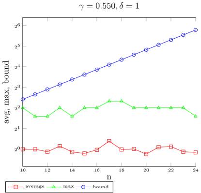
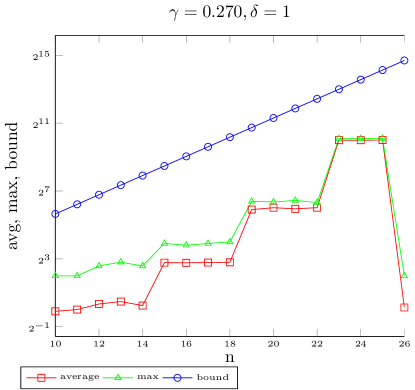
Figure 7: Quality of the filtering with $\delta=1$.

Figure 7 shows further experimental evidence that adding redundancy by choosing $\delta=1$ permits to avoid problems occurring when the first nonpositive coefficient of $\mathsf{HS}_{n-k,m}$ is close to zero. For instance, the peak at $\gamma=.55$, $n=23$ that appeared in Figure 3 disappears when $\delta=1$.

5.3 Cases with Low Degree of Regularity

In some cases, when the boolean system is not random, the choice of $d_{0}$ proposed in Algorithm BooleanSolve may be too large. This happens for instance for systems that have inner structure, which has an impact on the algebraic structure of the ideal generated by the polynomials. Examples of such structure can be found in Cryptology, for instance with boolean systems coming for the HFE cryptosystem [32], as shown in [19].

For these systems, the choice of $d_{0}$ as the index of the first non-positive coefficient of $\mathsf{HS}_{n,m}$ would be very pessimistic, since the Macaulay matrices in degree $d_{0}$ would be larger than necessary. However, if estimates of the witness degree are known (this is the case for HFE), then $d_{0}$ can be chosen accordingly as a parameter of the Algorithm BooleanSolve.

5.4 Application in Cryptology

Careful implementation of the algorithm will be necessary to estimate accurately the efficiency of the BooleanSolve algorithm. For instance a crucial operation is the Wiedemann (or block Wiedemann) algorithm; in practice, it is probably useless to work in a field extension $\mathbb{F}_{2^{k}}$ as requested by Proposition 3. Working directly over $\mathbb{F}_{2}$ and packing several elements (bits) into words may have a dramatic effect on the constant hidden in Theorem 2. In the following we estimate the impact of the new algorithm from the point of view of a user in Cryptology. In other words, if the security of a cryptosystem relies on the hardness of solving a polynomial system, by how much must the parameters be increased to keep the same level of security?

The stream cipher QUAD [6, 7] enjoys a provable security argument to support its conjectured strength. It relies on the iteration of a set of overdetermined multivariate quadratic polynomials over $\mathbb{F}_{2}$ so that the security of the keystream generation is related, in the concrete security model, to the difficulty of solving the Boolean MQ SAT problem. A theoretical bound is used in [7] to obtain secure parameters for a given security bound $T$ and a given maximal length $L$ of the keystream sequence that can be generated with a pair (key, IV): for instance (see [7] p. 1711), for $T=2^{80},L=2^{40},k=2$ and an advantage of more than $\varepsilon=1/100$, the bound gives $n\geq 331$. We report in the following table various values of $n$ depending on $L$, $T$ and $\varepsilon$:

T	L	$\varepsilon$	n
$2^{80}$	$2^{40}$	1/100	331
$2^{80}$	$2^{22}$	1/100	253
$2^{160}$	$2^{80}$	1/100	613
$2^{160}$	$2^{40}$	1/100	445
$2^{160}$	$2^{40}$	1/1000	448
$2^{160}$	$2^{40}$	1/10000	467
$2^{256}$	$2^{40}$	1/100	584
$2^{256}$	$2^{80}$	1/100	758

Security parameters for the stream cipher QUAD [7]

Now, the question is to achieve a security bound for $T=2^{256}$; what are the minimal values of $m$ and $n$ ensuring that solving the Boolean MQ SAT requires at least $T$ bit-operations? Using the complexity analysis of the BooleanSolve algorithm we can derive useful lower bounds for $n$ when $m=n$ or $m=2\,n$ ($m=2\,n$ corresponds to the recommended parameters for QUAD). In the following table we report the corresponding values:

Security Bound $T$	$2^{128}$	$2^{256}$	$2^{512}$	$2^{1024}$
Minimal value of $n$ when $m=n$	$128$	$270$	$576$	1202
Minimal value of $n$ when $m=2\,n$	$145$	$335$	$738$	1580

Comparing with exhaustive search we can see from this table that:

• our algorithm does not improve upon exhaustive search when $n$ is small (for instance when $m=n$ and $T=2^{128}$ that are the recommended parameters);

• by contrast, our algorithm can take advantage of the overdeterminedness of the algebraic systems: this explains why the values we recommend are larger than expected when $n$ is large and/or $m/n>1$.

Acknowledgments

We wish to thank D. Bernstein, C. Diem, E. Kaltofen and L. Perret for valuable comments and pointers to important references. This work was supported in part by the Microsoft Research-INRIA Joint Centre and by the CAC grant (ANR-09-JCJCJ-0064-01) and the HPAC grant of the French National Research Agency.

References

- [1] M. Albrecht, J.-C. Faugère, P. Farshim, and L. Perret. Polly cracker, revisited. In Advances in Cryptology – Asiacrypt 2011, volume 7073 of Lecture Notes in Computer Science, pages 1–14. Springer-Verlag, 2011.
- [2] G. Ars, J.-C. Faugère, H. Imai, M. Kawazoe, and M. Sugita. Comparison between XL and Gröbner basis algorithms. In Advances in Cryptology – AsiaCrypt 2004, volume 3329 of Lecture Notes in Computer Science, pages 157–167, 2004.
- [3] M. Bardet. Étude des Systèmes Algébriques Surdéterminés. Applications aux Codes et à la Cryptographie. PhD thesis, Université Paris 6, 2004.
- [4] M. Bardet, J.-C. Faugère, and B. Salvy. On the complexity of Gröbner basis computation of semi-regular overdetermined algebraic equations. In Proceedings of the International Conference on Polynomial System Solving (ISCPP), pages 71–74, 2004.
- [5] M. Bardet, J.-C. Faugère, B. Salvy, and B.-Y. Yang. Asymptotic expansion of the degree of regularity for semi-regular systems of equations. In Effective Methods in Algebraic Geometry (MEGA), pages 1–14, 2005.
- [6] C. Berbain, H. Gilbert, and J. Patarin. QUAD: A practical stream cipher with provable security. In S. Vaudenay, editor, Advances in Cryptology - Eurocrypt 2006, volume 4004 of Lecture Notes in Computer Science, pages 109–128. Springer, 2006.
- [7] C. Berbain, H. Gilbert, and J. Patarin. QUAD: A multivariate stream cipher with provable security. Journal of Symbolic Computation, 44:1703–1723, 2009.
- [8] L. Bettale, J.-C. Faugère, and L. Perret. Hybrid approach for solving multivariate systems over finite fields. Journal of Mathematical Cryptology, 3:177–197, 2009.
- [9] L. Bettale, J.-C. Faugère, and L. Perret. Solving polynomial systems over finite fields: Improved analysis of the hybrid approach. In ISSAC’12: Proceedings of the 2012 International Symposium on Symbolic and Algebraic Computation, pages 1–12, 2012.
- [10] C. Bouillaguet, H.-C. Chen, C.-M. Cheng, T. Chou, R. Niederhagen, B.-Y. Yang, and A. Shamir. Fast exhaustive search for polynomial systems in . In Cryptographic Hardware and Embedded Systems, CHES 2010, volume 6225 of Lecture Notes in Computer Science, pages 203–218, 2010.
- [11] B. Buchberger. An algorithm for finding the basis elements of the residue class ring of a zero dimensional polynomial ideal. PhD thesis, University of Innsbruck, 1965.
- [12] J. F. Canny, E. Kaltofen, and L. Yagati. Solving systems of nonlinear polynomial equations faster. In ISSAC’89: Proceedings of the 1989 International Symposium on Symbolic and Algebraic Computation, pages 121–128. ACM Press, 1989.
- [13] D. Coppersmith and S. Winograd. Matrix multiplication via arithmetic progressions. Journal of Symbolic Computation, 9(3):251–280, 1990.
- [14] D. Cox, J. Little, and D. O’Shea. Ideals, Varieties and Algorithms. Springer, 3rd edition, 1997.
- [15] D. Eisenbud. Commutative Algebra with a View Toward Algebraic Geometry. Springer, 1995.
- [16] J.-C. Faugère. A new efficient algorithm for computing Gröbner bases (F4). Journal of Pure and Applied Algebra, 139(1–3):61–88, 1999.
- [17] J.-C. Faugère. A new efficient algorithm for computing Gröbner bases without reductions to zero (F5). In T. Mora, editor, ISSAC’02: Proceedings of the 2002 International Symposium on Symbolic and Algebraic Computation, pages 75–83. ACM Press, 2002.
- [18] J.-C. Faugère, P. Gianni, D. Lazard, and T. Mora. Efficient computation of zero-dimensional Gröbner bases by change of ordering. Journal of Symbolic Computation, 16(4):329–344, 1993.
- [19] J.-C. Faugère and A. Joux. Algebraic cryptanalysis of Hidden Field Equation (HFE) cryptosystems using Gröbner bases. In Advances in Cryptology – Crypto 2003, volume 2729 of Lecture Notes in Computer Science, pages 44–60. Springer, 2003.
- [20] J.-C. Faugère, A. Otmani, L. Perret, and J.-P. Tillich. Algebraic cryptanalysis of McEliece variants with compact keys. In Advances in Cryptology – Eurocrypt 2010, volume 6110 of Lecture Notes in Computer Science, pages 279–298. Springer Verlag, 2010.
- [21] S. D. Fisher and M. N. Alexander. Matrices over a finite field. The American Mathematical Monthly, 73(6):639–641, 1966.
- [22] A. S. Fraenkel and Y. Yesha. Complexity of problems in games, graphs and algebraic equations. Discrete Applied Mathematics, 1(1-2):15–30, 1979.
- [23] R. Fröberg. An inequality for Hilbert series of graded algebras. Mathematica Scandinavica, 56:117–144, 1985.
- [24] G. Fusco and E. Bach. Phase transition of multivariate polynomial systems. In Theory and Applications of Models of Computation (TAMC), volume 4484 of Lecture Notes in Computer Science, pages 632–645, 2007.
- [25] M. Giesbrecht, A. Lobo, and B. D. Saunders. Certifying inconsistency of sparse linear systems. In ISSAC’98: Proceedings of the 1998 International Symposium on Symbolic and Algebraic Computation, pages 113–119. ACM Press, 1998.
- [26] Z. Jelonek. On the effective Nullstellensatz. Inventiones Mathematicae, 162(1):1–17, 2005.
- [27] E. Kaltofen and B. D. Saunders. On Wiedemann’s method of solving sparse linear systems. In Applied Algebra, Algebraic Algorithms and Error-Correcting Codes, volume 539 of Lecture Notes in Computer Science, pages 29–38. Springer, 1991.
- [28] A. Kipnis, J. Patarin, and L. Goubin. Unbalanced oil and vinegar signature schemes. In Advances in Cryptology – Eurocrypt’99, volume 1592 of Lecture Notes in Computer Science, pages 206–222, 1999.
- [29] A. Kipnis and A. Shamir. Cryptanalysis of the HFE public key cryptosystem by relinearization. In Advances in Cryptology – Crypto’99, volume 1666 of Lecture Notes in Computer Science, pages 19–30. Springer, 1999.
- [30] F. S. Macaulay. On some formulæ in elimination. Proceedings of the London Mathematical Society, 33(1):3–27, 1902.
- [31] G. Moreno-Socías. Degrevlex Gröbner bases of generic complete intersections. Journal of Pure and Applied Algebra, 180(3):263–283, 2003.
- [32] J. Patarin. Hidden Fields Equations (HFE) and Isomorphisms of Polynomials (IP): Two new families of asymmetric algorithms. In Advances in Cryptology – Eurocrypt’96, volume 1070 of Lecture Notes in Computer Science, pages 33–48. Springer, 1996.
- [33] I. Semaev. On solving sparse algebraic equations over finite fields. Design, Codes and Cryptography, 49(1-3):47–60, 2008.
- [34] I. Semaev. Sparse algebraic equations over finite fields. SIAM Journal on Computing, 39(2):388–409, 2009.
- [35] E. L. Stitzinger. The probability that a linear system is consistent. Linear and Multilinear Algebra, 21(4):367–371, 1987.
- [36] A. Storjohann. Algorithms for Matrix Canonical Forms. PhD thesis, Department of Computer Science, ETH, Zürich, 2000.
- [37] A. Stothers. On the Complexity of Matrix Multiplication. PhD thesis, University of Edinburgh, 2010.
- [38] V. Vassilevska Williams. Breaking the Coppersmith-Winograd barrier. Technical report, 2011.
- [39] G. Villard. Further analysis of Coppersmith’s block Wiedemann algorithm for the solution of sparse linear systems. In ISSAC’97: Proceedings of the 1997 International Symposium on Symbolic and Algebraic Computation, pages 32–39. ACM Press, 1997.
- [40] D. Wiedemann. Solving sparse linear equations over finite fields. IEEE Transactions on Information Theory, 32(1):54–62, 1986.
- [41] B.-Y. Yang and J.-M. Chen. Theoretical analysis of XL over small fields. In Information Security and Privacy 2004, volume 3108 of Lecture Notes in Computer Science, pages 277–288, 2004.
- [42] B.-Y. Yang, J.-M. Chen, and N. T. Courtois. On asymptotic security estimates in XL and Gröbner bases-related algebraic cryptanalysis. In ICICS 2004, volume 3269 of Lecture Notes in Computer Science, pages 401–413. Springer-Verlag, 2004.