Flavor of quiver-like realizations of effective supersymmetry

Roberto Auzzi, Amit Giveon and Sven Bjarke Gudnason

Racah Institute of Physics, The Hebrew University, Jerusalem, 91904, Israel

Abstract

We present a class of supersymmetric models which address the flavor puzzle and have an inverted hierarchy of sfermions. Their construction involves quiver-like models with link fields in generic representations. The magnitude of Standard-Model parameters is obtained naturally and a relatively heavy Higgs boson is allowed without fine tuning. Collider signatures of such models are possibly within the reach of LHC in the near future.

 
auzzi(at)phys.huji.ac.il
giveon(at)phys.huji.ac.il
gudnason(at)phys.huji.ac.il

1 Introduction

It is now an exciting period for supersymmetry (SUSY), as the LHC is closing in on simplified SUSY models pointing theorists towards certain parts of parameter space. As the experimental limits are getting exceedingly harder for gauge mediated SUSY-breaking models which are flavor blind (see [1] for a summary of current collider constraints), one possibility [2, 3] that is being extensively explored now is “effective supersymmetry.” This “more Minimal Supersymmetric Standard Model (MSSM)” is supersymmetric in the UV but may differ significantly from the MSSM; near the weak scale it necessarily includes just the particles required for naturalness. Hence, this type of models often possess an inverted hierarchy of sparticle masses, i.e. the stop being relatively light while the sup and scharm may be considerably heavier (and similarly for the down-type squarks); see e.g. [4, 5, 6, 7, 8, 9].

In addition to being motivated by current trends in collider limits, the models of inverted hierarchy might be related to one of the biggest and yet unsolved puzzles of particle physics, viz. the flavor problem. The first level of difficulty lies in providing an explanation to the SM fermion mass hierarchy and the CKM matrix. The second level of trouble is due to the mixing of squarks, generically giving rise to flavor changing neutral currents (FCNCs). Several ways of addressing the flavor puzzle have been put forward in the literature. One of them involves horizontal symmetries which suppress some of the Yukawa couplings [10] and in turn FCNCs. Another possibility is having a strongly coupled conformal sector which provides large anomalous dimensions for the first and second generations of sfermions [11, 12, 13]. Finally, a third possibility, investigated in this note, is that the fermion textures are generated by irrelevant (gauge-invariant) operators due to a quiver-like, UV completed theory, which in turn also provides a sfermion hierarchy, i.e. the sought-for inverted hierarchy of sparticle masses. Our construction follows that of [14], which uses bifundamental link fields in their quiver construction, whereas we allow for generic representations of the link fields.

The explicit model constructed in this note generates sfermion masses via both gauge and gaugino mediated SUSY breaking; the first two generations enjoy gauge-mediated contributions to their masses while the third generation receives mass due to gaugino mediation. In the examples that we study here, the Yukawa texture turns out to be rather similar to that realized in single-sector SUSY-breaking models, see e.g. [15, 16, 17, 18, 19], where the first and second generation sfermions are composite while the third generation is elementary. In terms of the messenger scale $M$ and the Higgsing scale of the link field $v$, there are in principle three possible regimes to explore: $M\ll v$, i.e. providing a flavor blind sparticle spectrum; $M\sim v$, i.e. giving rise to a relatively mild sparticle mass hierarchy; and finally, $M\gg v$, which potentially provides a large hierarchy. 

While restricting here to a minimal gauge mediation (MGM) sector of SUSY breaking, this can be extended using the General Gauge Mediation (GGM) formalism [20, 21, 22]. For instance, to realize our setup in a dynamical SUSY-breaking model, as e.g. [23], one needs to consider a more general messenger sector. Such an embedding of direct gaugino mediation was studied in [24].

The organization of this note is as follows. In sec. 2, we present the minimal version of our models, based on a quiver-like construction with two gauge groups; this realizes the observed mass hierarchy between the third and the first two generations of fermions. In sec. 3, we consider naturalness in our class of models, even for a relatively heavy Higgs particle. In sec. 4, we describe an extension which gives rise also to the hierarchy between the first and second generations of fermions. Finally, we conclude in sec. 5 with a short discussion and outlook.

2 Two nodes model

Gaugino mediation [25, 26] produces a spectrum where the sfermion masses are suppressed with respect to the gaugino masses. It can be deconstructed [27, 28] in terms of quiver gauge theories Higgsed to the Standard Model (SM) gauge group by the link fields at low energy. In this setting all the SM matter fields are charged under the same gauge group which is connected by link fields (directly or via other gauge groups) to another gauge group under which the messengers of SUSY breaking are charged. In order to produce the sought-for inverted hierarchy of sfermion masses, the supersymmetric SM generations are split such that the first two generations are charged with respect to the same group as the messenger fields while the third generation as well as the Higgses are charged under a different group. In this section we consider the two nodes model in fig. 1.

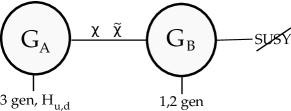
Figure 1: A diagram describing the model with $G_{A},G_{B}$ being gauge groups and $\chi,\tilde{\chi}$ being link fields.

Let us step back for a moment and consider the following representations: 

R	$SU(3)$	$SU(2)$	$U(1)$
$Q$	3	2	$1/6$
$u^{c}$	$\bar{\bf 3}$	1	$-2/3$
$d^{c}$	$\bar{\bf 3}$	1	$1/3$
$L$	1	2	$-1/2$
$e^{c}$	1	1	$1$

Without any prejudices we can now consider couples of link fields $\chi_{R},\tilde{\chi}_{R}$, in the representation $(R,\bar{R})$ and $(\bar{R},R)$ of the group $G_{A}\times G_{B}$, and we choose $G_{A},G_{B}=SU(3)\times SU(2)\times U(1)$, for simplicity. $R$ can be one of the representations given in the table above. A single couple of link fields is in general not sufficient for providing all the SSM Yukawa couplings and hence we propose the skeletal link of fig. 1 to consist of at least two couples of fields e.g. $\{\chi_{R_{1}},\chi_{R_{2}},\cdots\}$. A single couple of bifundamental link fields of $SU(5)$ corresponds in our notation to $\{\chi_{d^{c}},\chi_{L}\}$, which is the case studied in detail in [14], while [6] considered the case of $\{\chi_{Q},\chi_{L}\}$.

When a choice is made, the link fields give rise to Yukawa textures for the fermions of the SM in terms of higher dimension operators. As an example, we can have

$$\frac{\lambda^{u}_{ij}}{\Lambda^{2}}Q_{i}H_{u}u_{j}^{c}\chi_{u^{c}}\chi_{Q}\,,$$ (1)

where $i,j=1,2$ are generation indices and the labels on the $\chi$s denote the representation under which they transform. This particular example generates a Yukawa matrix

$$Y^{u}_{ij}=\lambda^{u}_{ij}\epsilon_{u}\epsilon_{Q}\,,\qquad i,j=1,2\,.$$ (2)

Here we have defined $\epsilon_{R}\equiv v_{R}/\Lambda$, where $v_{R}$ is the VEV of $\chi_{R},\tilde{\chi}_{R}$ and $\Lambda$ is the UV scale of flavor dynamics. Similar operators are needed for the complete set of three generations, as well as for the down and lepton sectors.

To break $G_{A}\times G_{B}$ to the SM group $G_{\rm SM}$ we must include link fields charged under both $SU(3)$ and $SU(2)$. Moreover, to choose the ideal representations for the link fields we need to check if they reproduce naturally the quark masses and the CKM matrix. The minimal choice required for these purposes is one of the following five possibilities: $\{\chi_{L},\chi_{u^{c}}\}$, $\{\chi_{L},\chi_{d^{c}}\}$, $\{\chi_{Q},\chi_{L}\}$, $\{\chi_{Q},\chi_{u^{c}}\}$, $\{\chi_{Q},\chi_{d^{c}}\}$. It turns out that one can easily obtain such textures with all $\lambda^{u}_{ij},\lambda^{d}_{ij}$ generically being close to one, in the cases $\{\chi_{Q},\chi_{u^{c}}\}$ and $\{\chi_{Q},\chi_{d^{c}}\}$. The case $\{\chi_{Q},\chi_{L}\}$ requires an extra hierarchy of a factor of roughly 3 between the different couplings relative to the previous ones, while the choices $\{\chi_{L},\chi_{u^{c}}\}$, $\{\chi_{L},\chi_{d^{c}}\}$ require an extra factor of 20 tuning, instead.

Interestingly, the ${\bf 10}$ of $SU(5)$ decomposes under $SU(3)\times SU(2)\times U(1)$ as $Q\oplus u^{c}\oplus e^{c}$. The texture of the quark sector is blind to the inclusion of the link $\chi_{e^{c}}$ and hence does not alter the above argument. The effect on the sleptonic sector is a possible increase in the slepton masses which can be useful for the RG evolution not to drive the stau tachyonic. In the following we will thus focus on the choice of link fields $\{\chi_{Q},\chi_{u^{c}},\chi_{e^{c}}\}$.

Since we include higher dimension operators, B or L-violating operators, such as

$$\frac{QQQL}{\Lambda}\,,\qquad\frac{u^{c}u^{c}d^{c}e^{c}}{\Lambda}\,,\qquad\frac{LH_{u}LH_{u}}{\Lambda}\,,$$ (3)

cannot be avoided by imposing R-parity. If $\Lambda$ is below the GUT scale, we are forced to impose either baryon or lepton number conservation to prevent proton decay. The last operator in eq. (3) could be envisioned to provide neutrino masses via a seesaw mechanism if $\Lambda$ is bigger than roughly $10^{13}$ GeV. In the following we will usually impose both R-parity as well as baryon and lepton number conservation.

2.1 Two nodes model with link fields $\{\chi_{Q},\chi_{u^{c}},\chi_{e^{c}}\}$

Due to the discussion above, we consider the link fields $\{\chi_{Q},\chi_{u^{c}},\chi_{e^{c}}\}$. The Yukawa textures in this case are

$$Y^{u}\sim\begin{pmatrix}\epsilon_{u}\epsilon_{Q}&\epsilon_{u}\epsilon_{Q}&\epsilon_{Q}\\ \epsilon_{u}\epsilon_{Q}&\epsilon_{u}\epsilon_{Q}&\epsilon_{Q}\\ \epsilon_{u}&\epsilon_{u}&1\end{pmatrix}\,,\qquad Y^{d}\sim\begin{pmatrix}\epsilon_{u}\epsilon_{Q}&\epsilon_{u}\epsilon_{Q}&\epsilon_{Q}\\ \epsilon_{u}\epsilon_{Q}&\epsilon_{u}\epsilon_{Q}&\epsilon_{Q}\\ \epsilon_{Q}^{2}&\epsilon_{Q}^{2}&1\end{pmatrix}\,,\qquad Y^{e}\sim\begin{pmatrix}\epsilon_{u}\epsilon_{Q}&\epsilon_{u}\epsilon_{Q}&\epsilon_{u}\epsilon_{Q}\\ \epsilon_{u}\epsilon_{Q}&\epsilon_{u}\epsilon_{Q}&\epsilon_{u}\epsilon_{Q}\\ \epsilon_{e}&\epsilon_{e}&1\end{pmatrix}\,,$$ (4)

where each element of the matrices is multiplied by the coefficient $\lambda^{u,d,e}_{ij}$, respectively. For randomly chosen order one coefficients, generically this texture predicts the following ratios

$$\frac{m_{u}}{m_{t}}\sim\frac{m_{c}}{m_{t}}\sim\frac{m_{d}}{m_{b}}\sim\frac{m_{s}}{m_{b}}\sim\frac{m_{e}}{m_{\tau}}\sim\frac{m_{\mu}}{m_{\tau}}\sim\mathcal{O}(\epsilon_{u}\epsilon_{Q})\,,\qquad\frac{m_{t}}{m_{b}}\sim\frac{m_{t}}{m_{\tau}}\sim\tan\beta\,,$$ (5)

explaining only the mass hierarchy between the second and third generations, whereas the hierarchy between the first and second generations can be reproduced by tuning the coefficients in such a way that the first two rows are nearly parallel vectors. The optimal value of the $\epsilon$s can be read off the mass ratio $m_{s}/m_{b}$ to be roughly $\epsilon_{Q}\simeq\epsilon_{u}\simeq 1/10$. With these values, the mass hierarchy in each sector – the up-type quarks, down-type quarks and leptons – is reasonable and, moreover, for a sufficiently large $\tan\beta$, the ratio between the down-type quark and lepton masses to the up-type masses is also reasonable.

Note that by not imposing lepton number conservation at the scale $\Lambda$, a neutrino mass matrix is also generated (in flavor basis):

$$m_{\nu}\sim\frac{v_{\rm ew}^{2}}{\Lambda}\begin{pmatrix}\epsilon_{u}^{2}\epsilon_{Q}^{2}&\epsilon_{u}^{2}\epsilon_{Q}^{2}&\epsilon_{u}\epsilon_{Q}\\ \epsilon_{u}^{2}\epsilon_{Q}^{2}&\epsilon_{u}^{2}\epsilon_{Q}^{2}&\epsilon_{u}\epsilon_{Q}\\ \epsilon_{u}\epsilon_{Q}&\epsilon_{u}\epsilon_{Q}&1\end{pmatrix}\,,\qquad v_{\rm ew}=174\,{\rm GeV}\,.$$ (6)

Even for $\Lambda\sim 10^{14}\,{\rm GeV}$, which potentially could produce viable neutrino masses, the matrix $m_{\nu}$ requires some tuning to reduce the big hierarchy in the masses and improve the lack of large mixing angles.

The link fields give rise to the masses of the SM fermions, via $\Lambda$-suppressed terms, but we also need to ensure that they decouple from the SM, ideally by a similar effect. To avoid Landau poles they should have masses at least of the order of their VEVs, $\langle\chi_{R}\rangle=\langle\tilde{\chi}_{R}\rangle=v_{R}$. Assuming that the superpotential for the link fields is indeed generated by physics at the UV scale $\Lambda$, it takes the form

$${\cal W}= -\mu_{Q}\,\chi^{\alpha i}_{\beta j}\tilde{\chi}^{\beta j}_{\alpha i}-\mu_{u}\,\chi^{\alpha}_{\beta}\tilde{\chi}^{\beta}_{\alpha}-\mu_{e}\,\chi\tilde{\chi}$$

$$+\frac{\chi^{\alpha i}_{\beta j}\tilde{\chi}^{\beta j}_{\gamma s}\chi^{\gamma s}_{\sigma r}\tilde{\chi}^{\sigma r}_{\alpha i}}{\Lambda}+\frac{\chi^{\alpha i}_{\beta j}\tilde{\chi}^{\beta r}_{\alpha t}\chi^{\gamma t}_{\sigma r}\tilde{\chi}^{\sigma j}_{\gamma i}}{\Lambda}+\frac{\chi^{\alpha i}_{\beta j}\tilde{\chi}^{\sigma j}_{\gamma i}\chi^{\gamma}_{\sigma}\tilde{\chi}^{\beta}_{\alpha}}{\Lambda}+\frac{\chi^{\alpha}_{\beta}\tilde{\chi}^{\beta}_{\gamma}\chi^{\gamma}_{\sigma}\tilde{\chi}^{\sigma}_{\alpha}}{\Lambda}+\frac{(\chi\tilde{\chi})^{2}}{\Lambda}\,,$$ (7)

where the field $\chi^{\alpha i}_{\beta j}$ transforms as $Q$, with $\alpha$ the $SU(3)$ index and $i$ the $SU(2)$ index under the group $G_{A}$, and as $\bar{Q}$ for $\beta,j$ under the group $G_{B}$. The field $\chi^{\alpha}_{\beta}$ transforms as $\bar{u^{c}}$ under the group $G_{A}$ and as $u^{c}$ under the group $G_{B}$. Finally, $\chi$ is a singlet with charge $-1$ under $U(1)_{A}$ and $1$ under $U(1)_{B}$. The fields with tildes transform under the conjugate representation with respect to the fields without tildes. This is not the most general superpotential, but it is sufficient to break $G_{A}\times G_{B}$ to $G_{\rm SM}$ as well as to give mass to all the link field components which are not eaten by the super-Higgs mechanism. We take the coefficients of the irrelevant terms in the above superpotential to be equal as an illustrative example. At the minimum where $G_{A}\times G_{B}\to G_{\rm SM}$, we have

$$\langle\chi^{\alpha i}_{\beta j}\rangle=v_{Q}\delta^{\alpha}_{\beta}\delta^{i}_{j}\,,\qquad\langle\chi^{\alpha}_{\beta}\rangle=v_{u}\delta^{\alpha}_{\beta}\,,\qquad\langle\chi\rangle=v_{e}\,,$$ (8)

where the VEVs $v_{R}$ are related to $\mu_{R}$ in eq. (7) via

$$\mu_{Q}=\frac{14v_{Q}^{2}+3v_{u}^{2}}{\Lambda}\,,\qquad\mu_{u}=\frac{6v_{Q}^{2}+2v_{u}^{2}}{\Lambda}\,,\qquad\mu_{e}=\frac{v_{e}^{2}}{\Lambda}\,.$$ (9)

The spectrum obtained at this minimum of the potential, for equal VEVs, is as follows. An (${\bf 8},{\bf 1}$) and a (${\bf 1},{\bf 3}$) have masses $4\epsilon v$; two (${\bf 8},{\bf 1}$)’s have masses $5\epsilon v$ and $9\epsilon v$, respectively; two (${\bf 8},{\bf 3}$)’s have masses $11\epsilon v$ and $15\epsilon v$, respectively; and, finally, four singlets have masses $\{1.3\epsilon v,4\epsilon v,4\epsilon v,30.7\epsilon v\}$. Since we take $\epsilon\simeq 1/10$, most of the matter acquires a mass of order $v$. There are still remaining an (${\bf 8},{\bf 1}$), a (${\bf 1},{\bf 3}$) and one singlet, which acquire a mass via the super-Higgs mechanism. In addition, there is a massless Goldstone boson coming from a global $U(1)$ symmetry under which $\chi$ has charge $1$ and $\tilde{\chi}$ has charge $-1$. We can get rid of this state by introducing e.g. the following term in the superpotential: $\epsilon_{\alpha_{1}\alpha_{2}\alpha_{3}}\epsilon^{\beta_{1}\beta_{2}\beta_{3}}\chi^{\alpha_{1}}_{\beta_{1}}\chi^{\alpha_{2}}_{\beta_{2}}\chi^{\alpha_{3}}_{\beta_{3}}\chi\chi/\Lambda^{2}$.

2.2 RG evolution

Let us first discuss the various scales in the problem. We found that the $\epsilon$s should be of order $1/10$, which means that $\Lambda$ is only an order of magnitude bigger than $v$. The mass-squared matrix of the gauge bosons is

$$\mathcal{M}^{2}_{V_{k}} =2v_{k}^{2}\begin{pmatrix}g_{A_{k}}^{2}&-g_{A_{k}}g_{B_{k}}\\ -g_{A_{k}}g_{B_{k}}&g_{B_{k}}^{2}\end{pmatrix}\,,$$ (10)

$$v_{1}^{2} \equiv\frac{v_{Q}^{2}}{5}+\frac{8v_{u}^{2}}{5}+\frac{6v_{e}^{2}}{5}\,,\qquad v_{2}^{2}\equiv 3v_{Q}^{2}\,,\qquad v_{3}^{2}\equiv 2v_{Q}^{2}+v_{u}^{2}\,.$$ (11)

Its zero eigenvalues amount to the SM gauge particles, while the heavy gauge bosons have masses

$$m_{v_{k}}^{2}=2\left(g_{A_{k}}^{2}+g_{B_{k}}^{2}\right)v_{k}^{2}\,,$$ (12)

where $k=1,2,3$ denotes the gauge groups $U(1)$, $SU(2)$ and $SU(3)$, respectively. A comment about the group theoretic data specifying our choice of representations of the link fields is in store, viz. it is encoded in the coefficients of the VEVs in eq. (11). At the Higgsing scale $m_{v}$, which we approximate by $3v$, the SM gauge couplings are given in terms of the gauge couplings $g_{A,B}$ by

$$\frac{1}{g_{k}^{2}}=\frac{1}{g_{A_{k}}^{2}}+\frac{1}{g_{B_{k}}^{2}}\ .$$ (13)

Assuming for simplicity that the components of the link fields all acquire a mass of order $v$, then below the scale $v$ the running of the gauge couplings $g_{k}$ is given by that of the MSSM, i.e.

$$\frac{d\alpha^{-1}_{k}}{dt}=-\frac{b_{k}}{2\pi}\,,\qquad b_{1}=\frac{33}{5}\,,\qquad b_{2}=1\,,\qquad b_{3}=-3\,.$$ (14)

Now, from the scale $v$ up to $m_{v}\sim 3v$, the $\beta$-function coefficients become

$$b_{1}=\frac{33}{5}\,,\qquad b_{2}=35\,,\qquad b_{3}=24\,,$$ (15)

where the contribution to $b_{3}$ corresponds to $9$ adjoints, whereas to $b_{2}$ it is analogous to $17$ adjoints. This change in the $\beta$-functions is rather drastic; for instance, a factor of $3$ running in energy decreases $\alpha_{2,3}^{-1}$ by $6$ and $4$, respectively.

Above the Higgsing scale, the $\beta$-function coefficients are split into two sets, corresponding to the two gauge groups depicted in fig. 1, and read

$$b_{A_{1}}=\frac{49}{5}\,,\qquad b_{A_{2}}=15\,,\qquad b_{A_{3}}=8\,,\qquad b_{B_{1}}=\frac{56}{5}\,,\qquad b_{B_{2}}=16\,,\qquad b_{B_{3}}=10\,.$$ (16)

The contribution from the link fields is $36/5$ to $b_{1}$, $18$ to $b_{2}$ and $15$ to $b_{3}$. These large values of the $\beta$-function coefficients result in the fact that the gauge couplings run into Landau poles rather quickly. Hence, the region of parameter space corresponding to weakly coupled gaugino mediation ($M\gg m_{v}$) is somewhat far fetched. Models which do not contain the link field $\chi_{Q}$ do not suffer as severely from fast running as is the case here.

As already mentioned, two other regimes are possible in our model, viz. $M\sim m_{v}$ and $M\ll m_{v}$. The case $M\sim m_{v}$, which is our main interest, provides a mild hierarchy of sparticle masses, i.e. the first two generations of squarks acquire a mass which is a factor of a few larger than that of the third generation. The other case, $M\ll m_{v}$, gives rise to a gauge mediation sparticle spectrum, which is nearly flavor blind, and hence flavor constraints are satisfied trivially. However, recent collider limits place more restrictive bounds in this case. Finally, the scale $m_{v}$ can be anywhere between about $10^{5}$ GeV and the Planck scale, but if we insist on gauge coupling unification it should be placed near the GUT scale.

2.3 Sparticle spectrum

The sfermion masses in the type of setup discussed above have been studied in detail in [29, 30, 31, 32, 33]. For simplicity, we restrict to a minimal messenger sector realized by coupling an F-term spurion $S$ to a single pair of messengers, $T,\tilde{T}$, in the ${\bf 5}$ and $\bar{\bf 5}$ of $SU(5)$, via

$$\mathcal{W}_{T}=ST\tilde{T}\,,\qquad\langle S\rangle=M+\theta^{2}F\,.$$ (17)

We introduce the variables

$$x\equiv\frac{F}{M^{2}}\ ,\qquad y_{k}\equiv\frac{m_{v_{k}}}{M}\ ,\qquad k=1,2,3\ .$$ (18)

The gaugino masses are given by those of minimal gauge mediation [34]:

$$m_{\tilde{g}_{k}}=\frac{\alpha_{k}}{4\pi}\frac{F}{M}n_{k}\,q(x)\,,\qquad q(x)=\frac{1}{x^{2}}\left[(1+x)\log(1+x)+(1-x)\log(1-x)\right]\,,$$ (19)

where $\alpha_{k}^{-1}=4\pi/g_{A_{k}}^{2}+4\pi/g_{B_{k}}^{2}$ and $n_{k}$ is the Dynkin index of the messenger field.

The sfermion masses are given in eq. (4.2) of [33],

$$m_{\tilde{f}_{l}}^{2}=2\sum_{k=1}^{3}\left(\frac{\alpha_{k}}{4\pi}\right)^{2}\left(\frac{F}{M}\right)^{2}\,C_{2k}^{\tilde{f}}\,n_{k}\mathcal{E}^{l}(x,y_{k})\ ,$$ (20)

where $C_{2k}^{\tilde{f}}$ is the quadratic Casimir of the representation under which the sfermion ${\tilde{f}}$ transforms, while the index $l$ runs over generations. The function $\mathcal{E}^{l}$ for the first and second generation is given by

$$\mathcal{E}^{1,2}(x,y,\lambda_{2}) =\frac{1}{x^{2}}\bigg{[}\alpha_{0}(x)-\left(1-\lambda_{2}^{2}\right)\alpha_{1}(x,y)-(1-\lambda_{2})^{2}y^{2}\alpha_{2}(x,y)-\frac{2(1-\lambda_{2})}{y^{2}}\beta_{-1}(x)+\beta_{0}(x)$$

$$\phantom{=\frac{1}{x^{2}}\bigg{[}\ }+\frac{2(1-\lambda_{2})}{y^{2}}\beta_{1}(x,y)+(1-\lambda_{2})^{2}\beta_{2}(x,y)\bigg{]}\,,\qquad\lambda_{2}\equiv\frac{g^{2}_{B_{k}}}{g^{2}_{k}}\,,$$ (21)

whereas for the third generation it reads

$$\mathcal{E}^{3}(x,y)=\frac{1}{x^{2}}\left[\alpha_{0}(x)-\alpha_{1}(x,y)-y^{2}\alpha_{2}(x,y)-\frac{2}{y^{2}}\beta_{-1}(x)+\beta_{0}(x)+\frac{2}{y^{2}}\beta_{1}(x,y)+\beta_{2}(x,y)\right]\,.$$ (22)

The $\alpha$s and $\beta$s are defined in Appendix A of [33]. The soft mass of the link field is also given by eq. (20), with $\mathcal{E}^{\rm link}=\mathcal{E}^{1}+\mathcal{E}^{3}$ and an appropriate quadratic Casimir (see [33] for details).

Finally, we present an example of the spectrum for low-scale as well as for high-scale mediation in table 1. Here we have assumed that the mass of all the link fields is near $v$ and we have used eq. (15) for the gauge couplings as well as two-loop corrections to the sfermion masses coming from the link field soft masses [35]. The RG evolution from the scale $v$ down to the weak scale and the determination of the pole masses were done using SOFTSUSY [36].

	$M=5\times 10^{5}$	$M=10^{15}$
$\tan\beta=20$	$F/M=1.6\times 10^{5}$	$F/M=1.6\times 10^{5}$
$(\alpha^{-1}_{B_{1}},\alpha^{-1}_{B_{2}},\alpha^{-1}_{B_{3}})$	$(30,13,5)$	$(10,10,10)$
$(y_{1},y_{2},y_{3})$	$(1.4,1.9,2.8)$	$(1.9,2.0,2.1)$
$(v_{Q},v_{u},v_{e})$	$(0.55M,0.55M,0.55M)$	$(0.55M,0.55M,0.55M)$
$m_{\tilde{g}}$	$1287$	$1218$
$m_{\tilde{\chi}_{0}}$	$(217,416,569,590)$	$(209,407,681,692)$
$m_{\tilde{\chi}_{\pm}}$	$(416,589)$	$(406,692)$
$(m_{\tilde{u}_{L}},m_{\tilde{d}_{L}},m_{\tilde{u}_{R}},m_{\tilde{d}_{R}})$	$(3241,3242,3094,3085)$	$(2279,2280,2024,1925)$
$(m_{\tilde{t}_{1}},m_{\tilde{t}_{2}},m_{\tilde{b}_{1}},m_{\tilde{b}_{2}})$	$(1114,1218,1195,1222)$	$(833,1063,1018,1051)$
$(m_{\tilde{e}_{R}},m_{\tilde{e}_{L}},m_{\tilde{\nu}_{e}})$	$(420,1005,1002)$	$(1088,1373,1370)$
$(m_{\tilde{\tau}_{1}},m_{\tilde{\tau}_{2}},m_{\tilde{\nu}_{\tau}})$	$(111,309,289)$	$(260,468,466)$
$(m_{h_{0}},m_{H_{0}},m_{A_{0}},m_{H_{\pm}})$	$(115,604,604,609)$	$(115,775,775,779)$
$\mu$	$581$	$694$

Table 1: Sparticle pole masses in units of GeV in numerical examples, for $\tan\beta=20$ and a single messenger. $\epsilon_{Q,u}$ are taken to be $0.1$.

2.4 Flavor constraints

So far, we have constructed a model which gives rise to an inverted hierarchy of squark masses and chose link fields which produce the measured quark masses and the observed CKM matrix naturally. Yet, we should check if the model satisfies the current flavor constraints. The most stringent constraints are due to CP-violating FCNCs, implying that a couple of complex phases must be rather small – at the percent level. Constraints from meson oscillations are somewhat easier to satisfy since our model has degenerate sfermion masses for the first two generations, which ameliorate the danger of unacceptable $K-\bar{K}$ and $D-\bar{D}$ mixing. Constraints due to $B_{d}-\bar{B}_{d}$ mixing turn out to be the most important in this model; less important are those due to $B_{s}-\bar{B}_{s}$ mixing. Next, we establish that in a rather large regime of parameter space, the meson mixing constraints are satisfied, as a result of the sparticle mass hierarchy as well as quark-squark alignment.

Let us first define the fermion mass matrices $m_{u}=Y^{u}v_{u}$, $m_{d}=Y^{d}v_{d}$, $m_{e}=Y^{e}v_{d}$. We can rotate to the mass eigenstate basis via

$$(U_{L}^{u})^{\dagger}m_{u}U_{R}^{u}=D^{u}\,,\qquad(U_{L}^{d})^{\dagger}m_{d}U_{R}^{d}=D^{d}\,,$$ (23)

in terms of which the CKM matrix is $V_{\rm CKM}=(U_{L}^{u})^{\dagger}U_{L}^{d}$. The most general Yukawa matrices which give correct quark masses as well as the $V_{\rm CKM}$ can be written as

$$Y^{u}v_{u}=AV_{\rm CKM}^{\dagger}D^{u}B\,,\qquad Y^{d}v_{d}=AD^{d}C\,,\qquad v_{u,d}\equiv\langle H^{0}_{u,d}\rangle\,,\qquad\tan\beta\equiv\frac{v_{u}}{v_{d}}\,,$$ (24)

with $A$, $B$ and $C$ being arbitrary $SU(3)$ matrices. Hence, it follows that by ignoring complex (CP) phases we are dealing with three 3-spheres of parameter space. We find $A,B,C$ in such a way that the coefficients $\lambda^{u,d}_{ij}$ (see eq. (2)) are all in a certain range, say $[0.11,1.1]$. There are a lot of such similar solutions, all giving rise to the measured fermion masses and CKM matrix but not necessarily to the same flavor constraints, which we shall analyze next.

Consider the sfermion mass-squared matrix

$$\mathcal{M}^{2}_{\tilde{f}}=\begin{pmatrix}(\mathcal{M}^{2}_{\tilde{f}})_{LL}&(\mathcal{M}^{2}_{\tilde{f}})_{LR}\\ (\mathcal{M}^{2}_{\tilde{f}})_{RL}&(\mathcal{M}^{2}_{\tilde{f}})_{RR}\\ \end{pmatrix}\,,\qquad\tilde{f}=\tilde{u},\tilde{d},\tilde{e}\,\ .$$ (25)

The off-diagonal blocks, corresponding to LR/RL mixing, can be neglected in our model, because the trilinear couplings ($A$-terms) are negligible. Hence, the diagonalization of $\mathcal{M}^{2}_{\tilde{f}}$ splits into the diagonalization of the two independent LL and RR $3\times 3$ blocks:

$$D_{L,\tilde{f}}^{2}=(W_{L}^{\tilde{f}})^{\dagger}(\mathcal{M}_{\tilde{f}}^{2})_{LL}W_{L}^{\tilde{f}}\,,\qquad D_{R,\tilde{f}}^{2}=(W_{R}^{\tilde{f}})^{\dagger}(\mathcal{M}_{\tilde{f}}^{2})_{RR}W_{R}^{\tilde{f}}\,,$$ (26)

in terms of which the quark-squark-gluino mixing matrices are given by

$$(Z^{f}_{L})_{ij}=-(U^{f}_{L})^{{\dagger}}_{ik}\,(W_{L}^{\tilde{f}})_{kj}\,,\qquad(Z^{f}_{R})_{ij}=(U^{f}_{R})^{{\dagger}}_{ik}\,(W_{R}^{\tilde{f}})_{kj}\,,\qquad f=u,d\,,$$ (27)

with $i,j,k=1,2,3$.

Let us now describe the calculation of the FCNC contributions to the $K-\bar{K}$ mixing in our model. The squark-gluino box contribution to the neutral kaon mixing can be parametrized by

$$\mathcal{H}=C_{1}O_{1}+\tilde{C}_{1}\tilde{O}_{1}+C_{4}O_{4}+C_{5}O_{5}\,,$$ (28)

where

$$O_{1}=\bar{d}_{L}^{\alpha}\gamma_{\mu}s_{L}^{\alpha}\bar{d}_{L}^{\beta}\gamma^{\mu}s_{L}^{\beta}\,,\qquad O_{4}=\bar{d}_{R}^{\alpha}s_{L}^{\alpha}\bar{d}_{L}^{\beta}s_{R}^{\beta}\,,\qquad O_{5}=\bar{d}_{R}^{\alpha}s_{L}^{\beta}\bar{d}_{L}^{\beta}s_{R}^{\alpha}\,.$$ (29)

$\tilde{O}_{1}$ is related to $O_{1}$ by left and right interchange. There are generically more operators (i.e. $O_{2},O_{3},\tilde{O}_{2},\tilde{O}_{3}$) which are negligible here due to the negligible $A$-terms.

The coefficients in front of the operators taken at the superpartner scale are given by [37, 38, 39]

$$C_{1} =\alpha_{s}^{2}\sum_{i,j=1}^{3}\left(\frac{11}{36}A_{ij}^{LL}+\frac{1}{9}B_{ij}^{LL}\right)(Z^{d}_{L})^{*}_{1i}(Z^{d}_{L})_{2i}(Z^{d}_{L})^{*}_{1j}(Z^{d}_{L})_{2j}\,,$$

$$\tilde{C}_{1} =\alpha_{s}^{2}\sum_{i,j=1}^{3}\left(\frac{11}{36}A_{ij}^{RR}+\frac{1}{9}B_{ij}^{RR}\right)(Z^{d}_{R})^{*}_{1i}(Z^{d}_{R})_{2i}(Z^{d}_{R})^{*}_{1j}(Z^{d}_{R})_{2j}\,,$$

$$C_{4} =\alpha_{s}^{2}\sum_{i,j=1}^{3}\left(-\frac{1}{3}A_{ij}^{LR}+\frac{7}{3}B_{ij}^{LR}\right)(Z^{d}_{L})^{*}_{1i}(Z^{d}_{L})_{2i}(Z^{d}_{R})^{*}_{1j}(Z^{d}_{R})_{2j}\,,$$

$$C_{5} =\alpha_{s}^{2}\sum_{i,j=1}^{3}\left(\frac{5}{9}A_{ij}^{LR}+\frac{1}{9}B_{ij}^{LR}\right)(Z^{d}_{L})^{*}_{1i}(Z^{d}_{L})_{2i}(Z^{d}_{R})^{*}_{1j}(Z^{d}_{R})_{2j}\,,$$ (30)

where the $3\times 3$ matrices $A^{MN},B^{MN}$, $M,N=L,R$, are given by

$$A_{ij}^{MN} =\frac{m_{\tilde{g}}^{2}}{(m_{i}^{2}-m_{\tilde{g}}^{2})(m_{j}^{2}-m_{\tilde{g}}^{2})}+\frac{m_{i}^{4}}{(m_{i}^{2}-m_{j}^{2})(m_{i}^{2}-m_{\tilde{g}}^{2})^{2}}\log\left(\frac{m_{i}^{2}}{m_{\tilde{g}}^{2}}\right)+\frac{m_{j}^{4}}{(m_{j}^{2}-m_{i}^{2})(m_{j}^{2}-m_{\tilde{g}}^{2})^{2}}\log\left(\frac{m_{j}^{2}}{m_{\tilde{g}}^{2}}\right)\,,$$

$$B_{ij}^{MN} =\frac{m_{\tilde{g}}^{2}}{(m_{i}^{2}-m_{\tilde{g}}^{2})(m_{j}^{2}-m_{\tilde{g}}^{2})}+\frac{m_{i}^{2}m_{\tilde{g}}^{2}}{(m_{i}^{2}-m_{j}^{2})(m_{i}^{2}-m_{\tilde{g}}^{2})^{2}}\log\left(\frac{m_{i}^{2}}{m_{\tilde{g}}^{2}}\right)+\frac{m_{j}^{2}m_{\tilde{g}}^{2}}{(m_{j}^{2}-m_{i}^{2})(m_{j}^{2}-m_{\tilde{g}}^{2})^{2}}\log\left(\frac{m_{j}^{2}}{m_{\tilde{g}}^{2}}\right)\,,$$

with $m_{i}\equiv\big{(}D_{M,\tilde{d}}\big{)}_{ii}$, $m_{j}\equiv\big{(}D_{N,\tilde{d}}\big{)}_{jj}$ (see eq. (26)) and $m_{\tilde{g}}$ is the gluino mass. These operators should be evolved by RG equations down to approximately the hadronic scale $\mu=2{\rm GeV}$. This can be done using the so-called magic numbers; see e.g. [40]. Finally, we can evaluate the contribution to the $K_{L}-K_{S}$ mass difference as

$$\Delta m_{K}=2\,{\rm Re}\left\langle\left.K^{0}\right|\mathcal{H}\left|\bar{K}^{0}\right.\right\rangle\,.$$ (31)

Constraints due to $B_{d}-\bar{B}_{d}$ and $B_{s}-\bar{B}_{s}$ mixing can also be evaluated using eq. (30), by substituting $(Z^{d}_{L,R})_{1i}$ and $(Z^{d}_{L,R})_{2i}$ with $(Z^{d}_{L,R})_{1i}$ and $(Z^{d}_{L,R})_{3i}$, respectively (for $B_{d}-\bar{B}_{d}$) or with $(Z^{d}_{L,R})_{2i}$ and $(Z^{d}_{L,R})_{3i}$, respectively (for $B_{s}-\bar{B}_{s}$). The constraints coming from $D-\bar{D}$ mixing are similarly evaluated using eq. (30), by changing $Z^{d}$ to $Z^{u}$. The magic numbers for $B_{q}-\bar{B}_{q}$ mixing are given in [42], while those for $D-\bar{D}$ mixing are in [41]. The experimental constraints that we have used are shown in table 2.

Constraints from $b\rightarrow s\gamma$ (due to the gluino-squark loop) have been computed using expressions in [43, 44]; these constraints are linearly enhanced by $\tan\beta$ and are in principle important especially if there is interference between the new physics and the SM contributions [45]. We found that these constraints are always satisfied in our model.

	Experimental value
$\Delta m_{K^{0}}$	$3.483\times$	$10^{-12}\,{\rm MeV}$
$\Delta m_{D^{0}}$	$1.57\times$	$10^{-11}\,{\rm MeV}$
$\Delta m_{B^{0}}$	$3.337\times$	$10^{-10}\,{\rm MeV}$
$\Delta m_{B_{s}}$	$1.163\times$	$10^{-8}\,{\rm MeV}$
$|\epsilon_{K}|$	$2.228\times$	$10^{-3}$
$|\epsilon_{K}^{\rm SM}|$	$1.8\times$	$10^{-3}$
$BR(b\rightarrow s\gamma)\phantom{{}^{\rm SM}}$	$(3.55\pm 0.24)\times$	$10^{-4}$
$BR(b\rightarrow s\gamma)^{\rm SM}$	$(3.15\pm 0.23)\times$	$10^{-4}$
$BR(\mu\rightarrow e\gamma)\phantom{{}^{\rm SM}}$	$<2.4\times$	$10^{-12}$

Table 2: Limits used in the FCNC analyses; $|\epsilon_{K}|$ is the measured value of the kaon $\epsilon$-parameter, while $|\epsilon_{K}^{\rm SM}|$ is a calculation of the Standard Model contribution [46]. The experimental value of $BR(b\rightarrow s\gamma)$ is for $E_{\gamma}>1.6\,{\rm GeV}$; the Standard Model calculation $BR(b\rightarrow s\gamma)^{\rm SM}$ is taken from [47].

We now return to inspecting the big parameter space of the model discussed above. We randomly choose the matrices $A,B,C$ of eq. (24) to find coefficients $\lambda^{u,d}_{ij}$ of order one, which produce the measured fermion masses and the CKM matrix elements. For concreteness, let the $\lambda$s be in a certain range, say $[0.11,1.1]$. We have done some statistics by finding random coefficients $\lambda^{u,d}_{ij}$ of the model such that all the neutral meson oscillation constraints are within the experimental bounds. For simplicity, we have used in the analysis the running fermion masses at the scale of the top mass (see e.g. table in 1 in [48]). By repeating this exercise 5,000 times we get within an accuracy of roughly $1.4\%$ that $41\%$ of randomly chosen coefficients give rise to specific model data passing all the above-mentioned flavor constraints in the case of the spectrum shown in the first column of table 1, i.e. in the low-scale mediation example. For the high-scale mediation example (with masses shown in the second column of table 1) we find by the same analysis that $45\%$ of the randomly chosen model points satisfy all the flavor constraints. This shows that the model has a large space of parameters which works out well in terms of the quark masses, the CKM matrix and flavor constraints.

If an order one complex phase is added to the rotation matrix of the right-handed squarks, constraints from CP violation are rather stringent. One constraint is coming from the $\epsilon_{K}$ parameter in the neutral kaon system,

$$\epsilon_{K}=\frac{1}{\sqrt{2}\Delta m_{K}}{\rm Im}\left.\left\langle K^{0}\right|\mathcal{H}\left|\bar{K}^{0}\right.\right\rangle\,.$$ (32)

There are $15$ phases that in principle can contribute to this observable ($9$ from $Y^{d}$, $3$ from $(\mathcal{M}_{\tilde{d}}^{2})_{LL}$ and $3$ from $(\mathcal{M}_{\tilde{d}}^{2})_{RR}$). If the masses of the first two generations of squarks are equal, we can use a symmetry space of dimension $13$ to set some of the phases to zero. This implies that only $2$ independent physical phases can contribute to $\epsilon_{K}$. The SM prediction [46], however, is rather firm (see table 2) and therefore we limit the contribution from new physics in our model to be within the difference $|\epsilon_{K}|-|\epsilon_{K}^{\rm SM}|$ which typically means that the two independent complex phases situated in the right-handed rotation matrix $U_{R}^{d}$ should be tuned at the percent level. This is left as a weak point of our model.

Flavor violations in the leptonic sector could be induced by the non-diagonal couplings in $Y^{e}$ (see eq. (4)). However, here the situation with $\mu\rightarrow e\gamma$ is rather robust, due to the degeneracy of the selectron and smuon masses; using eq. (20) in [38] as an estimate, a typical example with order one non-diagonal couplings, gives at worst about $1/30$ of the current experimental limits.

Above, we presented the results of the analysis done for $\tan\beta=20$. We have done the statistical analysis also in the case $\tan\beta=50$ and obtained similar results; the number of model points satisfying the flavor constraints increased slightly with respect to that of $\tan\beta=20$.

3 Higgs mass and naturalness

It is well known that there is some tension in the MSSM between the LEP bounds on the Higgs mass and naturalness. On the one hand, in gauge-mediated models, a stop with mass of about $1$ TeV or more is needed for feeding quantum corrections into the Higgs mass in order to raise it above $114$ GeV. On the other hand, the stop mass should not be much heavier than the weak scale in order to cut off the quadratic divergences of top loops. This tension is enhanced significantly if the Higgs is heavier. Recently, the ATLAS and CMS collaborations have presented evidence for a SM-like Higgs boson with a mass of about $125$ GeV [49, 50]. If a Higgs boson with such mass will be discovered, a stop of about $5$ TeV or above would be needed, leading to about $0.1\%$ fine tuning or worse.

The root of this little hierarchy problem is due to the fact that in the MSSM the tree-level mass of the Higgs is bounded by $m_{Z}$ and hence a big loop correction is needed. Interestingly, in our class of models there exists a natural mechanism for raising the tree-level Higgs mass, because the D-term of the heavy gauge bosons does not decouple completely in the presence of SUSY breaking. The usual MSSM D-terms are modified to [51]

$$V_{D}=\frac{g_{2}^{2}(1+\Delta_{2})}{8}\left|H_{u}^{\dagger}\sigma^{a}H_{u}+H_{d}^{\dagger}\sigma^{a}H_{d}\right|^{2}+\frac{3}{5}\frac{g_{1}^{2}(1+\Delta_{1})}{8}\left|H_{u}^{\dagger}H_{u}-H_{d}^{\dagger}H_{d}\right|^{2}\,,$$ (33)

where $\sigma^{a}$ are the Pauli matrices and $\Delta_{k}$ are given by

$$\Delta_{k}=\frac{\alpha^{-1}_{B_{k}}}{\alpha^{-1}_{A_{k}}}\frac{2m_{\chi_{k}}^{2}}{m_{v_{k}}^{2}+2m_{\chi_{k}}^{2}}\,,\qquad m_{\chi_{1}}^{2}=\frac{m^{2}_{\chi_{Q}}+8m^{2}_{\chi_{u}}+6m^{2}_{\chi_{e}}}{15}\,,\qquad m_{\chi_{2}}^{2}=m^{2}_{\chi_{Q}}\,,$$ (34)

where $m^{2}_{\chi_{R}}$ are the soft masses of the link fields. In the presence of $\Delta_{1,2}$, the usual bound $m_{h_{0}}<m_{Z}$ at tree level (which is saturated at large $\tan\beta$) is replaced by

$$m_{h_{0}}^{2}<\frac{\frac{3}{5}g_{1}^{2}(1+\Delta_{1})+g_{2}^{2}(1+\Delta_{2})}{2}\,v_{\rm ew}^{2}\,,\qquad v_{\rm ew}=174\,{\rm GeV}\,.$$ (35)

If $\Delta_{1,2}$ are of order one, this contribution is quite useful for ameliorating the little hierarchy problem. This puts an upper bound on $m_{v_{k}}$, of the order of the link-field soft masses (which are at most about $10$ TeV). A second requirement is that $\alpha^{-1}_{B_{k}}$ is not too small compared to $\alpha^{-1}_{A_{k}}$. When the link fields $\chi,\tilde{\chi}$ are bifundamentals of $SU(5)$, this mechanism can raise the Higgs mass rather effectively. For instance, remaining in the perturbative regime, for $g_{A_{k}}\approx g_{B_{k}}$ it provides a $140$ GeV Higgs with the stop mass near the TeV [24].

The main obstacle in realizing this mechanism in a model with $\chi_{Q}$ link fields is that we generically need $m_{v_{k}}\approx M$ to be far away from Landau poles, and $M$ should be at least a few $100$’s of TeV to give the right sparticle masses. Nevertheless, if we stretch the scales of the problem to the limit, this is marginally possible in the low-mediation regime; if the irrelevant operators of the superpotential (7) have large enough coefficients (of order of a few), and all the link-field matter has mass of order $m_{v}\approx 10$ TeV, a Landau pole is reached near $20m_{v}$, which is just enough to accommodate for the messengers. This corner of parameter space is in a regime where we can only marginally trust perturbative calculations. Yet, this regime is also motivated for the following reason. The condensed values of the various scales in this case, provide a possible solution to the $\mu$ problem: following the strategy of [14], we can prohibit a direct $\mu H_{u}H_{d}$ term by some symmetry, and then obtain the $\mu$-term from the operator $\chi\tilde{\chi}H_{u}H_{d}/\Lambda$; it gives the correct order of magnitude if this irrelevant operator has an order one coefficient.

Figure 2: A diagram describing a modification of the model in order to give an extra tree-level contribution to the Higgs mass, ameliorating the little hierarchy problem.

A possible alternative is shown in figure 2. We add an extra gauge group $G_{\sigma}$, taken to be $SU(2)$, and an extra set of link fields $\sigma,\tilde{\sigma}$ in the bifundamental of $SU(2)_{\sigma}\times SU(2)_{A}$. Suppose now that $\sigma,\tilde{\sigma}$ get a VEV $v_{\sigma}\approx 10^{4}$ GeV, e.g. using irrelevant operators as in the case of $\chi,\tilde{\chi}$. Assuming that $v_{\chi}\gg v_{\sigma}$ and coupling $G_{\sigma}$ to the SUSY-breaking messenger, then the link field $\sigma$ gets a gauge-mediated soft mass $m_{\sigma}$ providing the Higgs potential with a contribution as in eq. (33), with

$$\Delta_{1}=0\,,\qquad\Delta_{2}=\frac{\alpha^{-1}_{\sigma}}{\alpha^{-1}_{A_{2}}}\frac{2m_{\sigma}^{2}}{m_{v_{\sigma}}^{2}+2m_{\sigma}^{2}}\,,\qquad m_{v_{\sigma}}^{2}=2(g^{2}_{\sigma}+g_{2}^{2})v_{\sigma}^{2}\,.$$ (36)

Following [51], it might even be possible to obtain unification as well as having a heavy Higgs, by taking the VEV of $\chi$ to be near the GUT scale. Only the running of the $SU(2)$ gauge coupling is potentially affected, but the two new contributions, i.e. from the extra gauge bosons as well as from the link fields $\sigma$, cancel out. Several alternatives, generically not consistent with unification, could be considered. For instance, we could take $G_{\sigma}=U(1)$ or $SU(2)\times U(1)$, as well as various representations for $\sigma$. Other ways of achieving unification might also be a possibility here; see e.g. [52, 53].

One should note that in parameter space, the LHC Higgs production cross section could deviate from that of the Standard Model. For a recent study of this issue in the MSSM, both with and without extra D-terms, see [54]. Constraints from $b\rightarrow s\gamma$ (due to charged Higgs-top and chargino-stop loops) can be important and depend on the details of the spectrum in the Higgs sector.

Another way to achieve a heavier Higgs boson is to couple the Higgs sector to the SUSY-breaking one, in order to generate a large trilinear $A_{t}$-term at the messenger scale. For instance, this is possible if the Higgses mix with doublet messengers [55].

4 Three nodes model

To generate a hierarchy also between the first and second generations of SM fermion masses without tuning any coefficients, we consider the three-nodes extension shown in fig. 3. In this example, both the link fields $\chi,\eta$ are taken in the representations $\{\chi_{Q},\chi_{u^{c}},\chi_{e^{c}}\}$, $\{\eta_{Q},\eta_{u^{c}},\eta_{e^{c}}\}$.

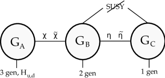
Figure 3: A diagram describing the model with $G_{A},G_{B},G_{C}$ being gauge groups and $\chi,\tilde{\chi},\eta,\tilde{\eta}$ being link fields.

Introducing higher dimension operators, as before, this model gives rise to Yukawa matrices of the form

$$Y_{u} =\begin{pmatrix}\epsilon_{u}\epsilon_{Q}\delta_{Q}\delta_{u}&\epsilon_{u}\epsilon_{Q}\delta_{Q}&\epsilon_{Q}\delta_{Q}\\ \epsilon_{u}\epsilon_{Q}\delta_{u}&\epsilon_{u}\epsilon_{Q}&\epsilon_{Q}\\ \epsilon_{u}\delta_{u}&\epsilon_{u}&1\end{pmatrix}\,,\qquad Y_{d}=\begin{pmatrix}\epsilon_{u}\epsilon_{Q}\delta_{Q}\delta_{u}&\epsilon_{u}\epsilon_{Q}\delta_{Q}&\epsilon_{Q}\delta_{Q}\\ \epsilon_{u}\epsilon_{Q}\delta_{Q}^{2}&\epsilon_{u}\epsilon_{Q}&\epsilon_{Q}\\ \epsilon_{Q}^{2}\delta_{Q}^{2}&\epsilon_{Q}^{2}&1\end{pmatrix}\,,$$ (37)

$$Y_{e} =\begin{pmatrix}\epsilon_{u}\epsilon_{Q}\delta_{Q}\delta_{u}&\epsilon_{u}\epsilon_{Q}\delta_{Q}\delta_{u}&\epsilon_{u}\epsilon_{Q}\delta_{Q}\delta_{u}\\ \epsilon_{u}\epsilon_{Q}\delta_{e}&\epsilon_{u}\epsilon_{Q}&\epsilon_{u}\epsilon_{Q}\\ \epsilon_{e}\delta_{e}&\epsilon_{e}&1\\ \end{pmatrix}\,,$$

where $\epsilon_{R}=\langle\chi_{R}\rangle/\Lambda$ and $\delta_{R}=\langle\eta_{R}\rangle/\Lambda$. The texture of $Y^{u}$ is again identical to the one realized in single-sector SUSY breaking [16, 19]; $Y^{d}$ instead is slightly different in the lower triangular part. For generic order one coefficients, $\lambda_{ij}^{u,d,e}$, these textures predict

$$\frac{m_{c}}{m_{t}}\sim\frac{m_{s}}{m_{b}}\sim\frac{m_{\mu}}{m_{\tau}}\sim\mathcal{O}(\epsilon_{u}\epsilon_{Q})\,,\qquad\frac{m_{u}}{m_{c}}\sim\frac{m_{d}}{m_{s}}\sim\frac{m_{e}}{m_{\mu}}\sim\mathcal{O}(\delta_{u}\delta_{Q})\,,\qquad\frac{m_{t}}{m_{b}}\sim\frac{m_{t}}{m_{\tau}}\sim\tan\beta\,.$$ (38)

The MSSM gauge couplings $g_{k}$ are given in terms of the gauge couplings of the unbroken theory by

$$\frac{1}{g_{k}^{2}}=\frac{1}{g_{A_{k}}^{2}}+\frac{1}{g_{B_{k}}^{2}}+\frac{1}{g_{C_{k}}^{2}}\,,$$ (39)

where $k=1,2,3$ correspond to the $U(1)$, $SU(2)$ and $SU(3)$ gauge groups, respectively. Above the Higgsing scale the gauge $\beta$-function coefficients read

$$b_{A_{1}}=\frac{49}{5},\,\,\,b_{A_{2}}=15,\,\,\,b_{A_{3}}=8,\,\,\,b_{B_{1}}=\frac{82}{5},\,\,\,b_{B_{2}}=32,\,\,\,b_{B_{3}}=23,\,\,\,b_{C_{1}}=\frac{46}{5},\,\,\,b_{C_{2}}=14,\,\,\,b_{C_{3}}=8\,.$$ (40)

Running by a factor of ten in energy decreases $\alpha_{B_{2}}^{-1}$ by an amount of about $12$, and $\alpha_{B_{3}}^{-1}$ by $10$, $\alpha_{A_{2}}^{-1},\alpha_{C_{2}}^{-1}$ by $5$ and $\alpha_{A_{3}}^{-1},\alpha_{C_{3}}^{-1}$ by $3$. Hence, the running of the gauge couplings is even faster than in the two-nodes model. The gauge couplings are running into Landau poles in about a factor of ten in energy above the Higgsing scale, and thus the regime $M\gg m_{v}$ is unattainable.

The main experimental challenge for this model is due to the constraints from $K-\bar{K}$ and $D-\bar{D}$ oscillations, which allow just for tiny differences between the first and the second generations of squark masses. For this purpose, we introduce an approximate $\mathbb{Z}_{2}$ symmetry, forcing the gauge couplings of $G_{B}$ and $G_{C}$ to be the same and also the messengers coupled to the gauge groups have the same mass and are coupled in the same way to a common SUSY-breaking spurion. In order not to break this approximate symmetry by the different running of the couplings $g_{B,C}$, one may consider adding extra matter to $G_{C}$ such that the running becomes approximately equal.

4.1 Sparticle spectrum

Let us define the quantities $v_{\epsilon k},v_{\delta k}$ in analogy with the two-nodes case in eq. (11). The mass-squared matrix of the gauge bosons is given by

$$\mathcal{M}_{V_{k}}^{2}=2\begin{pmatrix}g_{A_{k}}^{2}v_{\epsilon k}^{2}&-g_{A_{k}}g_{B_{k}}v_{\epsilon k}^{2}&0\\ -g_{A_{k}}g_{B_{k}}v_{\epsilon k}^{2}&g_{B_{k}}^{2}\left(v_{\epsilon k}^{2}+v_{\delta k}^{2}\right)&-g_{B_{k}}g_{C_{k}}v_{\delta k}^{2}\\ 0&-g_{B_{k}}g_{C_{k}}v_{\delta k}^{2}&g_{C_{k}}^{2}v_{\delta k}^{2}\end{pmatrix}\ .$$ (41)

Hence, the masses of the heavy gauge bosons are

$$(m_{v_{k}}^{\mp})^{2}=a_{k}+b_{k}\mp\sqrt{(a_{k}+b_{k})^{2}-4(g_{A_{k}}^{2}g_{B_{k}}^{2}+g_{B_{k}}^{2}g_{C_{k}}^{2}+g_{A_{k}}^{2}g_{C_{k}}^{2})v_{\epsilon k}^{2}v_{\delta k}^{2}}\,,$$ (42)

where $a_{k}\equiv(g_{A_{k}}^{2}+g_{B_{k}}^{2})v_{\epsilon k}^{2}$ and $b_{k}\equiv(g_{B_{k}}^{2}+g_{C_{k}}^{2})v_{\delta k}^{2}$.

We can again apply the results of [33]. Defining the variables

$$x=\frac{F}{M^{2}}\,,\qquad y_{k}^{-}=\frac{m_{v_{k}}^{-}}{M}\,,\qquad y_{k}^{+}=\frac{m_{v_{k}}^{+}}{M}\,,$$ (43)

the soft masses of the sfermions are given by eq. (20), where $\mathcal{E}^{l}$ is different for each generation $l=1,2,3$:

$$\mathcal{E}^{1} =n_{C_{k}}\mathcal{K}\left(x,y_{k}^{-},y_{k}^{+},2\frac{g_{B_{k}}^{2}g_{C_{k}}^{2}v_{\delta k}^{2}+g_{C_{k}}^{2}(g_{A_{k}}^{2}+g_{B_{k}}^{2})v_{\epsilon k}^{2}}{M^{2}g_{k}^{2}},\frac{g_{C_{k}}^{2}}{g_{k}^{2}}\right)+n_{B_{k}}\mathcal{K}\left(x,y_{k}^{-},y_{k}^{+},2\frac{g_{B_{k}}^{2}g_{C_{k}}^{2}v_{\delta k}^{2}}{M^{2}g_{k}^{2}},0\right)\,,$$

$$\mathcal{E}^{2} =n_{C_{k}}\mathcal{K}\left(x,y_{k}^{-},y_{k}^{+},2\frac{g_{B_{k}}^{2}g_{C_{k}}^{2}v_{\delta k}^{2}}{M^{2}g_{k}^{2}},0\right)+n_{k_{B}}\mathcal{K}\left(x,y_{k}^{-},y_{k}^{+},2\frac{g_{A_{k}}^{2}g_{B_{k}}^{2}v_{\epsilon k}^{2}+g_{B_{k}}^{2}g_{C_{k}}^{2}v_{\delta k}^{2}}{M^{2}g_{k}^{2}},\frac{g_{B_{k}}^{2}}{g_{k}^{2}}\right)\,,$$ (44)

$$\mathcal{E}^{3} =n_{C_{k}}\mathcal{K}\left(x,y_{k}^{-},y_{k}^{+},0,0\right)+n_{B_{k}}\mathcal{K}\left(x,y_{k}^{-},y_{k}^{+},2\frac{g_{A_{k}}^{2}g_{B_{k}}^{2}v_{\epsilon k}^{2}}{M^{2}g_{k}^{2}},0\right)\,,$$

where the function $\mathcal{K}$ is defined in eq. (4.14) of [33], and $n_{B_{k}}$, $n_{C_{k}}$ are Dynkin indices of the messengers coupled to $G_{B}$ and $G_{C}$, respectively. The soft masses of the gauginos are given by eq. (19), with $n_{k}=n_{B_{k}}+n_{C_{k}}$. The RG evolution down to the weak scale is done in a similar way to that of the two-nodes case.

	$M=8\times 10^{5}$	$M=10^{15}$
$\tan\beta=20$	$F/M=10^{5}$	$F/M=0.8\times 10^{5}$
$(\alpha^{-1}_{B_{1},C_{1}},\alpha^{-1}_{B_{2},C_{2}},\alpha^{-1}_{B_{3},C_{3}})$	$(15,6.5,2.5)$	$(5,5,5)$
$(v_{\epsilon Q},v_{\epsilon u},v_{\epsilon e})$	$(M/3,M/3,M)$	$(M/3,M/3,M/3)$
$(v_{\delta Q},v_{\delta u},v_{\delta e})$	$(M,M,M)$	$(M,M,M)$
$(y_{1}^{-},y_{2}^{-},y_{3}^{-})$	$(1.9,1.2,1.9)$	$(1.1,1.4,1.4)$
$(y_{1}^{+},y_{2}^{+},y_{3}^{+})$	$(3.0,4.9,7.9)$	$(5.6,5.6,5.6)$
$m_{\tilde{g}}$	$1556$	$1225$
$m_{\tilde{\chi}_{0}}$	$(264,502,615,645)$	$(203,402,645,658)$
$m_{\tilde{\chi}_{\pm}}$	$(503,644)$	$(402,658)$
$(m_{\tilde{u}_{L}},m_{\tilde{d}_{L}},m_{\tilde{u}_{R}},m_{\tilde{d}_{R}})$	$(3592,3593,3434,3428)$	$(2056,2057,1839,1754)$
$(m_{\tilde{c}_{L}},m_{\tilde{s}_{L}},m_{\tilde{c}_{R}},m_{\tilde{s}_{R}})$	$(3489,3490,3335,3329)$	$(2009,2011,1799,1718)$
$(m_{\tilde{t}_{1}},m_{\tilde{t}_{2}},m_{\tilde{b}_{1}},m_{\tilde{b}_{2}})$	$(1164,1262,1237,1278)$	$(811,1016,969,1007)$
$(m_{\tilde{e}_{R}},m_{\tilde{e}_{L}},m_{\tilde{\nu}_{e}})$	$(355,1078,1074)$	$(958,1209,1207)$
$(m_{\tilde{\mu}_{R}},m_{\tilde{\mu}_{L}},m_{\tilde{\nu}_{\mu}})$	$(337,1047,1044)$	$(928,1176,1172)$
$(m_{\tilde{\tau}_{1}},m_{\tilde{\tau}_{2}},m_{\tilde{\nu}_{\tau}})$	$(114,258,221)$	$(172,383,368)$
$(m_{h_{0}},m_{H_{0}},m_{A_{0}},m_{H_{\pm}})$	$(116,619,619,624)$	$(116,699,699,704)$
$\mu$	$627$	$658$

Table 3: Sparticle masses in units of GeV in some numerical examples (with $n_{B}=n_{C}=1$), for three nodes, $\tan\beta=20$, and $\delta_{q,u,e}=0.24$, $\epsilon_{q,u}=0.08$. In the first column, $\epsilon_{e}=3\epsilon_{q,u}$ is chosen to avoid a tachyonic stau, while in the second column $\epsilon_{e}=\epsilon_{q,u}$.

In general, even for equal gauge couplings and equal messenger sectors for $G_{B,C}$, there is a splitting between the first and second generation sfermion masses, which depends parametrically on all the gauge couplings as well as the precise values of $\epsilon_{R}$ and $\delta_{R}$. To minimize this splitting, we have chosen $\delta$ slightly larger than $\epsilon$ by a factor of $\sim 3$ (see example spectra in table 3). In several examples we have observed a tendency of a very light (or even tachyonic) stau. This problem can be ameliorated by increasing slightly the VEV of $\chi_{e^{c}}$.

4.2 Flavor Constraints

As already mentioned in the previous subsection, the main problem in this three-nodes version of our model lies in satisfying the $K-\bar{K}$ and $D-\bar{D}$ mixing constraints. It turns out that the $B_{q}-\bar{B}_{q}$ mixing constraints are nearly automatically satisfied. This is due to the improved pattern giving rise to an extra hierarchy between the first two generations. $K-\bar{K}$ and $D-\bar{D}$ mixing constraints, on the other hand, pose a bigger challenge with respect to the two-nodes model, as the first two generations of squark masses are not degenerate. To quantify how well the model works, we did the same type of statistical analysis as in the two-nodes case, viz. we calculated 5,000 model points of order one coefficients $\lambda^{Q,u,e}$ in the range $[0.11,1.2]$, and we found that $63\%$ of the points satisfy all the flavor constraints simultaneously in the case of the low-scale mediation spectrum shown in the first column of table 3. In the case of the high-scale mediation spectrum, shown in the second column of table 3, we found that $33\%$ of the model points satisfy all the flavor constraints. Hence, we conclude that even though the model potentially has problems with $K-\bar{K}$ and $D-\bar{D}$ mixing, a large part of parameter space satisfies the constraints.

Finally, as in the two nodes model, we have also redone the analysis with $\tan\beta=50$, and we found the same conclusion, i.e. the number of model points satisfying the flavor constraints increased slightly with respect to that of $\tan\beta=20$.

5 Discussion

In this work, we investigated the possibility that flavor hierarchies are explained by the pattern of allowed gauge-invariant operators which follow from a quiver-like, UV completed model. We found that, both in the two and three-nodes examples, the quark as well as the lepton masses, and the CKM matrix, are naturally derived and, moreover, this is consistent with meson mixing constraints in a considerable part of the parameter space.

Constraints from CP violation are more stringent; for the model to be consistent with the bounds on the $\epsilon_{K}$ parameter, we need to tune a couple of the complex phases at the percent level. It would be interesting to find a mechanism protecting the model, e.g. by increasing the mass of the right-handed sbottom [7].

The texture of the quarks and SM lepton sectors in our model is rather good. On the other hand, relative neutrino masses and their mixing do not come out at the correct order of magnitude; it would thus be interesting to extend the model in this direction as well. It would also be interesting to explore in detail extensions of the model which can provide extra contributions to the Higgs mass, as briefly discussed in section 3.

Finally, our observation that the $\chi_{Q}$ link field gives rise to natural textures has a simple reasoning. Clearly, we need either a $\chi_{Q}$ or a $\chi_{L}$ to provide an $SU(2)$-charged link. Now, it turns out that choosing a $\chi_{L}$ link field, the $i,j=1,2$ components of the Yukawa matrices (in the two-nodes case) are given by a single $\epsilon_{L}$, to leading order. Thus, to accommodate for the observed mass hierarchy, we need to take $\epsilon_{L}\sim 1/100$. This suppresses the quark mixings. Another effect is that coupling a $\chi_{L}$ alone to the MSSM matter and Higgs cannot generate e.g. the $3i$ elements of the Yukawa matrices, and hence suppresses the quark mixing even further. Choosing instead the $\chi_{Q}$ link field, we need at least a product of two link fields to generate a gauge-invariant coupling of the $i,j=1,2$ MSSM fields with the Higgs (see eq. (1)). On the other hand, to couple the third generation to the light ones, requires a single $\chi_{Q}$ to provide a gauge-invariant operator. Consequently, $\epsilon_{Q}$ needs to be around $1/10$ to reproduce the mass hierarchy and, moreover, the mixing is automatically sufficiently large, leading naturally to the measured CKM values.

Acknowledgments

We thank Andrey Katz and Zohar Komargodski for discussions. This work was supported in part by the BSF – American-Israel Bi-National Science Foundation, and by a center of excellence supported by the Israel Science Foundation (grant number 1665/10). SBG is supported by the Golda Meir Foundation Fund.

References

• [1] Y. Kats, P. Meade, M. Reece and D. Shih, arXiv:1110.6444 [hep-ph].
• [2] S. Dimopoulos and G. F. Giudice, Phys. Lett. B 357 (1995) 573 [hep-ph/9507282].
• [3] A. G. Cohen, D. B. Kaplan and A. E. Nelson, Phys. Lett. B 388 (1996) 588 [hep-ph/9607394].
• [4] R. Barbieri, E. Bertuzzo, M. Farina, P. Lodone and D. Pappadopulo, JHEP 1008 (2010) 024 [arXiv:1004.2256 [hep-ph]].
• [5] R. Barbieri, E. Bertuzzo, M. Farina, P. Lodone and D. Zhuridov, JHEP 1012 (2010) 070 [Erratum-ibid.  1102 (2011) 044] [arXiv:1011.0730 [hep-ph]].
• [6] R. Barbieri, G. Isidori, J. Jones-Perez, P. Lodone and D. M. Straub, Eur. Phys. J. C 71 (2011) 1725 [arXiv:1105.2296 [hep-ph]].
• [7] C. Brust, A. Katz, S. Lawrence and R. Sundrum, arXiv:1110.6670 [hep-ph].
• [8] M. Papucci, J. T. Ruderman and A. Weiler, arXiv:1110.6926 [hep-ph].
• [9] A. Delgado and M. Quiros, Phys. Rev. D 85, 015001 (2012) [arXiv:1111.0528 [hep-ph]].
• [10] C. D. Froggatt and H. B. Nielsen, Nucl. Phys. B 147 (1979) 277.
• [11] A. E. Nelson and M. J. Strassler, JHEP 0009 (2000) 030 [hep-ph/0006251].
• [12] A. E. Nelson and M. J. Strassler, JHEP 0207 (2002) 021 [hep-ph/0104051].
• [13] O. Aharony, L. Berdichevsky, M. Berkooz, Y. Hochberg and D. Robles-Llana, Phys. Rev. D 81 (2010) 085006 [arXiv:1001.0637 [hep-ph]].
• [14] N. Craig, D. Green and A. Katz, JHEP 1107 (2011) 045 [arXiv:1103.3708 [hep-ph]].
• [15] N. Arkani-Hamed, M. A. Luty and J. Terning, Phys. Rev. D 58 (1998) 015004 [hep-ph/9712389].
• [16] M. A. Luty and J. Terning, Phys. Rev. D 62 (2000) 075006 [hep-ph/9812290].
• [17] M. Gabella, T. Gherghetta and J. Giedt, Phys. Rev. D 76 (2007) 055001 [arXiv:0704.3571 [hep-ph]].
• [18] S. Franco and S. Kachru, Phys. Rev. D 81 (2010) 095020 [arXiv:0907.2689 [hep-th]].
• [19] N. Craig, R. Essig, S. Franco, S. Kachru and G. Torroba, Phys. Rev. D 81 (2010) 075015 [arXiv:0911.2467 [hep-ph]].
• [20] P. Meade, N. Seiberg and D. Shih, Prog. Theor. Phys. Suppl.  177 (2009) 143 [arXiv:0801.3278 [hep-ph]].
• [21] D. Marques, JHEP 0903 (2009) 038 [arXiv:0901.1326 [hep-ph]].
• [22] T. T. Dumitrescu, Z. Komargodski, N. Seiberg and D. Shih, JHEP 1005 (2010) 096 [arXiv:1003.2661 [hep-ph]].
• [23] D. Green, A. Katz and Z. Komargodski, Phys. Rev. Lett.  106 (2011) 061801 [arXiv:1008.2215 [hep-th]].
• [24] R. Auzzi, A. Giveon, S. B. Gudnason and T. Shacham, JHEP 1109 (2011) 108 [arXiv:1107.1414 [hep-ph]].
• [25] D. E. Kaplan, G. D. Kribs and M. Schmaltz, Phys. Rev. D 62 (2000) 035010 [hep-ph/9911293].
• [26] Z. Chacko, M. A. Luty, A. E. Nelson and E. Ponton, JHEP 0001 (2000) 003 [hep-ph/9911323].
• [27] C. Csaki, J. Erlich, C. Grojean and G. D. Kribs, Phys. Rev. D 65 (2002) 015003 [hep-ph/0106044].
• [28] H. C. Cheng, D. E. Kaplan, M. Schmaltz and W. Skiba, Phys. Lett. B 515 (2001) 395 [hep-ph/0106098].
• [29] M. McGarrie, JHEP 1011 (2010) 152 [arXiv:1009.0012 [hep-ph]].
• [30] R. Auzzi and A. Giveon, JHEP 1010 (2010) 088 [arXiv:1009.1714 [hep-ph]]; JHEP 1101 (2011) 003 [arXiv:1011.1664 [hep-ph]].
• [31] M. Sudano, arXiv:1009.2086 [hep-ph].
• [32] M. McGarrie, JHEP 1109 (2011) 138 [arXiv:1101.5158 [hep-ph]].
• [33] R. Auzzi, A. Giveon and S. B. Gudnason, JHEP 1112, 016 (2011) [arXiv:1110.1453 [hep-ph]].
• [34] S. P. Martin, Phys. Rev. D 55 (1997) 3177 [hep-ph/9608224].
• [35] S. P. Martin and M. T. Vaughn, Phys. Rev. D 50 (1994) 2282 [Erratum-ibid. D 78 (2008) 039903] [hep-ph/9311340].
• [36] B. C. Allanach, Comput. Phys. Commun.  143 (2002) 305 [hep-ph/0104145].
• [37] J. S. Hagelin, S. Kelley and T. Tanaka, Nucl. Phys.  B 415 (1994) 293.
• [38] F. Gabbiani, E. Gabrielli, A. Masiero and L. Silvestrini, Nucl. Phys.  B 477 (1996) 321 [arXiv:hep-ph/9604387].
• [39] A. E. Nelson and D. Wright, Phys. Rev.  D 56 (1997) 1598 [arXiv:hep-ph/9702359].
• [40] M. Ciuchini, V. Lubicz, L. Conti, A. Vladikas, A. Donini, E. Franco, G. Martinelli and I. Scimemi et al., JHEP 9810 (1998) 008 [hep-ph/9808328].
• [41] M. Bona et al. [UTfit Collaboration], JHEP 0803 (2008) 049 [arXiv:0707.0636 [hep-ph]].
• [42] D. Becirevic, M. Ciuchini, E. Franco, V. Gimenez, G. Martinelli, A. Masiero, M. Papinutto and J. Reyes et al., Nucl. Phys. B 634 (2002) 105 [hep-ph/0112303].
• [43] L. L. Everett, G. L. Kane, S. Rigolin, L. -T. Wang and T. T. Wang, JHEP 0201 (2002) 022 [hep-ph/0112126].
• [44] E. Lunghi and J. Matias, JHEP 0704 (2007) 058 [hep-ph/0612166].
• [45] G. F. Giudice, M. Nardecchia and A. Romanino, Nucl. Phys. B 813 (2009) 156 [arXiv:0812.3610 [hep-ph]].
• [46] A. J. Buras and D. Guadagnoli, Phys. Rev. D 78 (2008) 033005 [arXiv:0805.3887 [hep-ph]].
• [47] M. Misiak, H. M. Asatrian, K. Bieri, M. Czakon, A. Czarnecki, T. Ewerth, A. Ferroglia and P. Gambino et al., Phys. Rev. Lett.  98 (2007) 022002 [hep-ph/0609232].
• [48] K. S. Babu, arXiv:0910.2948 [hep-ph].
• [49] ATLAS Collaboration, ATLAS-CONF-2011-163
• [50] CMS Collaboration, CMS PAS HIG-11-032
• [51] P. Batra, A. Delgado, D. E. Kaplan and T. M. P. Tait, JHEP 0402 (2004) 043 [arXiv:hep-ph/0309149 [hep-ph]].
• [52] N. Arkani-Hamed, A. G. Cohen and H. Georgi, hep-th/0108089.
• [53] A. Maloney, A. Pierce and J. G. Wacker, JHEP 0606 (2006) 034 [hep-ph/0409127].
• [54] A. Arvanitaki and G. Villadoro, arXiv:1112.4835 [hep-ph].
• [55] J. L. Evans, M. Ibe and T. T. Yanagida, Phys. Lett. B 705 (2011) 342 [arXiv:1107.3006 [hep-ph]].