Scheduling Light-trails on WDM Rings

Abstract

We consider the problem of scheduling communication on optical WDM (wavelength division multiplexing) networks using the light-trails technology. We seek to design scheduling algorithms such that the given transmission requests can be scheduled using minimum number of wavelengths (optical channels). We provide algorithms and close lower bounds for two versions of the problem on an $n$ processor linear array/ring network. In the stationary version, the pattern of transmissions (given) is assumed to not change over time. For this, a simple lower bound is $c$, the congestion or the maximum total traffic required to pass through any link. We give an algorithm that schedules the transmissions using $O(c+\log{n})$ wavelengths. We also show a pattern for which $\Omega(c+\log{n}/\log\log{n})$ wavelengths are needed. In the on-line version, the transmissions arrive and depart dynamically, and must be scheduled without upsetting the previously scheduled transmissions. For this case we give an on-line algorithm which has competitive ratio $\Theta(\log{n})$. We show that this is optimal in the sense that every on-line algorithm must have competitive ratio $\Omega(\log{n})$. We also give an algorithm that appears to do well in simulation (for the classes of traffic we consider), but which has competitive ratio between $\Omega(\log^{2}n/\log\log{n})$ and $O(\log^{2}n)$. We present detailed simulations of both our algorithms.

1 Introduction

Light-trails [1] are considered to be an attractive solution to the problem of bandwidth provisioning in optical networks. One key idea in this is the use of optical shutters which are inserted into the optical fiber, and which can be configured to either let the optical signal from one segment of the fiber pass through or block it from being transmitted into the next segment. By configuring some shutters ON (signal let through) and some OFF (signal blocked), the network can be partitioned into subnetworks in which multiple communications can happen in parallel on the same light wavelength. In order to use the network efficiently, it is important to have algorithms for controlling the shutters. Notice that in the ON mode, light goes through a shutter without being first converted to an electrical signal – this is one of the major advantages of the light-trail technology.

In this paper we consider the simplest scenario: two fiber optic rings, one clockwise and one anticlockwise, passing through a set of some $n$ nodes, where typically $n<20$ because of technological considerations. At each node of a ring there are optical shutters that can either be used to block or forward the signal on each possible wavelength. The optical shutters are controlled by an auxiliary network (“out-of-band channel”). It is to be noted that this auxiliary network is typically electronic, and the shutter switching time is of the order of milliseconds as opposed to optical signals which have frequencies of Gigahertz.

For this setting we give three algorithms for controlling the shutters, or bandwidth provisioning. Our first algorithm is for stationary traffic, i.e., the communication demands between processors are known at the beginning and do not change over time. Our second and third algorithm are for dynamic traffic, i.e., transmission requests arrive and depart in an on-line manner, and a new request must be assigned light-trails without requiring modifications (or with only minimal modification) to light-trails created for currently active transmissions. For both problems, our objective is to minimize the number of wavelengths needed to accommodate the given traffic. Our results are applicable to the setting in which a fixed number of wavelengths is available as follows. If our analysis indicates that some $\lambda$ wavelengths are needed while only $\lambda_{0}$ are available, then effectively the system will have to be slowed down by a factor $\lambda/\lambda_{0}$. This is of course only one formulation; there could be other formulations which allow requests to be dropped and analyze what fraction of requests are served.

The input to the stationary problem is a matrix $B$, in which $B(i,j)$ gives the bandwidth demanded between nodes $i$ and $j$, expressed as a fraction of the bandwidth supported by a single wavelength. We give an algorithm which schedules this traffic using $O(c+\log n)$ wavelengths, where $c=\max_{k}\sum_{i,j|i\leq k<j}B(i,j)$ is the maximum total bandwidth demand, or the congestion at any link. The congestion as defined above is a lower bound, and so our algorithm can be seen to use a number of wavelengths close to the optimal. The reader may wonder why the additive $\log{n}$ term arises in the result. We show that there are communication matrices $B$ for which the congestion $c$ is small, but which yet require $\Omega(c+\log{n}/\log\log{n})$ wavelengths. In some sense, this justifies the form of our result.

For the on-line problem, we use the notion of competitive analysis [2, 3, 4]. In this, an on-line algorithm which must respond without the knowledge of the future is evaluated by comparing its performance to that of an off-line adversary, an algorithm which is given all the transmission requests at the beginning. Clearly, the off-line adversary must perform at least as well as the best on-line algorithm. We establish that our first algorithm is $\Theta(\log{n})$-competitive, i.e., it requires $\Theta(\log{n})$ times as many wavelengths as needed by the off-line adversary. We also prove that no on-line algorithm can do better by showing the lower bound on the competitive ratio of any algorithm for the problem to be $\Omega(\log n)$. A multiplicative $\Theta(\log{n})$ factor might be considered to be too large to be relevant for practice; however, the experience with on-line algorithm design is that such algorithms often give good hints for designing practical algorithms. We also give a second algorithm for this problem, it is in fact a simplified version of the first. It actually performs better than the first algorithm in many situations; however, we can prove that its competitive ratio is worse, between $\Omega(\log^{2}n/\log\log n)$ and $O(\log^{2}n)$.

That brings us to our final contribution: we simulate two algorithms based on our on-line algorithms for some traffic models. We compare them to a baseline algorithm which keeps the optical shutter switched OFF only in one node for each wavelength. Note that at least one node should switch OFF its optical shutter otherwise light signal will interfere with itself after traversing around the ring. We find that except for the case of very low traffic, our algorithms are better than the baseline. For very local traffic, our algorithms are in fact much superior.

The rest of the paper is organized as follows. We begin in Section 2 by comparing our work with previous related work. Section 3 discusses our algorithm for the stationary problem. Section 4 gives an example instance of the stationary problem where the congestion lower bound is weak. In Section 5 we describe our two algorithms for the on-line problem. In Section 6 we show that every on-line algorithm must have competitive ratio $\Omega(\log{n})$. In Section 7 we give results of simulation of our on-line algorithms.

2 Previous Work

After the light-trail technology was was introduced in [1], a variety of hardware models have emerged. For example, [5] has a mesh implementation of light-trails for general networks. The paper [6] implements a tree-shaped variant of light-trail, called as clustered light-trail, for general networks. The paper [7] describes ‘tunable light-trail’ in which the hardware at the beginning works just like a simple light-path but can be tuned later to act as a light-trail. There is some preliminary work on multi-hop light-trails [8] in which transmissions are allowed to go through a sequence of overlapping light-trails. Survivability in case of failures is considered in [9] by assigning each transmission request to two disjoint light-trails.

A variety of performance objectives have been proposed. Several objectives are mentioned in the seminal paper [10] – to minimize total number of light-trails used, to minimize queuing delay, to maximize network utilization etc. Most of the work in the literature seems to solve the problem by minimizing total number of light-trails used [11, 12, 13, 14]. Though the paper [12] suggests that minimizing total number of light-trails also minimizes total number of wavelengths, it may not be always true. For example, consider a transmission matrix in which $B(1,2)=B(3,4)=0.5$ and $B(2,3)=1$. To minimize total number of light-trails used, we create two light-trails on two different wavelengths. Transmission $(2,3)$ is put in one light-trail and transmissions $(1,2)$ and $(3,4)$ are put in the other light-trail. On the other hand, to minimize total number of wavelengths, we put each of them in a separate light-trail on a single wavelength. We believe that minimizing the number of light-trails is motivated by the goal of minimizing the book-keeping and the scheduler overhead. However, we do not think this can be more important than reducing the number of wavelengths needed (or reducing the slowdown the system will face if the number of wavelengths is fixed). There are few other models as well, e.g. [15] minimizes total number of transmitters and receivers used in all light-trails.

The general approach followed in the literature to solve the stationary problem is to formulate the problem as an integer linear program (ILP) and then to solve the ILP using standard solvers. The papers [11, 12] give two different ILP formulations. However, solving these ILP formulations takes prohibitive time even with moderate problem size since the problem is NP-hard. To reduce the time to solve the ILP, the paper [13] removed some redundant constraints from the formulation and added some valid-inequalities to reduce the search space. However, the ILP formulation still remains difficult to solve.

Heuristics have also been used. The paper [13] solves the problem in a general network. It first enumerates all possible light-trails of length not exceeding a given limit. Then it creates a list of eligible light-trails for each transmission and a list of eligible transmissions for each light-trail. Transmissions are allocated in an order combining descending order of bandwidth requirement and ascending order of number of eligible light-trails. Among the eligible light-trails for a transmission, the one with higher number of eligible transmissions and higher number of already allocated transmissions is given preference. The paper [14] used another heuristic for the problem in a general network. For a ring network, [12] used three heuristics.

For the problem on a general network, [9] solves two subproblems. The first subproblem considers all possible light-trails on all the available wavelengths as bins and packs the transmissions into compatible bins with the objective of minimizing total number of light-trails used. The second subproblem assigns these light-trails to wavelengths. The first subproblem is solved using three heuristics and the second problem is solved by converting it to a graph coloring problem where each node corresponds to a light-trail and there is an edge between two nodes if the corresponding light-trails conflict with each other.

For the on-line problem, a number of models are possible. From the point of view of the light-trail scheduler, it is best if transmissions are not moved from one light-trail to another during execution, which is the model we use. It is also appropriate to allow transmissions to be moved, with some penalty. This is the model considered in [12, 16], where the goal is to minimize the penalty, measured as the number of light-trails constructed. The distributions of the transmissions that arrive is also another interesting issue. It is appropriate to assume that the distribution is fixed, as has been considered in many simulation studies including our own. For our theoretical results, however, we assume that the transmission sequence can be arbitrary. The work in [12] assumes that the traffic is an unknown but gradually changing distribution. It uses a stochastic optimization based heuristic which is validated using simulations. The paper [13] considers a model in which transmissions arrive but do not depart. Multi-hop problems have also been considered, e.g. [17]. An innovative idea to assign transmissions to light-trails using on-line auctions has been considered in [18].

Our problem as formulated is in fact similar to the problem of scheduling communications on reconfigurable bus architectures [19, 20, 21]. Many models of reconfigurable bus architectures have been proposed and studied – Reconfigurable Networks (RN) [22], Bus Automation [23], Configurable Highly Parallel Computer (CHiP) [24], Content Addressable Array Parallel Processor (CAAPP) [25], Reconfigurable Mesh (RMESH) [26], Reconfigurable Buses with Shift Switching (REBSIS) [27], Reconfigurable Multiple Bus Machine (RMBM) [28], Distributed Memory Bus Computer (DMBC) [29], Mesh With Reconfigurable Bus ($M_{r}$) [30], Polymorphic Processor Array (PPA) [31], Polymorphic Torus Network [32], Processor Array with Reconfigurable Bus System (PARBS or PARBUS) [33] and others. In these models we have a graph in which processors are vertices and edges are communication links, however, a processor can choose to electrically connect (or keep separate) the communication links incident to it. If links are connected together (like setting the shutter ON), the communication goes through (as well as being read by the processor). In this way the entire network can be made to behave like few long or many short buses, as per the need of the application running on the network. Models using optical buses have also been proposed – Optical Communication Parallel Computer (OCPC) [34], Array with Reconfigurable Optical Bus (AROB) [35], Linear Array with Reconfigurable Pipelined Bus System (LARPBS) [36] and so on. Though these models use optical signals instead of electrical signals for communication, at an abstract level they are equivalent with PARBS and its variants. So we use the generic term reconfigurable bus system to denote all the models mentioned above.

At an abstract level, the reconfigurable bus system is similar to our light-trail model, as both models use controllable switches to dynamically reconfigure a bus into multiple subbuses. In both models, changing the state of the switch takes very long as compared to the data rates on the buses. However, typically, reconfigurable bus systems have only one bus, rather than allowing multiple wavelengths like the light-trail model. A second difference is in the context in which the two models have been studied. The light-trail model has been studied more by the optical network community, and the focus has been how to schedule relatively long duration communication requests (connection based) without having any graphical regularity. Reconfigurable bus systems have been studied more in the context of parallel computing, and the analyses have been more of entire algorithms running on them. These analyses typically concern short messages and the communication patterns are often regular, such as those arising in finding maximum/OR/XOR of numbers [37, 32], matrix multiplication [38], prefix computation [37, 39], problems on graphs [40, 41], sorting [42] and so on. PRAM simulation on reconfigurable bus [43, 44], particularly in the case of randomized assignment of shared memory cells, generates random communication patterns. However, because these patterns are drawn from a uniform distribution, they end up being quite regular (and much of the analysis is to find regular patterns that are supersets of what is required). So even this work does not consider truly arbitrary/irregular patterns which are our prime interest, for the on-line as well as off-line (stationary) scenarios.

2.1 Remarks

As may be seen, there are a number of dimensions along which the work in the literature may be classified: the network configuration, the kind of problems attempted, and the solution approach. Network configurations starting from simple linear array/rings [42, 12, 16] to full structured/unstructured networks [40, 9, 11, 13, 14, 17] have been considered, both in the optical communication literature as well as the reconfigurable bus literature. The stationary problem as well as the dynamic problem has been considered, with additional minor variations in the models. Finally, three solution approaches can be identified. First is the approach in which scheduling is done using exact solutions of Integer Linear Programs [11, 12, 13]. This is useful for very small problems. For larger problems, using the second approach, a variety of heuristics have been used [9, 12, 13, 14]. The evaluation of the scheduling algorithms has been done primarily using simulations. The third approach could be theoretical. However, except for some work related to random communication patterns [30, 45, 46], we see no theoretical analysis of the performance of the scheduling algorithms.

In contrast, our main contribution is theoretical. We give algorithms with provable bounds on performance, both for the stationary and the on-line case. Our work uses the competitive analysis approach [2] for the on-line problem. We use techniques of approximation algorithms to solve the stationary problem. To our knowledge, this competitive analysis and approximation algorithm approach to solve the light-trail scheduling problems has not been used in the literature. We also give simulation results for the on-line algorithms.

3 The Stationary Problem

In this section, instead of considering two unidirectional rings, we consider a linear array of $n$ nodes, numbered 0 to $n-1$. The link between the two consecutive nodes $i$ and $i+1$ is numbered $i$. Communication is considered undirected. This simplifies the discussion; it should be immediately obvious that all results directly carry over to two directed rings mentioned in the introduction.

In WDM, the physical optic fiber carrying signals of $k$ different wavelengths from node $0$ through node $n-1$ is logically thought of as $k$ independent parallel fibers each carrying signals of a single wavelength. On a light-trail based WDM network, each of these logical fibers is broken into segments by suitably setting the shutter at each node. For each segment, only the nodes at the endpoints have their shutters OFF; other nodes have their shutters ON. Note that each node has a separate shutter for each wavelength and the shutters for all wavelengths at nodes $0$ and $n-1$ are always OFF. The segment between two OFF shutters is a light-trail. A transmission from $i$ to $j$ can be assigned to a light-trail $L$ only if $u\leq i<j\leq v$ where $u,v$ are the end nodes of the light-trail. Further the sum of the required bandwidths of all transmissions assigned to any single light-trail must not exceed the capacity of a wavelength.

The input for the stationary problem is a matrix $B$ with $B(i,j)$ denoting the bandwidth requirement for the transmission from node $i$ to node $j$, without loss of generality, as a fraction of the bandwidth capacity of a single wavelength. Capacity of each wavelength is $1$. The goal is to schedule these in minimum number of wavelengths $w$. The output must give $w$ as well as the light-trails used on each wavelength and the mapping of each transmission to a light-trail that serves it.

It will be convenient to represent/visualize schedules geometrically. We will use the $x$ axis to represent our processor array, with processors at integer points and the $y$ axis to represent the wavelengths numbered $0,1,2,$ and so on. The region bordered by $y=k$ and $y=k+1$ will be used to depict the transmissions assigned to the wavelength numbered $k$. The region will be partitioned with vertical lines at the nodes where the shutters are OFF. Each of the rectangular parts in the partition represents a light-trail created on the corresponding wavelength. A transmission from node $i$ to node $j$ having bandwidth requirement $b$ will be denoted as $[i,j]$ and represented as a rectangle of length $j-i$ and height $b$ located horizontally in the region between $x=i$ and $x=j$ and vertically within the region corresponding to the light-trail in which it is scheduled. We will also use the terms length, extent, and height of transmission $[i,j]$ to mean $j-i$, the interval $[i,j]$, and $b$ respectively. Unless there is ambiguity in the context we will also use $[i,j]$ to denote a light-trail with end nodes $i$ and $j$. Similarly we will also use the terms length, and extent of light-trail $[i,j]$ to mean $j-i$ and the interval $[i,j]$ respectively. All light-trails have height $1$.

Fig. 1 shows possible light-trail configurations and optimum solutions for an example instance of the stationary problem where the transmission matrix $B$ has non-zero entries $B(0,1)=B(1,2)=0.6,B(0,2)=0.4$ only. There are two possible ways of creating light-trails on a wavelength, depending on whether the shutter at node $1$ is set ON or OFF. Note that the shutters at node $0$ and $2$ are always OFF. In part (a) we show the first case where one wavelength (numbered $0$) has only one light-trail $[0,2]$, i.e., the shutter at node $1$ is ON. Transmissions $[0,1]$ and $[0,2]$ are assigned to the light-trail. This assignment is valid because the total bandwidth requirement of the two transmissions does not exceed $1$. However we can not also assign transmission $[1,2]$ to the same light-trail because the total bandwidth requirement of all three transmissions exceeds $1$. So we need another wavelength (numbered $1$) to assign the transmission $[1,2]$. The second case is shown in part (b) where an wavelength (numbered $0$) is divided into two light-trails $[0,1]$ and $[1,2]$ by setting the shutter at node $1$ OFF. The assignment of the transmissions to the light-trails, as shown, is valid because for each of the two light-trails the total bandwidth requirement of the transmission assigned in it does not exceed $1$. However, we can not assign the transmission $[0,2]$ to either of the light-trails because a transmission can not go across a OFF shutter. So we need another wavelength (numbered $1$) with a single light-trail $[0,2]$ to assign the transmission $[0,2]$. In both cases, we need at least $2$ wavelengths. Hence the optimal solution takes $2$ wavelengths.

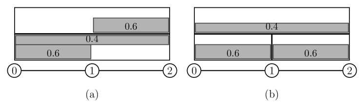
Figure 1: Two optimum solutions of an instance of the stationary problem on a linear array network with $n=3$ nodes

It is customary to consider two problem variations: non-splittable, in which a transmission must be assigned to a single light-trail, and splittable, in which a transmission can be split into two or more transmissions by dividing up the bandwidth requirement, and each of them can be assigned to different light-trails. Note that when a transmission is split into multiple transmissions, the length and extent remains same, only the height is divided. Our results hold for both variations.

Note that the Bin Packing problem which is NP-hard, is a special case of the stationary problem where each item corresponds to a transmission from node $0$ to node $n-1$ and each bin corresponds to a light-trail (and to a wavelength too because each light-trail completely occupies a wavelength). Thus the non-splittable stationary problem is NP-hard. We do not know whether the splittable problem is also NP-hard.

We will use $c_{l}(S)$ to denote the congestion induced on a link $l$ by a set $S$ of transmissions. This is simply the total bandwidth requirement of those transmissions from $S$ requiring to cross link $l$. Clearly $c(S)=\max_{l}c_{l}(S)$, the maximum congestion over all links, is a lower bound on the number of wavelengths needed. Finally if $t$ is a transmission, then we abuse notation to write $c_{l}(t),c(t)$, instead of $c_{l}(\{t\}),c(\{t\})$, for the congestion contributed by $t$ only, which is equal to the bandwidth requirement of $t$. Let $R$ be the set of all transmissions of an instance of the stationary problem. We will use $c$ to denote the overall congestion $c(R)$.

3.1 Algorithm Overview

Getting an algorithm which requires only $O(c\log n)$ wavelengths is easy. If $c_{n/2}$ denotes the congestion of the link between node $n/2$ and node $n/2+1$, then the transmissions crossing this link can be scheduled in $\left\lceil c\right\rceil\geq\left\lceil c_{n/2}\right\rceil$ wavelengths for the splittable case, and twice that many for the non-splittable case (using ideas from Bin Packing [47]). The remaining transmissions do not cross the middle link, and hence can be scheduled by separately solving two subproblems, one for the transmissions on each half of the array. The two subproblems can share the wavelengths. If $\lambda(n,c)$ denotes the number of wavelengths used for scheduling transmissions of congestion at most $c$ in a linear array of $n$ nodes, we have the recurrence $\lambda(n,c)=O(\left\lceil c\right\rceil)+\lambda(c,n/2)$. Clearly this solves to $O(c\log{n})$. Getting a solution using $O(c+\log{n})$ wavelengths requires a different divide and conquer approach.

The first observation behind our algorithm is that it is relatively easy to get a good schedule if all the transmissions had the same length (see Section 3.2). So we divide the transmissions into classes based on their lengths, then schedule each class separately and finally merge the schedules. Naively scheduling and merging each class would give us an $O(c\log{n})$ wavelength algorithm; with some care we do get the required $O(c+\log{n})$ wavelength algorithm. Our algorithm is:

1. Partition into classes. Say a transmission belongs to class $i$ if its length is between $2^{i-1}$ (exclusive) and $2^{i}$ (inclusive). Let $R_{i}$ denote the set of transmissions of class $i$, for $i=0$ to $\left\lceil\log_{2}(n-1)\right\rceil$.

2. Schedule transmissions of each class separately. It will be seen that each class can be scheduled efficiently, i.e. using $O(1+c(R_{i}))$ wavelengths.

3. Merge the schedules of different classes. We do not simply collect together the schedules constructed for the different classes, but do need to mix them together, as will be seen.

Scheduling classes $R_{0},R_{1}$ is easy. Note that each transmission in $R_{0}$ has length $1$. So they can be assigned to light-trails created by simply putting shutters OFF at every node on all the wavelengths that are to be used. Now for a fixed $l$ consider the light-trails $[l,l+1]$ on all the wavelengths. Each of these light-trails can be thought of as a bin in which the transmissions $[l,l+1]$ are to be assigned. Clearly, $\left\lceil c_{l}(R_{0})\right\rceil$ light-trails will suffice for the splittable case, and twice that many for the non-splittable case (using ideas from Bin Packing [47]). Since the light-trails for different $l$ do not overlap, they can be on the same wavelength. So $\max_{l}O(\left\lceil c_{l}(R_{0})\right\rceil)=O(\left\lceil c(R_{0})\right\rceil)$ wavelengths will suffice. Transmissions in $R_{1}$ have length $2$. So they can be assigned to light-trails created on two sets of wavelengths – one having shutters OFF at even nodes and the other having shutters OFF at odd nodes. Transmissions starting at an even (odd) node are assigned to a light-trail on a wavelength of the first (second) set. Using a argument similar for the transmissions in $R_{0}$, we can show that each of these sets require $O(\left\lceil c(R_{1})\right\rceil)$ wavelengths. So for the rest of this paper we only consider classes $2$ and larger.

3.2 Schedule Class $i\geq 2$

It seems reasonable that if the class $R_{i}$ is further split into subclasses each of which has $O(1)$ congestion, then the subclasses could be scheduled using $O(1)$ wavelengths. This intuition is incorrect for an arbitrary collection of transmissions with congestion $O(1)$, as will be seen in Section 4. However, the intuition is correct when the transmissions have nearly the same length, as they do when taken from any single $R_{i}$.

Lemma 1.

There exists a polynomial time procedure to partition $R_{i}$ into sets $S_{1},S_{2},\ldots,S_{k}$ where $k\leq\left\lceil c(R_{i})\right\rceil$ such that (i) $c(S_{j})<4$ for all $j$, and (ii) if a transmission in $S_{j}$ uses link $l$ then $\left\lceil c_{l}(R_{i})\right\rceil\geq j$.

Proof.

We start with $T_{1}=R_{i}$, and in general given $T_{j}$ we pick a subset of transmission $S_{j}$ from $T_{j}$ using a procedure described below and repeat with the remaining transmissions $T_{j+1}=T_{j}\setminus S_{j}$ until $T_{j+1}$ becomes empty for some value $k$ of $j$.

For each link $l$ from left to right, we greedily pick transmissions crossing link $l$ into $S_{j}$ until we have removed at least unit congestion from $c_{l}(T_{j})$ or reduced $c_{l}(T_{j})$ to 0. Note that if the transmissions already picked while considering the links on the left of $l$ also have congestion at least $1$ at link $l$ then we do not add any more transmission while considering link $l$. So at the end the following condition holds:

$$\forall l,\,c_{l}(S_{j})\left\{\begin{array}[]{ll}=c_{l}(T_{j})&\text{if}\;c_{l}(T_{j})\leq 1,\;\text{and}\\ \geq 1&\text{otherwise.}\end{array}\right.$$ (1)

However, to make sure that $c(S_{j})$ is not large, we move back transmissions from $S_{j}$, in the reverse order as they were added, into $T_{j}$ so long as condition (1) remains satisfied. It can be seen that the construction of $S_{j}$ takes at most $n|T_{j}|$ time in the pick-up step and also in the move-back step.

Now we show that condition (i) of the lemma is satisfied, i.e., $c(S_{j})<4$ for all $j$. At the end of move-back step, for any transmission $t\in S_{j}$ there must exist a link $l$ such that $c_{l}(S_{j})<1+c(t)$ otherwise $t$ would have been removed. We call $l$ as a sweet spot for $t$. Since $c(t)\leq 1$ we have $c_{l}(S_{j})<2$ for any sweet spot $l$.

Now consider any link $x$. Of the transmissions through $x$, let $L_{1}$ ($L_{2}$) denote transmissions having their sweet spot on the left (right) of $x$. Consider $y$, the rightmost of these sweet spots of some transmission $t\in L_{1}$. Note first that $c_{y}(S_{j})<2$. Also all transmissions in $L_{1}$ pass through both $x,y$. Thus $c_{x}(L_{1})=c_{y}(L_{1})\leq c_{y}(S_{j})<2$. Similarly, $c_{x}(L_{2})<2$. Thus $c_{x}(S_{j})=c_{x}(L_{1})+c_{x}(L_{2})<4$. But since this applies to all links $x$, $c(S_{j})<4$.

To show that the condition (ii) is also satisfied, suppose $S_{j}$ contains a transmission that uses some link $l$. The construction process above must have removed at least unit congestion from $l$ in every previous step $1$ through $j-1$. Thus $c_{l}(R_{i})>j-1$. That implies $\left\lceil c_{l}(R_{i})\right\rceil\geq j$. This also implies that $k\leq\max_{l}\left\lceil c_{l}(R_{i})\right\rceil=\left\lceil c(R_{i})\right\rceil$. ∎

A transmission $t$ is said to cross a node $u$ if $t$ starts at a node on the left of $u$ and ends at a node on the right of $u$. Since every transmission $t$ in $S_{j}$ has length at least $2^{i-1}+1$, $t$ must cross some node whose number is a multiple of $2^{i-1}$. The smallest numbered such node is called the anchor of $t$. The trail-point of a transmission $t$ is the right most node numbered with a multiple of $2^{i-1}$ that is on the left of the anchor of $t$. If the transmission has trail-point at node $q2^{i-1}$ for some $q$, then we define $q\bmod 4$ as its phase.

Lemma 2.

The set $S_{j}$ can be scheduled using $O(1)$ wavelengths.

Proof.

We partition $S_{j}$ further into sets $S_{j}^{p}$ containing transmissions of phase $p$. Note that the transmissions in any $S_{j}^{p}$ either overlap at their anchors, or do not overlap at all. This is because if two transmissions in $S_{j}^{p}$ have different anchors, then these two anchors are at least $2^{i+1}$ distance apart. Since the length of each transmission is at most $2^{i}$, the two transmissions can not intersect.

So for the set $S_{j}^{p}$, consider $4$ wavelengths, each having shutters OFF at nodes numbered $(4q+p)2^{i-1}$. Let $x=(4q+p)2^{i-1}$ and $y=(4(q+1)+p)2^{i-1}=x+2^{i+1}$ be two nearest node having shutters OFF. Among the light-trails thus created, for a fixed $q$, each of the $4$ light-trails $[x,y]$ can be thought of as a bin in which the transmissions having extent totally within $[x,y]$ and total bandwidth requirement at most 1 are to be assigned. This is an instance of the Bin Packing problem. Clearly, for a fixed $q$, these $4$ light-trails will suffice for the splittable case, because $c(S_{j}^{p})<4$. Since the light-trails for different $q$ do not overlap, the instances of the Bin Packing problem can share wavelengths and hence these $4$ wavelengths will suffice. For the non-splittable case, $8$ wavelengths will suffice, using standard Bin Packing ideas, e.g., First-Fit [47].

Thus all of $S_{j}$ can be accommodated in at most $16$ wavelengths for the splittable case, and at most $32$ wavelengths for the non-splittable case. ∎

Lemma 3.

The entire set $R_{i}$ can be scheduled such that at each link $l$ there are $O(C_{l}(R_{i})+1)$ light-trails.

Proof.

We first consider the light-trails as constructed in Lemma 2. In this construction, uniformly at all links there are at most $\left\lceil c(R_{i})\right\rceil\leq c(R_{i})+1$ sets of light-trails such that each set corresponds to $O(1)$ light-trails created to schedule the transmissions of an $S_{j}$. Note that $c(R_{i})=\max_{l}c_{l}(R_{i})$. So, in this construction the condition of the lemma is surely satisfied for the link where the congestion is maximum. For other links the condition of the lemma may not be satisfied because (1) there may be empty light-trails and (2) some light-trails may contain links that are not used by any of the transmissions associated with the light-trail. So we remove empty light-trails and in case (2) we shrink the light-trails by removing the unused links (which can only be near either end of the light-trail because all transmissions assigned to a light-trail overlap at their anchor). We prove next that with this modification, the condition of the lemma is satisfied.

Let $j$ be the largest such that a transmission from $S_{j}$ uses link $l$. After the modification the light-trails that carries transmissions from $S_{j^{\prime}}$ for $j^{\prime}>j$ do not use link $l$. So now there are $j$ sets of light-trails using link $l$ such that each set has $O(1)$ light-trails. However we know from Lemma 1 that $j\leq\left\lceil c_{l}(R_{i})\right\rceil\leq c_{l}(R_{i})+1$. Thus there are a total of $O(j)=O(c_{l}(R_{i})+1)$ light-trails at link $l$. ∎

3.3 Merge Schedules of All Classes

If we simply collect together the wavelengths as allocated above, we would get a bound $O(c\log n)$. Note however, that if two light-trails, one for transmissions in class $i$ and the other for transmissions in class $j$, are spatially disjoint, then they could possibly share the same wavelength. Given below is a systematic way of doing this, which gets us a sharper bound.

Theorem 4.

The entire set $R$ can be scheduled using $O(c+\log n)$ wavelengths.

Proof.

We know that after the modification in Lemma 3, at each link $l$ there are a total of $O(c_{l}(R_{i})+1)$ light-trails for each class $i$. Thus summing over all classes, the total number of light-trails at $l$ are $O(c_{l}(R)+\log n)$.

Think of each light-trail as an interval, giving us a collection of intervals such that any link $l$ has at most $O(c_{l}(R)+\log n)=O(c+\log{n})$ intervals. Now this collection of intervals can be colored using $O(c+\log{n})$ colors [48]. Now for each color $w$, use a separate wavelength and configure the light-trails corresponding to the intervals of color $w$ by setting the shutters OFF at the nodes corresponding to the endpoints of the intervals. Hence $O(c+\log n)$ wavelengths suffice. ∎

4 On the Congestion Lower Bound

We now consider an instance of the stationary problem. For convenience, we assume there are $n+1$ nodes numbered $0,\ldots,n$ where $n=2^{k}$ for some $k$ and all logarithms are with base $2$. All the transmissions have same bandwidth requirement $b=1/(\log n+1)$.

First, we have a transmission going from $0$ to $n$. Then a transmission from $0$ to $n/2$ and a transmission from $n/2$ to $n$. Then four transmissions spanning one-fourth the distance, and so on. Thus we have transmissions of $\log n+1$ classes, each class having transmissions of same length. In class $i\in\{0,1,\ldots,\log n\}$ there are $n/2^{i}$ transmissions $B(s_{ij},d_{ij})=b$ where $s_{ij}=j2^{i},d_{ij}=(j+1)2^{i}$ for all $j=0,1,\ldots,(n/2^{i})-1$. All other entries of $B$ are $0$. This is illustrated in Fig. 2(a) for $n=17$.

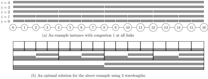
Figure 2: An example instance where congestion bound is weak

Clearly the congestion of this pattern is uniformly $1$. Our algorithm will use $\log n+1$ wavelengths, each serving all transmissions of a single class.

Consider an optimal solution for the non-splittable case. There has to be a light-trail in which the transmission $[0,n]$ is scheduled. Thus we must have a wavelength with no OFF shutters except at node 0 and node $n$. In this wavelength, it is easily seen that the longest transmissions should be scheduled. So we start assigning transmissions of first few classes in this light-trail. Suppose, all the transmissions for first $l$ classes are assigned. Then we have total $1+2+4+\cdots+2^{l}=2^{l+1}-1$ transmissions assigned to this light-trail. Total bandwidth requirement of these transmissions should be at most 1. This gives us $(2^{l+1}-1)(1/(\log n+1))\leq 1$ implying $l\leq\log(\log n+2)-1\approx\log\log n$.

For the subsequent classes of transmissions, we allocate a new wavelength and create light-trails by putting shutters OFF at nodes $qn/2^{l+1}$ for all possible $q$. It can be seen that again transmissions of next about $\log\log n$ classes can be put in these light-trails. We repeat this process until all transmissions are assigned.

In each wavelength we assign transmissions of $\log\log n$ classes. There are total $(1+\log n)$ classes. Thus the total number of wavelengths needed is $\lceil(1+\log n)/\log\log n\rceil=\Omega(\log{n}/\log\log{n})$ rather than the congestion bound of $1$.

For the example in Fig. 2(a), using this procedure, we have $\log\log n=2$. Thus we require $\lceil(1+\log n)/\log\log n\rceil=3$ wavelengths. The first wavelength is used for the transmissions of classes $\{3,4\}$, the second wavelength for classes $\{1,2\}$ and the third for class $0$. This solution is shown in Fig. 2(b).

Suppose we add $c-1$ transmissions of extent $[0,n]$ and bandwidth requirement $1$ to this pattern of transmissions of congestion $1$ uniformly at all links. We can similarly show that an optimal solution will require $c-1+\Omega(\log{n}/\log\log{n})$ wavelengths. Thus we will get an instance of congestion $c$ uniformly at all links but which requires $\Omega(c+\log{n}/\log\log{n})$ wavelengths, for any $c$.

5 The On-line Problem

In the on-line case, the transmissions arrive dynamically. An arrival event has parameters $(s_{i},d_{i},r_{i})$ respectively giving the origin, destination, and bandwidth requirement of an arriving transmission request. The algorithm must assign such a transmission to a light-trail $L$ such that $s_{i},d_{i}$ belong to the light-trail, and at any time the total bandwidth requirement of transmissions assigned to any light-trail is at most $1$. A departure event marks the completion of a previously scheduled transmission. The corresponding bandwidth is released and becomes available for future transmissions. The algorithm must make assignments without knowing about subsequent events.

Unlike the stationary problem, congestion at any link may change over time. Let $c_{lt}(S)$ denote the congestion induced on a link $l$ at time $t$ by a set of transmissions $S$. This is simply the total bandwidth requirement of those transmissions from $S$ requiring to cross link $l$ at time $t$. The congestion lower bound $c(S)$ is $\max_{l}\max_{t}c_{lt}(S)$, the maximum congestion over all links over all time instants.

For the on-line problem, we present two algorithms – (1) SeparateClass having competitive ratio $\Theta(\log{n})$ and (2) AllClass, a simplification of SeparateClass inspired by the analysis of the algorithm for the stationary problem, as may be seen. However, we show that this simplification not necessarily makes it better. In fact we show that AllClass has competitive ratio in between $\Omega(\log^{2}n/\log\log n)$ and $O(\log^{2}{n})$.

Now we present our two on-line algorithms. In both the on-line algorithms, when a transmission request arrives, we first determine its class $i$ and trail-point $x$ (defined in Section 3.2). The transmission is allocated to some light-trail $[x,x+2^{i+1}]$. However, the algorithms differ in the way a light-trail is configured on some candidate wavelength.

5.1 Algorithm SeparateClass

In this algorithm, every allocated wavelength is assigned a class label $i$ and a phase label $p$, and has shutters OFF at nodes $(4q+p)2^{i-1}$ for all $q$, i.e., is configured to serve only transmissions of class $i$ and phase $p$. Whenever a transmission $t$ of class $i$ and phase $p$ is to be served, it is only served by a wavelength with the same labels. If such a wavelength $w$ is found, and a light-trail $L$ on $w$ starting at the trail-point of $t$ has space, then $t$ is assigned to the light-trail $L$. If no such wavelength is found, then a new wavelength $w^{\prime}$ is allocated, it is labeled and configured for class $i$ and phase $p$ as above and $t$ is assigned to the light-trail on $w^{\prime}$ that starts at the trail-point of $t$.

When a transmission finishes, it is removed from its associated light-trail. When all transmissions in a wavelength finish, then its labels are removed, and it can subsequently be used for other classes or phases.

Lemma 5.

Suppose, at some instant of time, among the wavelengths allocated by SeparateClass, $x$ wavelengths had non-empty light-trails of the same class and phase across a link $l^{\prime}$. Then there must be a link $l$ having congestion $\Omega(x)$ at some instant of time.

Proof.

Suppose at some instant of time, wavelengths $w_{1},w_{2},\ldots,w_{x}$, ordered according to the time of allocation, had non-empty light-trails $L_{1},L_{2},\ldots,L_{x}$, respectively, of same class and phase across link $l^{\prime}$. Let $u$ be the anchor (defined in Section 3.2) of the transmissions assigned on these light-trails and $l$ be the link between node $u$ and node $u+1$.

Now suppose wavelength $w_{x}$ was allocated due to a transmission $t$. This could only happen because $t$ could not fit in the wavelengths $w_{j}$ for all $j\leq x-1$.

For the splittable case this can only happen if light-trails $L_{1}$ through $L_{x-1}$ together contain transmissions of congestion at least $x-1-c(t)=\Omega(x)$ crossing the anchor $u$ of $t$, when $t$ arrived. Thus at that time $l$ had congestion $\Omega(x)$, giving us the result.

For the non-splittable case, suppose that $c(t)\leq 0.5$. Then the transmissions in each of the light-trails $L_{j},1\leq j\leq x-1$, must have congestion of least $0.5$ at $l$ when $t$ arrived, giving congestion $\Omega(x)$. So suppose $c(t)>0.5$. Let $k$ be the largest such that light-trail $L_{k}$ contains a transmission $t^{\prime}$ with $c(t^{\prime})\leq 0.5$ when $t$ arrived. If no such $k$ exists, then clearly the congestion at $l$ when $t$ arrived is $\Omega(x)$. If $k$ exists, then all the light-trails $L_{j}$, $j>k$ have transmissions of congestion at least $0.5$ at $l$ when $t$ arrived. And the light-trails $L_{j}$, $j\leq k$ had transmissions of congestion at least $0.5$ at $l$ when $t^{\prime}$ arrived. So at one of the two time instants the congestion at $l$ must have been $\Omega(x)$. ∎

Theorem 6.

SeparateClass is $\Theta(\log n)$ competitive.

Proof.

Suppose that SeparateClass uses $w$ wavelengths. We will show that the best possible algorithm (including off-line algorithms) must use at least $\Omega(w/\log{n})$ wavelengths. That will prove that SeparateClass is $O(\log n)$ competitive.

Consider the time at which the $w$th wavelength was allocated. At this time $w-1$ wavelengths are already in use, and of these at least $w^{\prime}=(w-1)/(4\log{n})$ must have the same class and phase. Among these $w^{\prime}$ wavelengths consider the one which was allocated last to accommodate some light-trail $L$ serving some newly arrived transmission. At that time, each of the previously allocated $w^{\prime}-1$ wavelengths was nonempty in the extent of $L$. By Lemma 5, there is a link that had congestion $\Omega(w^{\prime}-1)=\Omega(((w-1)/(4\log{n}))-1)=\Omega(w/\log{n})$ at some time instant. This is a lower bound on any algorithm, even off-line.

We show the lower bound $\Omega(\log n)$ using the following example. Let $n=2^{k}+1$. At each time $t=0,1,\ldots,k$, a transmission $[0,2^{t}]$ arrives. All transmissions have bandwidth requirement $1/(k+1)$. At time $k+1$ all transmissions depart together. SeparateClass takes $k$ wavelengths because each transmission is of a different class. The optimal off-line algorithm assigns all of them to a single light-trail spanning the complete network and hence takes only one wavelength. ∎

5.2 Algorithm AllClass

This is a simplification of SeparateClass in that the allocated wavelengths are not labeled. When a transmission $t$ of class $i$ and trail-point $x$ arrives, we search the wavelengths in the order they were allocated for a light-trail $L$ of extent $[x,x+2^{i+1}]$ such that $L$ has enough space to serve $t$. If such a light-trail $L$ is found, then $t$ is assigned to $L$. If no such light-trail is found, then an attempt is made to create a light-trail $[x,x+2^{i+1}]$ from the unused portions of one of the existing wavelengths in a first-fit manner in the order they were allocated. If such a light-trail $L$ can be created, then $L$ is created and $t$ is assigned to $L$. Otherwise a new wavelength $w$ is allocated, the required light-trail $L$ of extent $[x,x+2^{i+1}]$ is created on $w$, and $t$ is assigned to $L$. The portion of the wavelength $w$ outside the extent of $L$ is marked unused.

When a transmission finishes, it is removed from its associated light-trail. If this makes the light-trail empty then we mark its extent on the corresponding wavelength as unused.

Theorem 7.

AllClass is $O(\log^{2}n)$ competitive.

Proof.

Suppose AllClass uses $w$ wavelengths. We will show that an optimal algorithm will use at least $\Omega(w/\log^{2}n)$. Clearly, we may assume $w=\Omega(\log^{2}n)$.

We first prove that there must exist a point of time in the execution of AllClass when there are at least $w/(4\log{n})$ non-empty light-trails (not necessarily of same class and phase) crossing the same link.

Number the wavelengths in the order of allocation. Consider the transmission $t$ for which the $w$th wavelength was allocated for the first time. Let $L$ be the light-trail used for $t$. Clearly, the $w$th wavelength had to be allocated because at that time the $w-1$ previously allocated wavelengths contained light-trails overlapping with $L$. Let $S^{\prime}$ denote this set of light-trails overlapping with $L$. A light-trail $L^{\prime}\in S^{\prime}$ can be any of the three types - (1) $L$ and $L^{\prime}$ overlap at the leftmost link of $L$, (2) $L$ and $L^{\prime}$ overlap at the rightmost link of $L$ but not at the leftmost link of $L$, and (3) $L^{\prime}$ is totally contained in the extent of $L$, without containing either the leftmost or the rightmost link of $L$. Construct $S\subseteq S^{\prime}$ having exactly one light-trail from each of the $w-1$ wavelengths by picking light-trails from $S^{\prime}$ in the order – first of type 1, then of type 2 and finally of type 3. Now we consider three possible cases.

Case 1: $S$ has at least $w/(4\log{n})$ light-trails of type 1. Then we have $w/(4\log{n})$ light-trails crossing the leftmost link of $L$.

Case 2: $S$ has at least $w/(4\log{n})$ light-trails of type 2. Then we have $w/(4\log{n})$ light-trails crossing the rightmost link of $L$.

Case 3: $S$ has less than $w/(4\log{n})$ light-trails of type 1 and less than $w/(4\log{n})$ light-trails of type 2. Then, number of light-trails of type 3 in $S$ must be at least $w^{\prime}=w-1-2w/(4\log{n})=w-1-w/(2\log{n})$. Let $L^{\prime}\in S$ be the light-trail allocated on the $w^{\prime}$th of the wavelengths having a light-trail of type 3 in $S$. Note that $L^{\prime}$ is strictly smaller than $L$. Thus we can repeat the above argument by using $L^{\prime}$ and $w^{\prime}$ in place of $L$ and $w$ respectively, only $\log{n}$ times, and if we fail each time to find at least $w/(4\log{n})$ light-trails crossing a link, we will end up with a light-trail $L^{\prime\prime}$ such that there are at least $w^{\prime\prime}$ wavelengths having light-trails conflicting with $L^{\prime\prime}$, where $w^{\prime\prime}=w-\log{n}-\log{n}(w/(2\log{n}))=w/2-\log{n}\geq w/(4\log{n})$ for $w=\Omega(\log^{2}n)$. But $L^{\prime\prime}$ is a single link and so we are done.

Of these $w/(4\log{n})$ light-trails, at least $w/(16\log^{2}n)$ must have the same class and phase. But it can be shown that Lemma 5 is also true for AllClass, and hence there is a link having congestion $\Omega(w/(16\log^{2}n))$ at some time instant. But this is a lower bound on the number of wavelengths required by any algorithm, including an off-line algorithm. ∎

5.3 Lower Bound for AllClass

We give a sequence of transmissions for which AllClass takes $\Omega(\log^{2}n/\log\log n)$ wavelengths but an optimal off-line algorithm, Opt, requires only one wavelength.

Theorem 8.

AllClass is $\Omega(\log^{2}n/\log\log n)$ competitive.

Our transmission sequence consists of several (exact count will be shown later) subsequences, which we call stages. In all stages, all transmissions have height, i.e., bandwidth requirement of $1/n^{2}$. Our transmission sequence is such that, at any point of time, there are less than $n^{2}$ active transmissions. Opt will put all transmissions in a single light-trail using full length of a wavelength. On the other hand, it will be seen that AllClass will allocate $\Omega(\log^{2}n/\log\log n)$ wavelengths in total for all stages. We describe the first stage only, the other stages are scaled versions of the first stage. The goal of the first stage is to force AllClass to allocate wavelengths with light-trail patterns given in the following lemma.

Lemma 9.

Let the network have $q+1$ nodes numbered $0,\ldots,q$. Then there is a transmission sequence for which AllClass allocates $k=\left\lfloor\log q\right\rfloor$ wavelengths numbered $0,\ldots,k-1$, with the following pattern $P$ of light-trails: each wavelength $i$ has $\left\lfloor n/k\right\rfloor$ unit-length light-trails $[jk+i,jk+i+1]$, each containing a single transmission, for all $j=0,\ldots,\left\lfloor n/k\right\rfloor-1$.

Proof.

For simplicity we assume $q=2^{k}$, i.e., $k$ is exactly equal to $\log q$. The general case can be similarly proved.

Note that the pattern $P$ has non-overlapping and unit-length light-trails. We first describe how to create a unit-length light-trail $[x,x+1]$ on any wavelength $i$. We will repeatedly use this procedure to create the pattern $P$. For this purpose, we define $Hill(h,x)$ to be an ordered sequence of $h$ transmissions as follows. For each $i=0,1,\ldots,h-1$, $Hill(h,x)$ contains a transmission that uses the link $[x,x+1]$ and has class $k-1-i$, and some suitable phase. The key point is that all the transmissions in a hill overlap but have different classes, and hence AllClass must assign them in distinct light-trails on different wavelengths. Thus starting from scratch, the arrival of the transmissions in a hill will cause $h$ wavelengths to be allocated. For example, we show $Hill(h=4,31)$ on right half of Fig. 3LABEL:sub@parta. Further, if a new transmission $[x,x+1]$ arrives, it will cause one more wavelength to be allocated. From now on, by creating (deleting) a hill we mean the arrival (departure) of transmissions in a hill.

Now we describe how to generate the pattern $P$ using several hills. The idea is to build the portion of the pattern on one wavelength at a time from top to bottom, i.e., first create all light-trails of $P$ on wavelength $k-1$, then all light-trails on wavelength $k-2$ and so on. Each unit-length light-trail $[x,x+1]$ on an wavelength is created by temporarily creating an appropriate hill underneath it, then creating the transmission $[x,x+1]$ and finally deleting the temporary hill. However, to make sure that all the wavelengths numbered $0,\ldots,k-2$ that were allocated when the part of the pattern on wavelength $k-1$ was created, remain alive throughout, we use the following trick. We create left half of $P$ first. Then we create the right half.

Before creating the left half, we first create hill $H=Hill(k-1,q-1)$. This hill will survive until the left half is completely created. Its sole purpose is to keep $k-1$ wavelengths alive. The left half is created top to bottom as given in Algorithm 1. Consider the first execution of the insertion marked as belonging to $P$. Because of the hill $H^{\prime}$, this transmission will clearly be assigned to a light-trail on wavelength $i$. Note further that when transmissions in $H^{\prime}$ depart, the wavelengths $0,\ldots,i-1$ do not become empty because of the presence of hill $H$ in the right half. Thus the subsequent iterations also force the transmissions to be assigned in wavelength $i$, and so on.

  for $i=k-1$ downto 0 do

     for $j=0$ to $q/2k$ do

        Create a hill $H^{\prime}=Hill(i,jk+i)$

        Insert an arrival event for transmission $[jk+i,jk+i+1]$ {belongs to $P$}

        Remove hill $H^{\prime}$

     end for

  end for

Algorithm 1 Create left half of $P$

At the end of the above, we will have created a pattern as shown in Fig. 3LABEL:sub@parta. Since each light-trail contains only one transmission, we just show the transmissions instead of the light-trails.

Next we remove $H$, and execute the same code to create the right half of $P$ on the $k$ wavelengths already allocated. Note that the light-trails created in the left half now serve the purpose that $H$ did earlier. At this point we will have the complete pattern $P$. ∎

The first stage is created by using Lemma 9 with $q=n$. In the second stage, we can treat every $k=\left\lfloor\log n\right\rfloor$ nodes as a single node, and think of the network as having $n^{\prime}=\left\lfloor n/k\right\rfloor$ nodes. We create a pattern of height $\left\lfloor\log{n^{\prime}}\right\rfloor$ similar to $P$ but with light-trails of length $k$ using Lemma 9 with $q=n^{\prime}$. Since these light-trails are longer than the light-trails in the previous stage, we can stack up the new pattern on the top of the previous pattern. We can keep doing this until $n^{\prime}$ becomes less than $2$. It can be shown that the number of stages is $\Omega(\log_{\log n}n)=\Omega(\log n/\log\log n)$.

Let $T(n)$ denote the total height of the patterns thus created for $n+1$ nodes, then $T(n)$ is computed using the following recurrence:

$$T(n)=\left\lfloor\log n\right\rfloor+T(\left\lfloor n/\left\lfloor\log n\right\rfloor\right\rfloor)\qquad\text{or simply}\qquad T(n)=\log n+T(n/\log n)$$ (2)

with the base condition $T(n)=0$ for $n\leq 1$. It can be shown that the recurrence has solution $T(n)=\Omega(\log^{2}n/\log\log n)$.

Thus AllClass will use $\Omega(\log^{2}n/\log\log n)$ wavelengths for the patterns created. Fig. 3LABEL:sub@partb shows all the transmissions active at the end of all stages, for the example considered in Fig. 3LABEL:sub@parta.

(a)

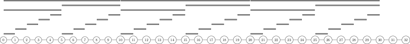
(b)

Figure 3: An instance for which AllClass is $\Omega(\log^{2}n/\log\log n)$ competitive

5.4 Remarks

It is interesting to note that AllClass is more flexible than SeparateClass, and it is this flexibility that is exploited in the lower bound argument to show a worse ratio for AllClass than SeparateClass.

Indeed, the more flexibility we give, the worse it seems the ratio will become. In AllClass, if we have a transmission of length $L=2^{k}$ we assign it to a light-trail of length $2L$. This seems wasteful. But this is done to accommodate transmissions that do not start at a multiple of $L/4$, using only $4$ phases. Suppose we decide to be more flexible, and allow light-trails to start anywhere (so long as their length is $2^{k}$ for some $k$) using $2^{k}$ phases. Although this strategy will handle the above transmission better, in general it is worse in that its competitive ratio can be shown to be $\Omega(\log^{2}n)$. We omit the details.

6 Problem Lower Bound – $\Omega(\log n)$

Let Alg be some algorithm for the on-line problem and Opt be an optimal off-line algorithm. By observing the behaviour of Alg we can create a sequence of transmissions for which Alg takes $\Omega(\log{n})$ times as many wavelengths as Opt. This gives us the lower bound.

Theorem 10.

There exists a transmission sequence for which any on-line algorithm requires $\Omega(\log{n})$ times as many wavelengths as the optimal off-line algorithm.

For convenience we assume that the network has $n+1$ nodes numbered $0,1,\ldots,n$ and $n=2^{k}$ for some $k$. The transmission sequence we use to prove Theorem 10 is made of $k=\log n$ stages. For stage $i=0,1,\ldots,k-1$, consider the network broken up into $n^{\prime}=n/l$ intervals of length $l=2^{i}$. Let this set of intervals be $Q_{i}=\{[ql,(q+1)l]\}_{q=0}^{n^{\prime}-1}$. At the beginning of the $i$th stage, for each interval $I\in Q_{i}$, $k^{2}$ transmissions having extent $I$ arrive. We will denote this set of $n^{\prime}k^{2}$ transmissions by $A_{i}$. All transmissions have height (i.e., bandwidth requirement) of $1/k$. At the end of the $i$th stage, all but a subset $S_{i}$ of $A_{i}$ depart. The set $S_{i}$ is found with properties as per the following Lemma.

Lemma 11.

Among the $n^{\prime}k^{2}$ transmissions arriving at the beginning of stage $i$, we can find a set $S_{i}$ of $n^{\prime}k$ transmissions such that (1) Exactly $k$ transmissions from $S_{i}$ are for a single interval $I\in Q_{i}$, (2) Alg assigns each transmission in $S_{i}$ to a distinct light-trail.

Proof.

We have $k^{2}$ transmissions for each interval $I\in Q_{i}$. Partition these $k^{2}$ transmissions arbitrarily into $k$ groups of $k$ transmissions each. So overall we have $n^{\prime}k$ groups each containing $k$ transmissions. Now form a bipartite graph $(U,V,E)$ as follows.

1. $U$ has $n^{\prime}k$ vertices, each vertex corresponding to a group of $k$ transmissions as formed above. Note that there are $k$ groups for each interval, and hence we can consider a distinct group of $k$ vertices of $U$ to be associated with each $I\in Q_{i}$.

2. $V$ has a vertex corresponding to each light-trail used by Alg for serving the transmissions of this stage.

3. $E$ has following edges. Suppose a transmission $t$ from the group associated with a vertex $u\in U$ is placed by Alg in the light-trail $L$ associated with a vertex $v\in V$. Then for each such $t$ there will be an edge $(u,v)$ in $E$. Note that this may produce parallel edges if several transmissions in the group of $u$ are placed in $L$.

The degree of each vertex in $U$ is exactly $k$, one edge for each transmission in the associated group. Consider any vertex $v\in V$. Since its associated light-trail can accommodate at most $k$ transmissions of height $1/k$, its degree must be at most $k$.

Now consider any subset $S$ of vertices from $U$ and its neighborhood $T$ in $V$. Because vertices in $U$ have degree exactly $k$ there must be exactly $|S|k$ edges leaving $S$. These must be a subset of the edges entering $T$. But vertices in $V$ have degree at most $k$. So there can be at most $|T|k$ edges entering $T$. Thus we have $|S|k\leq|T|k$, i.e., $|T|\geq|S|$, i.e., $S$ has at least as many neighbors as its own cardinality. But this is true for any $S$. Thus by the generalization of Hall’s theorem, there must be a matching $M$ that includes an edge from every vertex of $U$ to a distinct vertex in $V$.

Consider the set $S_{i}$ of transmissions associated with each edge of $M$. Since there is exactly one edge in $M$ for each node in $U$, $S_{i}$ has one transmission per group of transmissions for each interval. Hence $S_{i}$ has exactly $k$ transmissions for each interval. Since $M$ has exactly one edge per vertex in $V$, we know that each transmission in $S_{i}$ is assigned to a distinct light-trail by Alg. ∎

We have now completely described the transmission sequence. At the end all transmissions have departed except those in some $S_{i}$. We will use $D_{i}$ to denote the transmissions which depart in stage $i$. Clearly $A_{i}=S_{i}\cup D_{i}$.

Lemma 12.

Opt uses overall $2k-1$ wavelengths while processing the transmission sequence for all stages.

Proof.

Consider stage $i$. The set $A_{i}$ has $k^{2}$ transmissions for each interval $I\in Q_{i}$. To serve these transmissions $A_{i}$, Opt uses $k$ wavelengths configured as follows. Each wavelength is configured into light-trails as per $Q_{i}$, i.e., each interval $I\in Q_{i}$ forms one light-trail. Now the key point is that Opt places all transmissions in $S_{i}$ into light-trails on a single wavelength. This can be done because the set $S_{i}$ indeed has $k$ transmissions for each $I\in Q_{i}$. The remaining transmissions $D_{i}$ can be accommodated into $k-1$ additional wavelengths. Note now that at the end of the stage, the transmissions $D_{i}$ depart. Hence although the stage used $k$ wavelengths transiently, at the end $k-1$ of these are released.

Thus, at the end of stage $i$, there will be $i+1$ wavelengths in use, one for transmissions in each $S_{j}$, $j=0,\ldots,i$. When $A_{i+1}$ arrives, Opt will allocate $k$ new wavelengths. So while processing $A_{i+1}$ there will be $i+1+k$ wavelengths in use. These will drop down to $i+2$ at the end of stage $i+1$. Thus, over all the stages the maximum number of wavelengths used will be at most $\max_{i=0,\ldots,k-1}(i+k)$, i.e. $2k-1$. ∎

Lemma 13.

Alg uses at least $k^{2}/2$ wavelengths while processing the transmission sequence.

Proof.

Consider the light-trails used by Alg which are active at the end of the stage $k-1$. Each of these light-trails may contain several transmissions but only one transmission from each $S_{i}$. Since transmissions from each $S_{i}$ have different lengths, each light-trail must hold transmissions of different lengths. Thus, each light-trail can have at most one transmission of length $1$, one of length 2, and so on. The sum of the lengths of the transmissions assigned to a single light-trail of length $l$ is thus at most $1+2+4+\dots+l=2l-1$. In other words, if we think each light-trail of length $l$ has capacity of $l\times 1=l$ units and each transmission of length $l^{\prime}$ uses $l^{\prime}\times 1/k=l^{\prime}/k$ units then the light-trail is being used to an efficiency of $((2l-1)/k)/l\leq 2/k$.

In general, a single wavelength, however it is partitioned into light-trails, can accommodate light-trails of total capacity $n\times 1=n$ units. If each light-trail is used to efficiency only $2/k$, then each wavelength can hold transmissions of total capacity at most $n\times 2/k=2n/k$. Since each transmission of unit length uses $1/k$ unit capacity, each wavelength can hold transmissions of total length $(2n/k)/(1/k)=2n$. However, the transmissions that survive at the end consist of $nk$ transmissions of length $1$, $nk/2$ transmissions of length $2$, and so on to $2k$ transmissions of length $n/2$. Thus the total length is $nk^{2}$. Thus Alg needs at least $(nk^{2})/(2n)=k^{2}/2$ wavelengths at the end. ∎

But the maximum number of wavelengths needed by Opt is $2k-1$, hence the competitive ratio is at least $k/4=\Omega(\log n)$. This completes the proof of Theorem 10.

7 Simulations

We simulate our two on-line algorithms and a baseline algorithm on a pair of oppositely directed rings, with nodes numbered 0 through $n-1$ clockwise.

We use slightly simplified versions of the algorithms described in Section 5 (but easily seen to have the same bounds): basically we only use phases $0$ and $2$. Any transmissions that would go into class $i$ phase $1$ (or phase $3$) light-trail are contained in some class $i+1$ light-trail (of phase $0$ or $2$ only), and are put there. We define a class $i$ and phase $0$ light-trail to be one that is created by putting OFF shutters at nodes $jn/2^{i}$ for different $j$, suitably rounding when $n$ is not a power of $2$. A light-trail with class $i$ and phase $2$ is created by putting OFF shutters at nodes $(jn/2^{i}+n/2^{i+1})$, again rounding suitably. The class and phase of a transmission is determined by the light-trail of maximum class (note that now larger classes have shorter light-trails) and minimum phase that can completely accommodate it. For AllClass, there is a similar simplification. Basically, we use light-trails having end nodes at $jn/2^{i}$ and $(j+1)n/2^{i}$ or at $jn/2^{i}+n/2^{i+1}$ and $(j+1)n/2^{i}+n/2^{i+1}$. As before, in SeparateClass, we require any wavelength to contain light-trails of only one class and phase; whereas in AllClass, a wavelength may contain light-trails of different classes and phases.

For the baseline algorithm in each ring we use a single OFF shutter at node 0. Transmissions from lower numbered nodes to higher numbered nodes use the clockwise ring, and the others, the counterclockwise ring.

7.1 The Simulation Experiment

A single simulation experiment consists of running the algorithms on a certain load, characterized by parameters $\lambda,D,r_{min}$ and $\alpha$ for $100$ time steps. In our results, each data-point reported is the average of $150$ simulation experiments with the same load parameters.

In each time step, all nodes $j$ that are not busy transmitting, generate a transmission $(j,d_{j},r_{j})$ active for $t_{j}$ time units. After that the node is busy for $t_{j}$ steps. After that it generates another transmission as before. The transmission duration $t_{j}$ is drawn from a Poisson distribution with parameter $\lambda$. The destination $d_{j}$ of a transmission is picked using the distribution $D$ discussed later. The bandwidth is drawn from a modified Pareto distribution with scale parameter $=100\times r_{min}$ and shape parameter $=\alpha$. The modification is that if the generated bandwidth requirement exceeds the wavelength capacity $1$, it is capped at $1$.

We experimented with $\alpha=\{1.5,2,3\}$ and $\lambda=\{0.01,0.1\}$ but report results for only $\alpha=1.5$ and $\lambda=0.01$; results for other values are similar. We tried four values $0.01,0.1,0.25$ and $0.5$ for $r_{min}$. We considered four different distributions $D$ for selecting the destination node of a transmission.

1. Uniform: we select a destination uniformly randomly from the $n-1$ nodes other than the source node.

2. UniformClass: we first choose a class uniformly from the $\lceil\log n/2\rceil+1$ possible classes and then choose a destination uniformly from the nodes possible for that class. It should be noted that there can be a destination at a distance at most $n/2$ in any direction since we schedule along the direction requiring shortest path.

3. Bimodal: first we randomly choose one of two possible modes. In mode 1, a destination from the two immediate neighbors is selected and in mode 2, a destination from the nodes other than the two immediate nodes is chosen uniformly. For applications where transmissions are generated by structured algorithms, local traffic, i.e., unit or short distances (e.g. $\sqrt{n}$ for mesh like communications) would dominate. Here, for simplicity, we create a bimodal traffic which is mixture of completely local and completely global.

4. ShortPreferred: we select destinations at shorter distance with higher probability. In fact, we first choose a class $i$ in the range $0,\ldots,\lceil\log n/2\rceil$ with probability $\frac{1}{2^{i+1}}$ and then select a destination uniformly from the possible destinations in that class.

We report the results only for the distributions Uniform and Bimodal and for $r_{min}=0.01,0.5$, i.e., total 4 load scenarios. Results for other scenarios follow similar pattern.

7.2 Results

Fig. 4 shows the results for the 4 load scenarios. For each scenario, we report the number of wavelengths required by the 3 algorithms and the measured congestion as defined in Section 5. Each data-point is the average of $150$ simulations (each of $100$ time steps) for the same parameters on rings having $n=5,6,\ldots,20$ nodes. We say that the two scenarios corresponding to $r_{min}=0.01$ have low load and the remaining two scenarios ($r_{min}=0.5$) have high load.

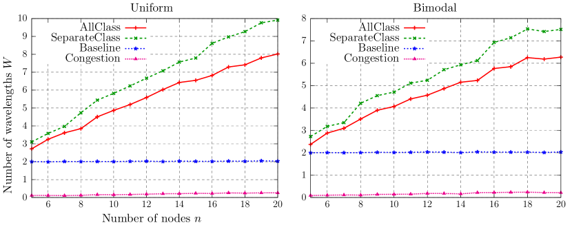
(a) Low Load

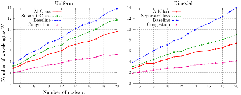
(b) High Load

Figure 4: Simulation results

For low load, the baseline algorithm outperforms our algorithms. At this level of traffic, it does not make sense to reserve different light-trails for different classes. However, as load increases our algorithms outperform the baseline algorithm.

For the same load, it is also seen that our algorithms become more effective as we change from the completely global Uniform distribution to the more local Bimodal distribution. This trend was also seen with the other distributions we experimented with.

Though we showed analytically that AllClass is not better than SeparateClass always, our simulation shows that AllClass performs better on the type of loads we generated. It may be noted that our algorithm for the stationary case mixes up the light-trails of different classes, and so suggests that the AllClass might work better in many practical scenarios.

8 Conclusions and Future Work

It can be shown that the non-splittable stationary problem is NP-hard, using a simple reduction from bin-packing. We do not know if the splittable problem is also NP-hard. We gave an algorithm for both variations of the stationary problem which takes $O(c+\log n)$ wavelengths. It will also be useful to improve the lower bound arguments; as Section 4 shows, congestion is not always a good lower bound. This may lead to a constant factor approximation algorithm for the problem.

In the on-line case we proved that the lower bound on the competitive ratio of any algorithm is $\Omega(\log n)$ and gave a matching algorithm which we proved to have competitive ratio $\Theta(\log n)$. We also gave a second algorithm which seems to work better in practice but can be as bad as $\Omega(\log^{2}n/\log\log n)$ factor worse than an optimal off-line algorithm on some pathological examples as we have shown. We also proved an upper bound of $O(\log^{2}n)$ for the algorithm but it will be an interesting problem to close the gap between the two bounds.

Our on-line model is very conservative in the sense that once a transmission is allocated on a light-trail, the light-trail cannot be modified. However, other models allow light-trails to shrink/grow dynamically [10]. It will be useful to incorporate this (with some suitable penalty, perhaps) into our model.

It will also be interesting to devise special algorithms that work well given the distribution of arrivals.

References

- [1] I. Chlamtac and A. Gumaste. Light-trails: A solution to IP centric communication in the optical domain. Lecture notes in computer science, pages 634–644, 2003.
- [2] A. Borodin and R. El-Yaniv. Online computation and competitive analysis. Cambridge University Press, New York, NY, USA, 1998.
- [3] D.D. Sleator and R.E. Tarjan. Amortized efficiency of list update and paging rules. Communications of the ACM, 28(2):202–208, 1985.
- [4] A.R. Karlin, M.S. Manasse, L. Rudolph, and D.D. Sleator. Competitive snoopy caching. Algorithmica, 3(1):79–119, 1988.
- [5] A. Gumaste and I. Chlamtac. Mesh implementation of light-trails: a solution to IP centric communication. Proceedings of the 12th International Conference on Computer Communications and Networks, ICCCN’03, pages 178–183, 2003.
- [6] A. Gumaste, G. Kuper, and I. Chlamtac. Optimizing light-trail assignment to WDM networks for dynamic IP centric traffic. In The 13th IEEE Workshop on Local and Metropolitan Area Networks, LANMAN’04, pages 113–118, 2004.
- [7] Y. Ye, H. Woesner, R. Grasso, T. Chen, and I. Chlamtac. Traffic grooming in light trail networks. In IEEE Global Telecommunications Conference, GLOBECOM’05, 2005.
- [8] A. Gumaste, J. Wang, A. Karandikar, and N. Ghani. MultiHop Light-Trails (MLT) - A Solution to Extended Metro Networks. Personal Communication.
- [9] S. Balasubramanian, W. He, and AK Somani. Light-Trail Networks: Design and Survivability. The 30th IEEE Conference on Local Computer Networks, pages 174–181, 2005.
- [10] A. Gumaste and I. Chlamtac. Light-trails: an optical solution for IP transport [Invited]. Journal of Optical Networking, 3(5):261–281, 2004.
- [11] Jing Fang, Wensheng He, and A.K. Somani. Optimal light trail design in WDM optical networks. In IEEE International Conference on Communications, volume 3, pages 1699–1703, June 2004.
- [12] A. Gumaste and P. Palacharla. Heuristic and optimal techniques for light-trail assignment in optical ring WDM networks. Computer Communications, 30(5):990–998, 2007.
- [13] A.S. Ayad, K.M.F. Elsayed, and S.H. Ahmed. Enhanced Optimal and Heuristic Solutions of the Routing Problem in Light Trail Networks. Workshop on High Performance Switching and Routing, HPSR’07, pages 1–6, 2007.
- [14] B. Wu and K.L. Yeung. OPN03-5: Light-Trail Assignment in WDM Optical Networks. In IEEE Global Telecommunications Conference, GLOBECOM’06, pages 1–5, 2006.
- [15] S. Balasubramanian, A.E. Kamal, and A.K. Somani. Network design in IP-centric light-trail networks. In 2nd International Conference on Broadband Networks, IEEE Broadnets’05, pages 41–50, 2005.
- [16] A. Lodha, A. Gumaste, P. Bafna, and N. Ghani. Stochastic Optimization of Light-trail WDM Ring Networks using Bender’s Decomposition. In Workshop on High Performance Switching and Routing, HPSR’07, pages 1–7, 2007.
- [17] W. Zhang, G. Xue, J. Tang, and K. Thulasiraman. Dynamic light trail routing and protection issues in WDM optical networks. In IEEE Global Telecommunications Conference, GLOBECOM’05, pages 1963–1967, 2005.
- [18] A. Gumaste and S.Q. Zheng. Dual auction (and recourse) opportunistic protocol for light-trail network design. In IFIP International Conference on Wireless and Optical Communications Networks, page 6, 2006.
- [19] Rajeev Wankar and Rajendra Akerkar. Reconfigurable architectures and algorithms: A research survey. IJCSA, 6(1):108–123, 2009.
- [20] K. Bondalapati and V.K. Prasanna. Reconfigurable meshes: Theory and practice. In Fourth Workshop on Reconfigurable Architectures, IPPS, 1997.
- [21] K. Nakano. A bibliography of published papers on dynamically reconfigurable architectures. Parallel Processing Letters, 5(1):111–124, 1995.
- [22] Y. Ben-Asher, D. Peleg, R. Ramaswami, and A. Schuster. The power of reconfiguration. Journal of parallel and distributed computing, 13(2):139–153, 1991.
- [23] J. Rothstein. Bus automata, brains, and mental models. IEEE Transactions on Systems, Man, and Cybernetics, 18(4):522–531, 1988.
- [24] L. Snyder. Introduction to the Configurable, Highly Parallel Computer. Computer, 15(1):47–64, 1982.
- [25] C.C. Weems, S.P. Levitan, A.R. Hanson, E.M. Riseman, D.B. Shu, and J.G. Nash. The image understanding architecture. International Journal of Computer Vision, 2(3):251–282, 1989.
- [26] E. Hao, PD MacKenzie, and QF Stout. Selection on the reconfigurable mesh. In Fourth Symposium on the Frontiers of Massively Parallel Computation, pages 38–45. IEEE, 1992.
- [27] R. Lin and S. Olariu. Reconfigurable Buses with Shift Switching: Concepts and Applications. IEEE Transactions on Parallel and Distributed Systems, 6(1):93–102, 1995.
- [28] J.L. Trahan, R. Vaidyanathan, and R.K. Thiruchelvan. On the Power of Segmenting and Fusing Buses. Journal of Parallel and Distributed Computing, 34(1):82–94, 1996.
- [29] S. Sahni. Data manipulation on the distributed memory bus computer. Parallel processing letters, 5(1):3–14, 1995.
- [30] S. Rajasekaran. Mesh Connected Computers with Fixed and Reconfigurable Buses: Packet Routing, Sorting, and Selection. In Proceedings of the First Annual European Symposium on Algorithms, pages 309–320. Springer-Verlag, 1993.
- [31] M. Maresca. Polymorphic Processor Arrays. IEEE Transactions on Parallel and Distributed Systems, 4(5):490–506, 1993.
- [32] H. Li and M. Maresca. Polymorphic-Torus Network. IEEE Transactions on Computers, 38(9):1345–1351, 1989.
- [33] J.W. Jang and V.K. Prasanna. An optimal sorting algorithm on reconfigurable mesh. Journal of Parallel and Distributed Computing, 25(1):31–41, 1995.
- [34] M. Geréb-Graus and T. Tsantilas. Efficient optical communication in parallel computers. In Proceedings of the fourth annual ACM symposium on Parallel algorithms and architectures, pages 41–48. ACM, 1992.
- [35] S. Pavel and S.G. Akl. Matrix operations using arrays with reconfigurable optical buses. International Journal of Parallel, Emergent and Distributed Systems, 8(3):223–242, 1996.
- [36] Yi Pan and Keqin Li. Linear array with a reconfigurable pipelined bus system—concepts and applications. Inf. Sci., 106(3-4):237–258, 1998.
- [37] R. Miller, VK Prasanna-Kumar, D.I. Reisis, and Q.F. Stout. Parallel Computations on Reconfigurable Meshes. IEEE Transactions on Computers, 42(6):678–692, 1993.
- [38] K. Li, Y. Pan, and S.Q. Zheng. Parallel matrix computations using a reconfigurable pipelined optical bus. Journal of Parallel and Distributed Computing, 59(1):13–30, 1999.
- [39] K. Nakano. Prefix-sums algorithms on reconfigurable meshes. Parallel processing letters, 5(1):23–35, 1995.
- [40] CP Subbaraman, J.L. Trahan, and R. Vaidyanathan. List ranking and graph algorithms on the reconfigurable multiple bus machine. In Parallel Processing, 1993. ICPP 1993. International Conference on, volume 3, 1993.
- [41] Y.R. Wang. An efficient O (1) time 3D all nearest neighbor algorithm from image processing perspective. Journal of Parallel and Distributed Computing, 67(10):1082–1091, 2007.
- [42] Y. Pan, M. Hamdi, and K. Li. Efficient and scalable quicksort on a linear array with a reconfigurable pipelined bus system. Future Generation Computer Systems, 13(6):501–513, 1998.
- [43] B.F. Wang and G.H. Chen. Two-dimensional processor array with a reconfigurable bus system is at least as powerful as CRCW model. Information Processing Letters, 36(1):31–36, 1990.
- [44] K. Li, Y. Pan, and S.Q. Zheng. Efficient deterministic and probabilistic simulations of PRAMs on linear arrays with reconfigurable pipelined bus systems. The Journal of Supercomputing, 15(2):163–181, 2000.
- [45] Torsten Suel. Routing and sorting on meshes with row and column buses. In Proceedings of the Eighth International Symposium on Parallel Processing, pages 411–417. IEEE, 1994.
- [46] S. Rajasekaran and S. Sahni. Sorting, selection, and routing on the array with reconfigurable optical buses. IEEE Transactions on Parallel and Distributed Systems, 8(11):1123–1132, 1997.
- [47] E. G. Coffman, Jr., M. R. Garey, and D. S. Johnson. Approximation algorithms for bin packing: a survey. Approximation algorithms for NP-hard problems, pages 46–93, 1997.
- [48] S. Olariu. An optimal greedy heuristic to color interval graphs. Information Processing Letters, 37(1):21–25, 1991.