Magnetospheric Accretion and Ejection of Matter in Resistive Magnetohydrodynamic Simulations

Abstract

The ejection of matter in the close vicinity of a young stellar object is investigated, treating the accretion disk as a gravitationally bound reservoir of matter. By solving the resistive MHD equations in 2D axisymmetry using our version of the Zeus-3D code with newly implemented resistivity, we study the effect of magnetic diffusivity in the magnetospheric accretion-ejection mechanism. Physical resistivity was included in the whole computational domain so that reconnection is enabled by the physical as well as the numerical resistivity. We show, for the first time, that quasi-stationary fast ejecta of matter, which we call micro-ejections, of small mass and angular momentum fluxes, can be launched from a purely resistive magnetosphere. They are produced by a combination of pressure gradient and magnetic forces, in presence of ongoing magnetic reconnection along the boundary layer between the star and the disk, where a current sheet is formed. Mass flux of micro-ejection increases with increasing magnetic field strength and stellar rotation rate, and is not dependent on the disk to corona density ratio and amount of resistivity.

1. Introduction

Highly collimated outflows have been observed from AGNs to Young Stellar Objects (YSOs) and young brown dwarfs (Whelan et al., 2005, 2007). Accreting compact stars, like accreting white dwarfs in symbiotic binaries (Sokoloski & Kenyon, 2003) and neutron stars like Cir X-1 (Heinz et al., 2007), also show similar outflowing phenomena. An outflow is characterized as a jet if it is super-magnetosonic, collimated into an apparent narrow opening, and reaches a stationary or quasi-stationary state. Such high-velocity outflowing fluxes of matter are an integral part of stellar evolution. Observations in multiple wavelengths are reaching closer and closer to the objects that drive them.

Among all the systems, models of launching outflows in YSOs are closest to scrutiny by observations due to available data from star–forming regions. An accretion disk, through which matter accretes onto the young star with velocities close to a free–fall, is often associated with a jet–driving YSO (Edwards et al., 1994, 2006). A correlation between the accretion rate and the high-velocity jet power was found in many Classical T-Tauri Stars (CTTSs) (Cabrit et al., 1990). The ratio of mass loss in the outflow to disk accretion rate, $\dot{M}_{\rm w}/\dot{M}_{\rm a}$, extracted from observations is hard to constrain. It is best estimated to be approximately 0.1 through measurements of optical forbidden lines and veiling — see e.g. Hartigan et al. (1995) and Edwards (2008). Recently, He I $\lambda$10830 line has been used as a probe into the high-velocity winds originating from the inner region where the star interacts with the disk (Edwards et al., 2003; Kwan et al., 2007). Despite the potential diagnostic power of such emission lines, the actual structure and physical conditions of outflows can be more complex. Star-disk interaction is also investigated by means of X-rays, which offer deepest probe into the launching region. During flare events from the protostellar objects X-rays are emitted and have been observed (Favata et al. (2005), Giardino et al. (2006), Aarnio et al. (2010), McCleary & Wolk (2011)). Production of such X-rays is possible by either high temperature or high flow velocities, which can be related to the stellar surface, shocks in the stellar magnetosphere or, as we will suggest, to the reconnection events in the star-disk magnetosphere. Such events will leave imprint in the chemical and physical properties of the object (Shu et al., 2007). To further interpret the observed line profiles, and the origins of outflows from the close vicinity of CTTSs, predictions from both theoretical and numerical models are required.

Table 1In many resistive-MHD simulations performed up to date, assumptions for initial conditions vary much and duration of simulations is very different. We list some of important works to position our work in the context. In the second column, “fast” stellar rotation means that corotation radius is smaller than the disk truncation radius, $R_{cor}<R_{t}$ and “slow” rotation means that $R_{cor}>R_{t}$. Disk is rotating in all the cases. Columns about physical resistivity and viscosity specify only if the option is at all included in the code; for where it is really effective, reader should check the related publication. When present, viscosity is important only in the disk.

	$\Omega_{\ast}$	corona	$\kappa=\rho_{d}/\rho_{c}$	$T_{\mathrm{m}ax}/T_{0}$ (days)	resistive	viscous
Hayashi et al. (1996)	non-rotating	non-rotating	103	5	yes	no
Hirose et al. (1997)	non-rotating	rotating	104	16.5	yes	no
		rotating different than disk
Miller & Stone (1997)	slow	solid body rotation	102	0.3	yes	no
		corotating with star at $R_{\rm cor}$
Goodson et al. (1999)	fast	rotating	$10^{4}$	100	yes	no
Romanova et al. (2002)	slow	corotating with star	102	100	no	yes
		for R$\leq R_{\rm cor}$, else with disk
Küker et al. (2003)	slow	not in hydrostatic balance,	103	1000	yes	yes
		non-rotating
Ustyugova et al. (2006)	fast	corotating with star	103	2000	yes	yes
		for R$\leq R_{\rm cor}$, else with disk
Romanova et al. (2009)	fast	corotating with star	104	2000	yes	yes
	and slow	for R$\leq R_{\rm cor}$, else with disk
MČ et al. (present paper)	slow	corotating with star	104	1500	yes	no
		for R$\leq R_{\rm cor}$, else with disk

Outflows driven by energy derived from accretion are particularly appealing in the scenarios of jet launching. Many models have been proposed based on the concept of magnetocentrifugal wind mechanisms (Blandford & Payne, 1982), differing in the origins of the underlying magnetic fields and locations of matter launching. An outflow could be a disk wind driven by magnetic fields dragged in from the envelope or generated by the disk dynamo, or an inner disk wind anchored to the narrow innermost region as in the X-wind model powered by an enhanced dynamo from the star-disk interaction (Shu et al., 1994, 1997), simultaneously with an accretion funnel (Ostriker & Shu, 1995). It might also be a stellar wind driven along the open field lines from the stellar surface by thermal or magnetic pressure (Matt & Pudritz, 2005, 2008), or some combination of the different possibilities. Related to the launch of winds, magnetospheric accretion has been described in works by Königl (1991), Ostriker & Shu (1995) and Koldoba et al. (2002) in the context of a magnetosphere interacting with the surrounding disk, sharing some similarities with the compact objects like neutron stars (Ghosh & Lamb, 1979a, b). Except for the pure disk wind models, a magnetically connected star-disk system plays an important role in the making of the young stellar system and the evolution of angular momentum through the generation of outflows during the main phase of accretion.

Numerical investigations have been followed up on the time-dependent evolution of a system where the central star is magnetically connected to its accretion disk and their connection to jet formation and accretion. In one of the earliest attempts by Hayashi et al. (1996), where simulations of only a few rotation periods were obtained, a dipole magnetosphere corotating with the central star threaded the accretion disk that was in Keplerian rotation. Magnetic field lines connecting both the disk and the star inflate outwards due to shear, and reconnection blows out the matter along with the field, partially opening up the originally closed dipole loops. Gas can outflow from those opened field lines and might form part of the X-emission that is often associated with flares. Reconnection as a possible origin of X-rays from such systems has also been indicated in dal Pino et al. (2010). Hirose et al. (1997) investigated a magnetized star interacting with a truncated disk that was threaded with an initially uniform field dragged in from the outer core, in the same direction of the magnetosphere, but separated by a neutral current sheet in the equatorial plane as a result of interaction between the fields brought together. For simplicity, the star was not rotating, but the differentially rotating disk could anyway provide enough shear to make the field inflate outwards, followed by a reconnection event and mass transfer onto the magnetosphere. The transferred mass diverted into two directions: one that falls onto the star and the other that flows out along the opened stellar field lines.

Longer simulations by Goodson et al. (1997) with an aligned dipole and a conducting accretion disk showed that differential rotation of the disk can drive episodes of loop expansion. Such expansion can drive two outflow components of gas: one hot convergent flow along the rotation axis, and another, slower cold flow on the disk side of the expanding loop. Miller & Stone (1997), on the other hand, investigated interactions of magnetospheres with accretion disks under three different magnetic configurations and their respective dynamical evolution.

Küker et al. (2003) solved the disk in 1D with a radiative hydrodynamic code by Kley (1989), and then extrapolated the solution to 2D as their initial condition. For the full 2D axisymmetric MHD problem, the induction equation, Lorentz force and Ohmic dissipation were now included into Kley’s code, with the assumption of equal viscous and resistive dissipations. With $Pr\sim 1$ magnetic field lines would not bend towards the axis. However, because of non-equilibrium initial conditions, they bunched close to the star. The main result was that, with the assumed mass accretion rate of $\dot{M}_{0}=10^{-7}M_{\odot}$ yr^-1, for a smaller magnetic field than 1 kG the disk was not disrupted; but for a larger field of the order of 1-10 kG, an outflow could be launched from the disk. In Romanova et al. (2002) and Long et al. (2005), much better initial equilibrium has been set than in any previous simulations, with matter continuing to inflow through the disk because of viscosity. It was an improvement, as it was proceeding with the viscous time-scale, because of a slow accretion of matter. Without such initial equilibrium, the non-stationary initial conditions determine the flow in the disk, and influence the simulation. A star and part of the magnetosphere corotated up to the corotation radius, and the magnetosphere corotated with the disk farther out. The simulations were performed in the ideal MHD regime, with effective numerical resistivity diffusing magnetic field in the radial direction. They found funnel flows onto the central object, spinning up or down the star, depending on the ratio of rotation rate of the star to the rotation rate of the disk inner rim.

In Ustyugova et al. (2006) and Romanova et al. (2009) the effects of physical viscosity and resistivity on the outflow were investigated. In Romanova et al. (2009) one of studied cases is with the magnetic Prandtl number, the ratio between the viscosity and the resistivity $\mathrm{Pr}=\nu/\eta$, greater than one. Magnetic field lines are bent towards the magnetosphere in the gap and magnetic energy increases, enabling the outflow. It has been found that, in addition to the fast and light jet, there is another, new conical wind flowing up to 30 percent of the matter from the innermost portion of the disk. Two different cases were considered in their simulations, one for a fast (with the setup as in Ustyugova et al. (2006) and a slightly different parameters), and the other for a slowly rotating star. In both cases, to enable the smooth start of the simulation, initially slow rotation of the star was gradually speeded up to its maximum value, with matter slowly inflowing from the outer boundary, to obtain stellar magnetic field compressed towards the magnetosphere in the gap. In the latter case, disk was not initially present in the computational box, but was formed from the matter inflowing from the outer boundary. Such setup was different from most other simulations in the literature.

With non-stationary initial conditions in the disk, accretion tends to be too fast. Most of the mentioned works involve resistive MHD models of accretion disks. Introduction of viscosity in the disk helps to obtain slow accretion, with a viscous time-scale. We do not include physical viscosity in our simulations, but we set the resistivity in the whole computational box, not only in the disk. Resistivity, which controls the onset of magnetic reconnection, triggers the necessary change in the magnetic field geometry needed for any launching. In our previous work, in Čemeljić & Fendt (2004), we reported on the result (with the same code) when only a disk is present, without the magnetosphere of the central object taken into account. Propagation of the outflow through the resistive corona (with the disk set as a boundary condition) we investigated in Fendt & Čemeljić (2002).

One important parameter to distinguish the investigated MHD regime is the already mentioned magnetic Prandtl number. As there is no physical viscosity included, our resistive simulations are in the regime of $\mathrm{Pr}\lesssim 1$. Violent initial conditions now helped to bring magnetic flux closer towards the star, helping the launching of matter outwards. Another parameter whose effect we study is the density ratio between the disk and the corona. It is usually included as a free parameter of the order of $10^{2}$ or $10^{3}$, at best $10^{5}$. We investigate the influence of this ratio on the mass and angular momentum flux in the launching of outflows. There are other possibilities in the setup, which we did not investigate here, e.g. inclusion of the stellar wind, which would probably affect the open stellar field.

Table 1 lists the kinematic and thermodynamic assumptions adopted in earlier works, each of them being usually repeated with a variety of parameters or methods, with or without physical resistivity and viscosity included in the code. We put our work in context of setups and assumptions of those works, as our results differ in the mass fluxes carried in the ejected gas.

The organization of the paper is as follows. We first describe our implementation of the boundary and initial conditions. In §4 we report regimes we found under a broad range of parameters. We investigated the influence of corona to disk density ratio, strength of magnetic field and the physical resistivity. In §5 we address the role of reconnection in the launching, in §6 we check a criterion for the site of launching, and in §7 we compare position of the disk truncation radius in our simulations with some theoretical predictions. Then we discuss investigated parameters and the resulting ejections.

2. Numerical Setup for the Resistive MHD System

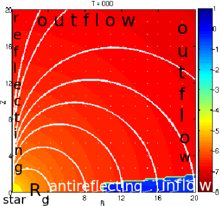
Figure 1.— Initial and boundary conditions in our simulations. The initial hydrostatic density distribution in the disk corona and the disk is plotted in logarithmic color grading. The density in the disk is four orders of magnitude larger than in the corona. The dipole stellar magnetic field is plotted in white solid lines, and velocity vectors are shown in white arrows. The stellar surface is defined as a rotating absorbing boundary layer, enclosing the origin — see the zoom into this region in Figure 2. In simulation S2, the stellar absorbing layer extends into the small portion of the disk mid-plane inside the disk gap, of radius $R_{g}$, as an outflow boundary. Along the axis of symmetry and at the mid-plane in the disk, a reflection and anti-reflection boundaries are imposed. An outflow boundary is imposed on the outer boundaries of the computational domain, except for the disk outer rim, where a small inflow into the disk is set, to mimic the accretion flow from the portion of the disk beyond the computational box.

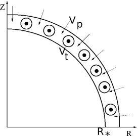
Figure 2.— Zoom into the setup of the stellar surface from the Figure 1. The star is set as a rotating, absorbing boundary condition inside the computational box, enclosing the origin. Components of the poloidal velocity $v_{\mathrm{p}}$ are copied from the layer immediately above the star. The stellar rotation rate, determined by the initial toroidal component of the velocity $v_{\mathrm{t}}$ at the stellar surface, is kept constant throughout the simulation.

We extend previous work of Čemeljić & Fendt (2004), who adopted a disk in the resistive MHD regime and its halo in the ideal-MHD regime, following Casse & Keppens (2002). We implement an absorbing, rotating stellar surface layer enclosing the origin, and include resistivity in the whole computational box. It is an anomalous, turbulent resistivity parametrized by Alfvénic velocity as a characteristic velocity, resulting in $\eta\sim\rho^{1/3}$, as derived in Fendt & Čemeljić (2002). We limited its value to few orders of magnitude above the numerical resistivity, but leaving it large enough to facilitate reconnection everywhere in the computational box. Our resistivity is not limited only to the region nearby the disk, as we simulate innermost part of the star-disk system, nearby the gap, enclosing only $0.2\times 0.2$ AU. Hence we anticipate presence of the turbulence, and with it, resistivity, in the whole computational box. The initial conditions of density and magnetic field are shown in Figure 1, and the setup of the stellar surface as a boundary layer inside the computational box is shown in Figure 2.

The equations of resistive MHD are solved using our version of the Zeus-3D code, Zeus347 (Fendt & Čemeljić, 2002), in axisymmetry option. They are, in the cgs system of units:

$${\frac{\partial\rho}{\partial t}}+\nabla\cdot(\rho\mathchoice{\mbox{\boldmath$\displaystyle\rm v$}}{\mbox{\boldmath$\textstyle\rm v$}}{\mbox{\boldmath$\scriptstyle\rm v$}}{\mbox{\boldmath$\scriptscriptstyle\rm v$}})=0$$ (1)

$$\rho\left[{\frac{\partial\mathchoice{\mbox{\boldmath$\displaystyle\rm v$}}{\mbox{\boldmath$\textstyle\rm v$}}{\mbox{\boldmath$\scriptstyle\rm v$}}{\mbox{\boldmath$\scriptscriptstyle\rm v$}}}{\partial t}}+\left(\mathchoice{\mbox{\boldmath$\displaystyle\rm v$}}{\mbox{\boldmath$\textstyle\rm v$}}{\mbox{\boldmath$\scriptstyle\rm v$}}{\mbox{\boldmath$\scriptscriptstyle\rm v$}}\cdot\nabla\right)\mathchoice{\mbox{\boldmath$\displaystyle\rm v$}}{\mbox{\boldmath$\textstyle\rm v$}}{\mbox{\boldmath$\scriptstyle\rm v$}}{\mbox{\boldmath$\scriptscriptstyle\rm v$}}\right]+\nabla p+\rho\nabla\Phi-\frac{\mathchoice{\mbox{\boldmath$\displaystyle j$}}{\mbox{\boldmath$\textstyle j$}}{\mbox{\boldmath$\scriptstyle j$}}{\mbox{\boldmath$\scriptscriptstyle j$}}\times\mathchoice{\mbox{\boldmath$\displaystyle B$}}{\mbox{\boldmath$\textstyle B$}}{\mbox{\boldmath$\scriptstyle B$}}{\mbox{\boldmath$\scriptscriptstyle B$}}}{c}=0$$ (2)

$${\frac{\partial\mathchoice{\mbox{\boldmath$\displaystyle B$}}{\mbox{\boldmath$\textstyle B$}}{\mbox{\boldmath$\scriptstyle B$}}{\mbox{\boldmath$\scriptscriptstyle B$}}}{\partial t}}-\nabla\times\left(\mathchoice{\mbox{\boldmath$\displaystyle\rm v$}}{\mbox{\boldmath$\textstyle\rm v$}}{\mbox{\boldmath$\scriptstyle\rm v$}}{\mbox{\boldmath$\scriptscriptstyle\rm v$}}\times\mathchoice{\mbox{\boldmath$\displaystyle B$}}{\mbox{\boldmath$\textstyle B$}}{\mbox{\boldmath$\scriptstyle B$}}{\mbox{\boldmath$\scriptscriptstyle B$}}-{\frac{4\pi}{c}}\eta\mathchoice{\mbox{\boldmath$\displaystyle j$}}{\mbox{\boldmath$\textstyle j$}}{\mbox{\boldmath$\scriptstyle j$}}{\mbox{\boldmath$\scriptscriptstyle j$}}\right)=0$$ (3)

$$\rho\left[{\frac{\partial e}{\partial t}}+\left(\mathchoice{\mbox{\boldmath$\displaystyle\rm v$}}{\mbox{\boldmath$\textstyle\rm v$}}{\mbox{\boldmath$\scriptstyle\rm v$}}{\mbox{\boldmath$\scriptscriptstyle\rm v$}}\cdot\nabla\right)e\right]+p(\nabla\cdot\mathchoice{\mbox{\boldmath$\displaystyle\rm v$}}{\mbox{\boldmath$\textstyle\rm v$}}{\mbox{\boldmath$\scriptstyle\rm v$}}{\mbox{\boldmath$\scriptscriptstyle\rm v$}})=0$$ (4)

$$\mathchoice{\mbox{\boldmath$\displaystyle j$}}{\mbox{\boldmath$\textstyle j$}}{\mbox{\boldmath$\scriptstyle j$}}{\mbox{\boldmath$\scriptscriptstyle j$}}=\frac{c}{4\pi}\nabla\times\mathchoice{\mbox{\boldmath$\displaystyle B$}}{\mbox{\boldmath$\textstyle B$}}{\mbox{\boldmath$\scriptstyle B$}}{\mbox{\boldmath$\scriptscriptstyle B$}}\ ,$$ (5)

where we neglected the Ohmic term in the energy equation. For a complete set of equations, an ideal gas law is assumed. The symbols in the equations of continuity of mass, momentum and induction equation have their usual meaning: $\rho$ and $p$ are the matter density and thermal pressure, $\textstyle v$ is the velocity, $\Phi=-GM_{\ast}/(R^{2}+Z^{2})^{1/2}$ is the gravitational potential of the central object, and $\textstyle B$ and $\textstyle j$ are the magnetic field and the electrical current, respectively. In cgs units, magnetic diffusivity is equal to resistivity, so $\eta$ stands for the electrical resistivity. The resistive term in the induction equation (Equation 3) is included in the code by subtracting $4\pi\eta\mathchoice{\mbox{\boldmath$\displaystyle j$}}{\mbox{\boldmath$\textstyle j$}}{\mbox{\boldmath$\scriptstyle j$}}{\mbox{\boldmath$\scriptscriptstyle j$}}/c$ from the electromotive forces in the mocemfs procedure in Zeus347 — see Appendix A in Fendt & Čemeljić (2002) for tests. In the energy equation, $e=p/(\gamma-1)$ is the internal energy per unit volume, with an adiabatic index $\gamma=5/3$ in the initial conditions.

We solve these MHD equations in dimensionless form. The variables are normalized to their value measured in the mid-plane of the disk, at a fiducial radius $R_{0}$, which we choose to be inside the initial disk gap, $R_{0}=2.86R_{\ast}$, where $R_{\ast}$ is the stellar radius. We include radial distances up to 20 stellar radii in our computational box. Choice of the mass accretion rate for the disk fixes the fiducial density, from $\dot{M}_{0}=R_{0}^{2}\rho_{0}{\rm v}_{\rm K,0}$, and from the Keplerian velocity at $R_{0}$, which is ${\rm v}_{\rm K,0}=(GM_{\ast}/R_{0})^{1/2}$, we normalize the stellar mass and velocity unit in the code with $(GM_{\ast})^{1/2}=1$. The normalized coordinates are $R^{\prime}=R/R_{0}$, $Z^{\prime}=Z/R_{0}$, and $\mathchoice{\mbox{\boldmath$\displaystyle\rm v^{\prime}$}}{\mbox{\boldmath$\textstyle\rm v^{\prime}$}}{\mbox{\boldmath$\scriptstyle\rm v^{\prime}$}}{\mbox{\boldmath$\scriptscriptstyle\rm v^{\prime}$}}=\mathchoice{\mbox{\boldmath$\displaystyle\rm v$}}{\mbox{\boldmath$\textstyle\rm v$}}{\mbox{\boldmath$\scriptstyle\rm v$}}{\mbox{\boldmath$\scriptscriptstyle\rm v$}}/{\rm v}_{\rm K,0}$. The time in the code is measured in units of the rotation rate timescale at $R_{0}$, $t_{0}=R_{0}/{\rm v}_{\rm K,0}$, and the period at $R_{0}$ is equal to $2\pi$. The dimensionless equation of motion can be written as:

$$\frac{\partial\mathchoice{\mbox{\boldmath$\displaystyle\rm v$}}{\mbox{\boldmath$\textstyle\rm v$}}{\mbox{\boldmath$\scriptstyle\rm v$}}{\mbox{\boldmath$\scriptscriptstyle\rm v$}}^{\prime}}{\partial t^{\prime}}+\left(\mathchoice{\mbox{\boldmath$\displaystyle\rm v$}}{\mbox{\boldmath$\textstyle\rm v$}}{\mbox{\boldmath$\scriptstyle\rm v$}}{\mbox{\boldmath$\scriptscriptstyle\rm v$}}^{\prime}\cdot\nabla^{\prime}\right)\mathchoice{\mbox{\boldmath$\displaystyle\rm v$}}{\mbox{\boldmath$\textstyle\rm v$}}{\mbox{\boldmath$\scriptstyle\rm v$}}{\mbox{\boldmath$\scriptscriptstyle\rm v$}}^{\prime}=\frac{\mathchoice{\mbox{\boldmath$\displaystyle j$}}{\mbox{\boldmath$\textstyle j$}}{\mbox{\boldmath$\scriptstyle j$}}{\mbox{\boldmath$\scriptscriptstyle j$}}^{\prime}\times\mathchoice{\mbox{\boldmath$\displaystyle B$}}{\mbox{\boldmath$\textstyle B$}}{\mbox{\boldmath$\scriptstyle B$}}{\mbox{\boldmath$\scriptscriptstyle B$}}^{\prime}}{M_{\rm A,0}^{2}\,\rho^{\prime}}-\frac{\nabla^{\prime}p^{\prime}}{\delta_{0}\,\rho^{\prime}}-\nabla^{\prime}\Phi^{\prime}\,,$$ (6)

with $\nabla^{\prime}=R_{0}\nabla$, $t^{\prime}=t/t_{0}$, $\rho^{\prime}=\rho/\rho_{0}$, $\mathchoice{\mbox{\boldmath$\displaystyle B$}}{\mbox{\boldmath$\textstyle B$}}{\mbox{\boldmath$\scriptstyle B$}}{\mbox{\boldmath$\scriptscriptstyle B$}}^{\prime}=\mathchoice{\mbox{\boldmath$\displaystyle B$}}{\mbox{\boldmath$\textstyle B$}}{\mbox{\boldmath$\scriptstyle B$}}{\mbox{\boldmath$\scriptscriptstyle B$}}/\mathchoice{\mbox{\boldmath$\displaystyle B$}}{\mbox{\boldmath$\textstyle B$}}{\mbox{\boldmath$\scriptstyle B$}}{\mbox{\boldmath$\scriptscriptstyle B$}}_{\rm 0}$ and $\Phi^{\prime}=-1/(R^{\prime 2}+Z^{\prime 2})^{1/2}$. Primes are omitted in equations in the rest of this paper, and quantities are written in code units, unless otherwise specified.

We introduced the free parameters:

$$M_{\rm A,0}^{2}\equiv 4\pi\rho_{\rm 0}{\rm v}^{2}_{\rm K,0}/B_{\rm 0}^{2}\ {\rm and}\ \delta_{\rm 0}\equiv\rho_{\rm 0}{\rm v}^{2}_{\rm K,0}/p_{\rm 0}\ .$$ (7)

The Alfvénic Mach number, $M_{\rm A,0}$, at $R_{0}$ and $Z=0$, determines the magnetic field strength. In a typical run, $M_{\rm A,0}=225$ for a dipole field of the order of 100 G, at the surface of the star. The kinetic to thermal energy density ratio, $\delta_{\rm 0}$, is the square of the gas Mach number, whose fiducial value can be estimated from the definition of the adiabatic coefficient. For our setup we choose $\delta_{\rm 0}=100$ or 50. The typical temperatures in the corona and the disk of the YSOs are $10^{6}\,K$ and $5\times 10^{3}\,K$, respectively, so that at the inner edge of the disk initially should be $c_{\mathrm{s},corona}/c_{\mathrm{s},disk}=20$. Our initial disk is initially for an order of magnitude too hot, so that this ratio is about 6 times smaller.

We use a uniform grid of $R\times Z=(90\times 90)$ cells, in the axisymmetric cylindrical coordinates $(R,\phi,Z)$. The physical scale corresponds to $(20\times 20)$ stellar radii. We note that our simulations do not scale well: it was not easy to obtain results in other resolutions or domains. We performed larger domain simulations in $R\times Z=(40\times 40)R_{\ast}$ with the same resolution, and simulations in higher resolution with $R\times Z=(180\times 180)$ grid cells in $(20\times 20)R_{\ast}$. Such simulations lasted long enough for verification, but are more prone to numerical problems, and tend to cease during the relaxation or soon afterwards, so that it is harder to perform a thorough parameter study using them. This is probably because of numerical viscosity $\nu_{\mathrm{n}um}=v\Delta x$, which is larger with less resolution $\Delta x$ ($v$ is the characteristic velocity), and helps the code to go through problematic events. Inclusion of physical viscosity would probably enable better resolution, but we focus here only on the effects of resistivity.

2.1. Example of rescaling

We give an example of rescaling for a case of an YSO with stellar mass of $M_{\ast}=0.8M_{\odot}$ and radius $R_{\ast}=2R_{\odot}$, so that fiducial distance is $R_{0}=2.86R_{\ast}=5.7R_{\odot}=0.027$ AU. Our computational domain is then $R\times Z\approx 0.2\times 0.2$ AU. We can rewrite the Keplerian speed at $R_{0}$ in units of solar mass and radius as

$${\rm v}_{\rm K,0}=\sqrt{\frac{GM_{\ast}}{R_{\rm 0}}}=\sqrt{\frac{GM_{\odot}}{R_{\odot}}}\sqrt{\frac{M_{\ast}}{M_{\odot}}\big{/}\left(\frac{R_{\rm 0}}{R_{\odot}}\right)}\ ,$$ (8)

giving the fiducial velocity $1.64\times 10^{7}$ cm s${}^{-1}=164~{}$km s^-1. The period of Keplerian rotation at $R_{0}$ is $P_{0}=2\pi R_{0}/{\rm v}_{\rm K,0}=1.76$ days. The stellar rotation rate for T-Tauri Stars is usually about $1/10$ of the breakup rate, which we obtain from $(GM_{\ast}/R_{\ast}^{3})^{1/2}=2\times 10^{-4}\mathrm{s}^{-1}=0.4$ days. This gives a typical period of rotation of a star about 4 days. If we assume an accretion rate of $\dot{M}_{0}=10^{-8}M_{\odot}$ yr^-1, fiducial density and pressure are $\rho_{0}=2.44\times 10^{-13}$ g cm^-3 and $p_{0}=109$ erg cm^-3, respectively. With $c_{\rm s}\sim{\rm v}_{\rm K,0}$, the reference temperature is $T_{0}=m{\rm v}_{\rm K,0}^{2}/(\gamma\Re)\sim 10^{6}$ K. Estimate of the initial temperature at R${}_{i}=10R_{\ast}$ in the disk gives $5.5\times 10^{4}$ K, and in the corona it is 5 times larger, $2.7\times 10^{6}$ K. The sound speed in the disk has been estimated as $\sim{\rm v}_{\rm K,0}$, and in the corona, in the part corotating with the star, as $\sim 0.1R_{i}\Omega_{\ast}$. The reference value of resistivity is $\eta_{0}\sim{\rm v}_{\rm K,0}R_{0}=10^{19}$cm${}^{2}s^{-1}$, which is much larger than the classical Spitzer value.

The strength of the magnetic field we obtain from the magnetic pressure at the mid-plane of the disk, $B_{0}(Z=0)=(4\pi p_{0}\delta_{0})^{1/2}/M_{\rm A,0}$ (see Equation 7), and the stellar dipole field at $R_{0}$ is $B_{0}=B_{\ast}(R_{\ast}/R_{0})^{3}$. A complete expression for the fiducial magnetic field we can write in units of solar mass and radius as:

$$B_{0}^{2}=\frac{4\pi}{M_{\rm A,0}^{2}}\frac{\dot{M}_{\rm a}}{M_{\odot}/{\mathrm{y}r}}\frac{M_{\odot}}{\mathrm{y}r}\sqrt{\frac{GM_{\odot}}{R_{\odot}^{5}}\frac{M_{\ast}/M_{\odot}}{(R_{0}/R_{\odot})^{5}}}\,.$$ (9)

The factor $4\pi$ is required to obtain the Gaussian cgs value from the implicit normalization of the magnetic field in the ZEUS code. When the surface strength of the dipole magnetic field is combined with Equation 9, it gives

$$B_{\ast}=\frac{667~{}{\rm Gauss}}{M_{\rm A,0}}\sqrt{\dot{M}_{8}}\,,$$ (10)

where $\dot{M}_{8}$ is the disk mass accretion rate in units of $10^{-8}M_{\odot}$ yr^-1. For $\dot{M}_{8}=100$ and $M_{A,0}=35$, $B_{\ast}$ is about 200 G.

2.2. Boundary conditions

Figure 3.— Initial angular velocity profiles along the disk mid-plane in our setups. Shown are the angular velocities in simulations with the stellar rotation rate $\Omega_{\ast}=$0.15, 0.1 and 0.068, in short-dashed, solid and long-dashed line, respectively. For comparison, the dotted line shows the Keplerian rotation profile. The kink in the initial rotational profile is near the initial inner disk radius $R_{\mathrm{i}}$.

In order to mimic an absorbing stellar surface, we define the “outflow” boundary condition around a central object. As done by Uchida & Shibata (1985), we define part of the computational box surrounding the origin as a boundary layer, for a region further above the star. We set up a rotating circular layer of one grid cell thickness on top of the star, at a distance $R_{\ast}$ from the origin, with the stellar rotation rate $\Omega_{\ast}$ as a free parameter – see Figure 2. All the other hydrodynamical quantities are absorbed, so that the values in this layer are copied from the cells immediately above it. With this procedure, we neglect the stellar wind.

The outer boundaries of our computational box are open, with the flows extrapolated beyond the boundary. One exception is a small part at the disk outer boundary. There, we prescribe a small mass inflow that is consistent with the initial radial component of the velocity in the disk. Reflection boundaries are imposed along the axis of symmetry and, in simulation S1, at the disk mid-plane inside the disk, where the normal component of the magnetic field is continuous, the tangential component is reflected, and the toroidal magnetic field is anti-reflected. Under axisymmetry for the disk mid-plane and the axis, $B_{R}(R=0,Z)=B_{R}(R,Z=0)=0$, and with these conditions $\nabla\cdot\mathchoice{\mbox{\boldmath$\displaystyle B$}}{\mbox{\boldmath$\textstyle B$}}{\mbox{\boldmath$\scriptstyle B$}}{\mbox{\boldmath$\scriptscriptstyle B$}}=0$ is satisfied. We use the Constrained Transport (CT) method of Evans & Hawley (1988) to ensure that it is preserved to a machine round-off precision in computations.

In simulation S2, we treat a small part of the disk mid-plane inside the disk gap as an “outflow” boundary, extrapolating the flow from the active zones into the ghost zones, effectively extending the stellar absorbing layer into the disk gap. All the values in the ghost zones are set equal to the values in the corresponding active zones, and the angular velocity and toroidal component of the magnetic field are projected. This ensures preservation of the disk gap in the simulation, even when the magnetic field is not strong enough to truncate the disk. This means that some other physical effects, which we do not include in our simulations, would have to act in terminating the disk. It could be that material which actually resides in the disk gap is not well described by our approximations, or that influence of additional forces, as the radiation pressure force from the central object, which we neglect here, is large. Using such a setup, we can study if a weaker stellar dipole can launch matter from the innermost magnetosphere. Caveat is that the final disk truncation radius in simulation S2 is then dependent on the boundary conditions, and is not self-consistently computed.

2.3. Initial conditions

We set up initial conditions for the density distribution, velocity profiles, magnetic field and resistivity in the computational domain as follows. Gravitationally bound disk rotates slightly sub-Keplerian. For a self-consistent accretion disk, additional constraints such as constant fluxes through surfaces at different radii and stability to various modes of oscillation should be included. However, the disk stability or the accretion process itself is not the subject of study here, and we treat the disk only as a supply of matter into the stellar magnetosphere.

2.3.1 Density distribution

The initial disk density distribution is

$$\rho_{\rm d}(R,Z)=\frac{R_{\rm off}^{3/2}}{(R_{\rm off}^{2}+R^{2})^{3/4}}\times$$

$$\left(\max\{10^{-6}\ ,\ \left[1-\frac{(\gamma-1)Z^{2}}{2H^{2}}\right]\}\right)^{1/(\gamma-1)}\,,$$ (11)

shown in Figure 1. The density is limited by the maximum function, and ensured to be regular by a constant offset radius $R_{\rm off}=4$. The disk is adiabatic with an index $\gamma=5/3$, and physically thin, with an aspect ratio of $H/R=0.1$, where $H$ is the disk height at a given radius $R$. For the initial inner disk radius we tried various initial positions of the initial inner disk radius $R_{\rm i}$ in our parameter study; here it is chosen to be at half size of the computational domain, $R_{\rm i}=10R_{\ast}$. It is not a critical parameter, as the disk will adjust its inner rim position during the simulation, but too close positioned $R_{\rm i}$ can, especially in a case of strong magnetic field, result in a too violent initial relaxation, which will stop a simulation.

The corona above the star and in the disk gap corotate with the central object, and further away, with the underlying disk. The corona is in hydrostatic balance, with an initial coronal density:

$$\rho_{\rm c}(R,Z)=\frac{(R^{2}+Z^{2})^{-3/4}}{\kappa}\,,$$ (12)

which is obtained from the equality of gravitational and hydrostatic pressure. Such a corona, when rotating, is not in an equilibrium, and the different rotation rates of the corona in the inner portion of the computational box and above the disk is making it even further from equilibrium. The free parameter $\kappa=\rho_{\rm d}/\rho_{\rm c}$ determines density in the corona. In similar studies $\kappa$ is usually in the range of $10^{2}$ to $10^{4}$. In simulations without magnetic field and S1a we used $\kappa=10^{4}$, and in S1b $\kappa=10^{5}$ (see Table 2). We address the influence of this parameter on the launching process in the resistive simulations, and investigate the range in $\kappa$ from $10^{2}$ to $10^{6}$ for simulation S2.

2.3.2 Velocity profiles

In our simulations, the initial stellar rotation rate is a free parameter, kept constant throughout the simulation. Since the time scale of change in stellar rotation is much longer than duration of simulations here, this constraint should not influence the outcome. In the case of T-Tauri type stars, there are observational indications that stellar rotation rate is actually constant (Irwin et al., 2007), so that for those objects it is a plausible assumption even for very long lasting simulations.

The corotation radius, at which matter in the disk is rotating with the angular velocity of the stellar surface, is:

$$R_{\mathrm{c}or}=\left(\frac{GM_{\ast}}{\Omega_{\ast}^{2}}\right)^{1/3}\ .$$ (13)

The position of the corotation radius with respect to the disk truncation radius $R_{\mathrm{t}}$ defines two regimes: $R_{\mathrm{c}or}>R_{\mathrm{t}}$, and $R_{\mathrm{c}or}\leq R_{\mathrm{t}}$. Ustyugova et al. (2006) investigated the latter as a “fast rotating” (or “propeller”) regime, and in Romanova et al. (2009) the former, “slow rotating” regime was investigated. In this work we present results for a parameter study in a slow rotating regime, with stellar angular velocity of 0.15, which gives the rotation period of 11.8 days. The corresponding corotation radius is $10.1R_{\ast}$.

For the disk, we adopt the following rotation profile:

$${\rm v}_{\phi}(R,Z)=(1-\epsilon^{2})\frac{R_{\rm off}^{1/2}}{(R_{\rm off}^{2}+R^{2})^{1/4}}\exp\left(-2\frac{Z^{2}}{H^{2}}\right)$$ (14)

The free parameter $\epsilon$ gives the departure from the Keplerian rotation profile, and is chosen to be 0.1 in our typical simulations. For $\epsilon=0$ the disk would go back to the Keplerian profile. Figure 3 shows the initial angular velocity profiles at the equatorial plane of the disk in our runs. In most of the simulations shown in Table 1, the initial disk profile is sub-Keplerian in a similar fashion, to ensure the disk equilibrium. Slightly sub- or super-Keplerian setup, tuned with the factor $(1\pm\epsilon^{2})$ and a parameter $\epsilon$, compensates for the pressure force, which arises when the disk is of non-negligible height. At $R>R_{\mathrm{c}or}$, the disk corona initially corotate with the disk, with ${\rm v}_{\phi}$ from Equation 14, without the exponential part.

Both components of the initial disk poloidal velocity are given by the requirement which has been derived for radially self-similar stationary solution of accreting disk. The radial component scales the same way as ${\mathrm{v}}_{\phi}$:

$${\rm v}_{R}(R,Z)=-m_{\rm s}\epsilon\frac{R_{\rm off}^{1/2}}{(R_{\rm off}^{2}+R^{2})^{1/4}}\exp\left(-2\frac{Z^{2}}{H^{2}}\right)\ ,$$ (15)

$${\rm v}_{Z}(R,Z)={\rm v}_{R}(R,Z)\frac{Z}{R}\ .$$ (16)

The Z-component of the velocity is non-zero only in the disk and sets the initial poloidal velocity in the wedge-shaped thin disk. The constant parameter $m_{\mathrm{s}}<1$ is used to obtain a subsonic inflow, and is chosen to be 0.1 in our simulations here. We also performed runs with $m_{\mathrm{s}}=0.3$ and 0.6, which give larger influxes of mass into the disk, with similar results — for more massive disk, simulations are more prone to instabilities and tend to cease earlier than for lighter disk. The exponential factor in the equation effectively confines the initial disk profile.

2.3.3 Magnetic field

The initial magnetic field is a pure stellar dipole, and we computed it from the derivatives $B_{\mathrm{R}}=-\partial A_{\phi}/\partial Z$ and $B_{\mathrm{Z}}=\partial({\mathrm{R}A}_{\phi})/{\mathrm{R}}\partial{R}$ of a magnetic potential:

$$A_{\phi}=\frac{\mu_{\ast}R}{(R^{2}+Z^{2})^{3/2}}\ .$$ (17)

The stellar dipole magnetic moment $\mu_{\ast}$ we set to unity. Setup with multipole expansion of magnetic field is feasible in our simulations, but without stellar wind included we already neglect effects at the surface of the star. We assume that dipole is leading term in the disk gap.

2.3.4 Resistivity and artificial viscosity

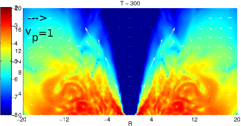
Figure 4.— The mass flux $\rho{\rm v}$ at T=300, in logarithmic color scale grading in units of $\dot{M}_{0}$, in a simulation without magnetic field. There is no significant mass or angular momentum flow after the relaxation phase. Vectors show the velocity of matter, with unit velocity in code units indicated in black arrow. The disk reaches the stellar surface, where matter is accreted onto the star.

Table 2Parameters used in our setups presented here. The initial inner disk radius is located at R${}_{\mathrm{i}}=10R_{\ast}$. The stellar rotation rate is $\Omega_{\ast}=0.15$, so that the corotation radius $R_{c}=3.54R_{0}=10.13R_{\ast}$. Shown are values for $B_{\ast}$ in the case of disk accretion rate $10^{-6}M_{\odot}$ yr^-1.

	S0	S1a	S1b	S2
$\kappa$	$10^{4}$	$10^{4}$	$10^{5}$	$10^{4}$
MA,0	$\infty$	274	35	223
$\delta_{0}$	100	500	50	100
$B_{\ast}$	0	24	190	30

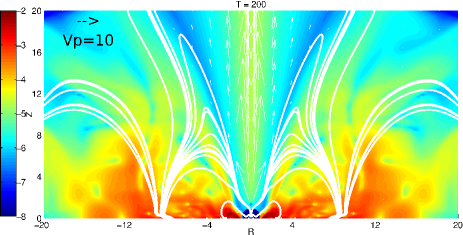
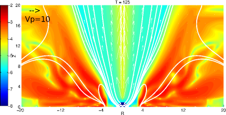
Figure 5.— The mass flux $\rho{\rm v}$ for the case with medium magnetic field in the simulation S1a is shown in the Left panel, and in the simulation S1b, with larger magnetic field, in the Right panel. Flow inside R$<0.5$ from the axis is very fast and light, and is artificial, of numerical origin. Mass flux is shown in a logarithmic color grading in units of $\dot{M}_{0}$, vectors show the velocity of matter, with ${\rm v}_{\rm p}=10$ in code units indicated in black arrow. The white solid line show the poloidal magnetic field lines. In both plots magnetic field lines nearby the axis are removed from the shown sample, not to obscure the underlying mass flux distribution. The disk is truncated at the radius where its ram pressure and magnetic pressure are balanced. In the case of simulation S1a this line is close to the stellar surface, so that in our resolution the disk almost touches the star. In simulation S1b the gap is well defined.

The electrical resistivity $\eta$ is defined through the electric conductivity $\sigma$ as $\eta=c^{2}/4\pi\sigma$, where $c$ is the speed of light. The ratio of the advection and diffusion terms in the induction equation (3) is the magnetic Reynolds number Rm=VL/$\eta$, where V and L stand for the characteristic speed and distance, respectively. The characteristic speed in our problem is the Alfvén speed ${\mathrm{v}_{A}}={\mathrm{B}}/(4\pi\rho)^{1/2}$, which defines the Lundquist number S_L.:

$$S_{L}=\frac{{\mathrm{v}_{\mathrm{A}}}L}{\eta}\,.$$ (18)

To explain the physical processes, the accretion disk requires an enhanced, anomalous level of resistivity, which is much larger than the classical value. The anomalous resistivity could be an effect of MHD turbulence or ambipolar diffusion in a partially ionized medium. We set the initial constant resistivity of the disk to be of the same order of magnitude as the numerical resistivity $\tilde{\eta}=\Delta x^{2}/\Delta t\sim 10^{-4}$, which gives $S_{\mathrm{L}}\sim 10^{4}$. We find the numerical resistivity by lowering the disk constant resistivity in the code until it does not affect the results.

We omit the actual Ohmic term in the calculation of the MHD equations. When the Ohmic part is included in the internal energy equation in Zeus347, Equation 4 gains an additional Ohmic heating term $-\eta\mathchoice{\mbox{\boldmath$\displaystyle j$}}{\mbox{\boldmath$\textstyle j$}}{\mbox{\boldmath$\scriptstyle j$}}{\mbox{\boldmath$\scriptscriptstyle j$}}^{2}$. The inclusion of this term is expensive computationally. However, the actual difference from the solution without the Ohmic term is negligible, as the $p\nabla$v term is much larger. Similar results have been reported in Miller & Stone (1997) and Romanova et al. (2009). It would take the Ohmic term many orders of magnitude larger to produce a visible effect.

A resistive corona is essential for the magnetic reconnection to occur, and reconnection is crucial for re-organizing the magnetic field. The resistivity is modeled as a function of matter density, following Fendt & Čemeljić (2002), so that $\eta\propto v_{\rm A}R\sim\rho^{(\gamma-1)/2}$. It comes from taking the turbulent velocity $v_{T}$ as a characteristic velocity in parametrization of resistivity, so that the resistivity is $\eta\sim v_{T}L$. Turbulent beta plasma is then $\beta_{T}=(c_{s}/v_{T})^{2}$, which gives $v_{T}=(\gamma/\rho\beta_{T})^{1/2}$, and the normalized turbulent velocity is then proportional to $\rho^{\prime(\gamma-1)/2}$. For the adiabatic case, $\gamma=5/3$ and $v_{T}\propto\rho^{\prime 1/3}$. Inserted back to the relation for $\eta$, this gives

$$\eta=\eta_{0}\ \rho^{1/3}\,.$$ (19)

To avoid unrealistically large $\eta$ and too small Ohmic timesteps $\tau_{\eta}=min(L^{2}/\eta)$ in the densest part of the domain, we limit this value to the order of unity, with $\eta_{0}=3.0$. Another restriction we imposed on the change of resistivity in each point of the computational box is that we do not allow it to be too steep. If in two succeeding instants of time the ratio of the new to the old resistivity is more than order of magnitude, we keep the old value of resistivity. It accounts for difference in the timescales for change of density and resistivity.

Another diffusive process in our simulations is the numerical viscosity. In finite differencing numerical scheme, it is of the same order as numerical resistivity. We do not treat the physical viscosity, only the von Neumann-Richtmyer artificial viscosity is included, through a constant parameter that controls the number of zones through which shocks are smoothed out. Such viscous term exists only in presence of shocks. For a smooth flow, it is tiny, and for rarefactions, it is zero. The characteristic speed for viscous effects is the sound speed $c_{\mathrm{s}}$.

In Table 2 we give parameters used for initial conditions in each of our presented simulations.

3. Results of simulations

Figure 6.— In the Left Panel is shown the density along the disk equatorial plane in simulations S1a and S1b at T=200 and T=125 in dotted and dashed lines, respectively. The initial density profile is shown in solid line. In the Right panel are shown the velocity profiles along the outer Z-boundary in the simulations S1a and S1b at T=200 and T=125, in the solid and dashed lines, respectively, in units of v${}_{\mathrm{K},0}=164~{}$km s${}^{-}1$. In the same simulations, Alfvén velocity is of the order of 10 v_K,0, escape velocity is of the order of 0.1 v_K,0, and sound speed is of the order of v_K,0.

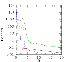
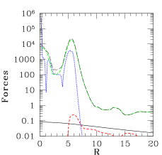
Figure 7.— In the Left and Right panels we show forces along the slice parallel to the disk equator, in simulations S1a and S1b, respectively, in a logarithmic scale. Slice is taken at half of the computational box, at Z=10; similar result is obtained all along the Z-axis. In blue dotted line is shown magnetic force, and in solid, green dot-dashed, red short-dashed and black long-dashed lines are shown absolute value of the gravitational force, pressure gradient, centrifugal and total forces, respectively. Ejection along the axis is artificial, produced by the steep gradient in magnetic pressure nearby the axis. At larger radial distance, realistic, physical ejections occur, and they are mainly launched by pressure gradient and magnetic forces.

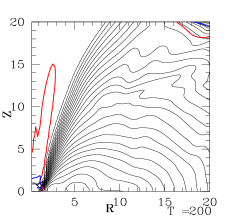
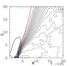
Figure 8.— Density isocontours in simulations S1a and S1b are shown in black solid lines in the Left and Right panels, respectively. In the left panel 25 isocontour lines are spanning logarithmically from $0.23\rho_{0}$ to $8.3\times 10^{-7}\rho_{0}$, along a line parallel to the axis of symmetry at R=10 from the disk equator to outer-Z boundary. In the right panel isocontour lines span the same way from $0.02\rho_{0}$ to $1.2\times 10^{-6}\rho_{0}$. Lines where $\beta$ and $\beta_{1}$ equal unity are shown in thick red and blue solid lines, respectively.

We started with a disk in hydrostatic balance and, as a reference, performed a hydrodynamic simulation without magnetic field. The stellar rotation rate in the case shown in Figure 4 was set to $\Omega_{\ast}=0.15$, but we tried smaller and larger values, with the similar outcomes. After relaxation, the disk remained stable for hundreds of revolutions, in a quasi-stationary state, connected to the stellar equator, with the matter from the disk very slowly falling onto the star. The disk got puffed up, similar to the situation in Čemeljić & Fendt (2004), where there was no central object in the simulation, only the disk. The reason for increase in the disk height is an increase in the pressure gradient force in the axial direction throughout the disk. It is an outcome of a slight heating-up of the disk in our simulation with $\gamma=5/3$. In simulation with smaller $\gamma<4/3$, disk puffs-up less. However, for reasons of easier comparison with other works, we decided to keep $\gamma=5/3$ in our simulations here.

3.1. Simulations with very small and with small magnetic field

We seek to understand the effects of magnetic diffusion on the launching of matter from the innermost vicinity of an YSO. In our code, numerical resistivity and numerical viscosity are of the similar order of magnitude. By including physical resistivity, but not physical viscosity, we probe the portion of parameter space with $Pr_{\mathrm{m}}<1$. The stellar rotation rate remains $\Omega_{\ast}=0.15$, the same as in the case without the magnetic field.

At very small pure stellar dipole magnetic field, of the order of 0.1 G, we notice that very fast flow occurs above the star close to the axis, carrying very small mass flux. Similar solutions are obtained until we reach the stellar dipole magnetic field of the order of 10 Gauss, for an YSO disk accretion rate of $10^{-6}M_{\odot}$ yr^-1. At this field strength, in addition to the flow above the star close to the axis, a slower ejection of matter at larger angle from the axis, occurs.

We check in more detail this solution with medium magnetic field, of the order of 10 Gauss, which we name simulation S1a. The field is not strong enough to completely terminate the disk, which is still falling radially onto the star with a very small velocity of 0.1v${}_{\mathrm{K},0}\sim 16.4$ km s^-1. It is possible that our resolution is insufficient for establishing the inner disk radius, as the line of balance of gas and magnetic pressure is very close to the stellar surface. The final state in simulation S1a is shown in Figure 5. In the flow very close to the axis of symmetry, velocity is reaching the order of few hundreds of v_K,0, and at around 1/4 of the R_max from the axis, velocity reaches the order of few tens of $v_{\mathrm{K},0}$, (see Figure 6), which gives $1.6\times 10^{3}km~{}s^{-1}$ in the YSO case). Other characteristic velocities, like sound speed and Alfvén velocity, are all much smaller than the Z-component of velocity, which is the main contributor to total velocity shown by arrows in Figure 5.

3.2. Artificial axial flow

Inspection of forces in the radial direction, shown in Figure 7, shows that axial ejection is of numerical origin, produced by an unrealistically large magnetic force. This force is produced by the large gradient of magnetic pressure along the axis, which decreases inversely proportional to the radial distance $R$. That the axial ejection is artificial, follows also from the observation that it appears in runs with very small magnetic field. It is not the case with the ejection at larger angle: it appears only when magnetic field is above some critical value, which is of the order of 10 Gauss. Further from the axis, magnetic force contributes to the launching, but is always smaller than the pressure gradient force.

We try to prevent formation of this artificial axial flow choosing different density floors, but they hamper evolution of the system through the violent relaxation, and simulations stop or become unphysical – with density governed by the density floor. Another method would be to add outflowing gas from the stellar pole, but it is overcome by the strong artificial magnetic field, and axial flow anyway appears. Since this flow is easily discernible from other flows as being generated by numerically obtained magnetic force, we decided to leave it, as a numerical effect in the simulations.

3.3. Simulations with larger magnetic field

Figure 9.— In solid line are shown mass fluxes F_m, and in dashed line the angular momentum fluxes F_l in the simulation S1a (Left panel) and S1b (Right panel), at T=200 and T=125, respectively. Slices are taken along the outer Z-boundary. Fluxes are calculated for only the 1/3 of R_max part of the box, where ejection occurs. Note the different scales at the left and right side of plots.

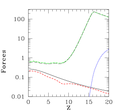
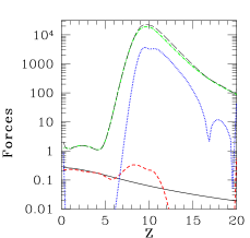
Figure 10.— Forces in simulation S1a at T=200 (Left panel) and S1b at T=125 (Right panel), in a logarithmic scale. In black solid, green dot-dashed, red short-dashed, blue dotted and black long-dashed lines are shown absolute value of the gravitational force, pressure gradient, centrifugal, magnetic and total forces, respectively. Forces are taken along slices parallel to the axis of symmetry, at R=5.

With increase in magnetic field for an order of magnitude in comparison to the field in simulation S1a, the disk terminates at a line where the magnetic and ram pressure are equal (Figure 8). At this line the plasma $\beta$ parameter, which is the ratio of the gas and magnetic pressure $\beta=8\pi p/B^{2}$, equals unity. In the same Figure we also draw the line where the parameter $\beta_{1}=8\pi(p^{2}+\rho v^{2})/B^{2}$ equals unity. The flow is magnetically dominated when one of those parameters becomes less than unity. Now there is no radial infall onto the star any more. We name this simulation S1b. In Figure 6 we show the velocities in the launched matter. The part of the outflow nearby the axis is a numerical effect, as in simulation S1a, produced solely by the magnetic force, shown in Figure 7. The slower flow, launched by the combination of pressure gradient and magnetic forces, is now launched at a larger angle than in simulation S1a.

We calculate the mass flux F_m and the angular momentum flux F_ℓ in each half-plane, above or below the disk equator. They are defined as:

$$F_{\mathrm{m}}=\int_{0}^{R}2\pi\rho{\mathrm{v}}_{Z}RdR\ ,$$

$$\quad F_{\ell}=\int_{0}^{R}2\pi\left(\rho{\mathrm{v}}_{Z}{\mathrm{v}}_{\phi}R-\frac{B_{Z}B_{\phi}R}{4\pi}\right)dR\ .$$ (20)

In Figure 9 is shown radial distribution of flux in simulations S1a and S1b in the first 1/3 of $R_{\mathrm{m}ax}$. Both fluxes are very small, with the mass flux of the order of $10^{-6}\dot{M}_{0}$, for a few orders of magnitude smaller than the estimate in the optical jets from observations, usually inferred to be 10% of the disk accretion rate. Mass and angular momentum fluxes from the artificial flow closest to the axis (for $R<0.5$) contribute very little to the total fluxes, as they are even an order of magnitude smaller. From Figure 9 we read that maximum of ejection in simulation S1a occurs under an angle of $\Theta=3^{\circ}$ from the axis, and drops steeply to half of the peak value until $\Theta=9^{\circ}$ from the axis. In the simulation S1b, matter is launched into a wider angle, from $\Theta=3^{\circ}$ to $\Theta=20^{\circ}$.

Which force is launching the matter above the disk gap? In Figure 10 we show forces along the ejecta. The force exerted because of the pressure gradient is contributing significantly to the total force. Hence, fast, but very light ejection of matter in our simulation is driven by a combination of pressure gradient and magnetic forces. Ejection is directed outwards from the star-disk system, in presence of ongoing magnetic reconnection along the boundary between the stellar and disk components of the magnetic field. Matter from the corona is launched along this boundary layer, so that reconnection is pushing the ejecta along the current sheet which is established at the boundary. Our disk is puffed-up; it is probable that for thinner disk in simulations the angle of ejecta would be larger, as then magnetic field higher above the gap would be less pressed towards the axis by the disk. The ejected matter, which originates from the corona, and not directly from the disk, is very fast and light, as shown in Figures 6 and 9. This is the main difference of our result with results from the Table 1.

Because of role of reconnection in launching, our results are similar to situation in solar context, when micro-flares are launched into a solar corona, only that in our case matter is launched from the magnetosphere between the star and the disk. To distinguish our ejections from other cases of more massive outflows in the star-disk system, we name them micro-ejections, as they are tiny in mass flux, and localized nearby the boundary between the stellar and the disk magnetic field. Position of our micro-ejections seems to suggest that magnetic field producing them could have similar geometry as a helmet streamer in X-wind model (Shu et al., 1994).

Varying the accretion rate and strength of the magnetic field does not change the nature of our result: micro-ejections remain light and fast.

What is the reason for launching under a wider angle? Is it because of larger magnetic field, or conditions near the disk gap? Forces along the flow in Figure 10 show that the reason for launching is the same, only with much larger pressure gradient force in simulation S1b. Mass and angular momentum fluxes remain very small, but above the value which could be set by the density floor, set in our simulations to $5\times 10^{-8}$ in code units. The axial region remains almost evacuated because of the fast ejections, which have a tiny mass and angular momentum flux.

In a setup as described, simulations with larger magnetic field, of the order of kG, tend to stop during, or not long after, the relaxation, because of numerical problems. To study the quasi-stationary state, in which small fluxes we obtain could evolve further (and eventually increase or disappear), simulations lasting for hundreds of rotations are needed, with a stable disk gap and realistic magnetic field strength.

3.4. Long-lasting simulations with fixed disk gap

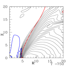
Figure 11.— In the Left panel is shown change in time of the disk density profile in simulation S2 along the equatorial plane. We show densities at T=0,5,10,100,850 in thin solid, dotted, dashed, long dashed and thick solid line, respectively. The disk density is substantially modified only during the relaxation, afterwards it does not change much. In the Right panel are shown density isocontours at T=750 in black solid lines, in 25 logarithmically spanning lines along the line parallel to the axis of symmetry, ranging from $0.11\rho_{0}$ at R=10 in the equatorial plane of the disk, towards $5\times 10^{-8}\rho_{0}$ at the outer-Z boundary. Positions where $\beta$ and $\beta_{1}$ are unity shown in thick red and blue solid lines, respectively.

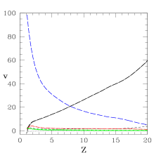
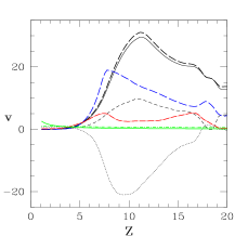
Figure 12.— Velocity profiles in simulation S2, in units of v${}_{\mathrm{K},0}=164~{}$km s${}^{-}1$, for results from the bottom panel in Figure 14 at T=750. Profiles along the propagation direction of micro-ejection in the Z-direction, parallel to the symmetry axis, at $R=R_{\ast}$ we show in the Left panel, and at a larger distance $R=5R_{\ast}$ in the Right panel. Components of the velocity in Z, R and toroidal direction are shown in thin solid, dashed and dotted black lines, respectively. Poloidal, Alfvén, escape velocity and sound speed velocities are plotted in the long-dashed (black), long-dashed (blue), dot-short-dashed (green) and dot-long-dashed (red) line, respectively.

Figure 13.— In solid line is shown mass flux F_m in units of $\dot{M}_{0}$, and in dashed line the angular momentum flux F_l in the corresponding units in the simulation S2 at T=750. Scales from the left and right side of the plot are for F_m and F_l, respectively. Slices are taken along the outer Z-boundary. We show the fluxes only for part of the box where the micro-ejection is located.

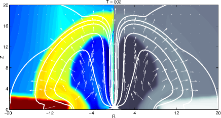
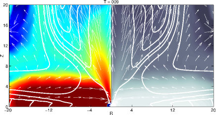
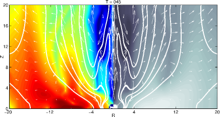
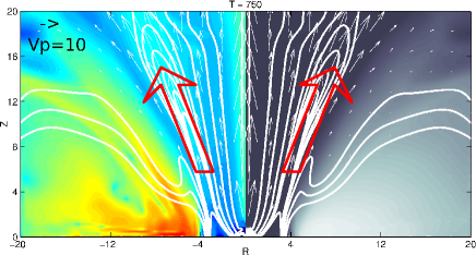
Figure 14.— Snapshots in our simulation S2. The left half of each panel shows the poloidal mass flux $\rho{\rm v_{p}}$, and the right half shows the density. Lines and arrows have the same meaning as in Figure 5. Both plots are in logarithmic color scales, shown at the bottom of the panels, with mass flux in units of $\dot{M}_{0}$ and density in units of $\rho_{0}$. The initial magnetic field is a pure stellar magnetic dipole, with value $B_{\ast}=30$ G if assumed disk accretion rate is $10^{-6}M_{\odot}/$yr^-1. Top to bottom are shown characteristic stages discussed in this work: I) initial relaxation when the magnetic field is swept in and pinched near the disk mid-plane toward the star, II) inflation and reconnection that end up opening the field, and strong infall of matter onto the star from the disk, III) retraction of the disk matter towards the corotation radius, with a transient inflow of matter onto the star, and the light bullets of fast matter expelled along the axis-which is a numerical, artificial flow, IV) final, quasi-stationary stage, with a light, fast micro-ejection launched along the boundary layer between the stellar and the disk field. For clarity, we additionally marked micro-ejection with large red arrows.

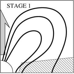
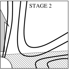
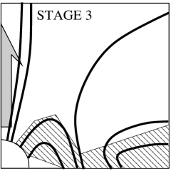
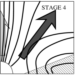
Figure 15.— A schematic sketch of the evolution in star-disk interaction in our simulations. Stage one: the initial stellar dipole gets pinched during the relaxation, when matter flushes in toward the central star; Stage two: the magnetic field lines are open after reconnection, and disk matter can reach the surface of the star. Our simulations here differ from most of the works in Table 1 in the violent initial conditions which bring the disk onto the star. For the setups with a stable disk, such situation occurs only in the regime of very weak stellar magnetic field. In the case of strong magnetic field, configurations will be as sketched in Goodson et al. (1999), where the disk terminates in the magnetosphere, away from the star; Stage three: the disk matter retracts and a funnel flow forms from the disk inner radius and accretes matter onto the star; Stage four: the system reaches a quasi-steady state, with magnetic field re-organized into a configuration consisting of an open stellar field and field footed in the disk. The arrows indicate the directions of the matter flow. In the first three stages, artificial flow of a numerical origin forms (marked with gray shadow) along the axis. It is of negligible mass flux. In the fourth stage, along the boundary between the stellar and the disk magnetic field, launched is a micro-ejection, which reaches a quasi-stationary state (marked with black shadowed arrow) together with magnetic field.

To obtain longer lasting simulation, we devise a simulation with the disk gap numerically imposed, as described in §2.2. Such simulation, dubbed S2 here, has been performed with a part of the disk mid-plane inside the disk gap defined as an open boundary. It means that the disk truncation radius is not determined self-consistently. For a changed boundary condition, we check the change of density in time along the disk equatorial plane in Figure 11. Inflow of matter into the disk from the outer boundary, which mimics the accretion of matter from the outer part of the accretion disk, has to be well chosen. In the case of a too large inflow of matter into the disk, it would pile up and the disk would become unstable. On the other side, if the disk would become drained of matter, it would change the conditions we want to investigate. In Figure 11, we see that after the relaxation, our reservoir of matter in the simulation is not changing for too much. In the other panel of the same Figure we show lines along which parameters $\beta$ and $\beta_{1}$ equal unity, marking positions where the flow becomes magnetically dominated. For our purpose of obtaining simulation similar to S1b, it is important that those lines are similarly positioned in both simulations.

Snapshots at different times in simulation S2 are shown in Figure 14. We show the density and poloidal mass flux $\rho{\rm v_{p}}$ for the same time step in the right and left side of the same panel, to stress that in the density plots micro-ejection will typically not be visible even in logarithmic color grading. Other features, as ejected plasmoid or accretion flow onto the star are well seen in both the density and mass flux plots, and have been described in the literature mentioned in §1. Micro-ejections which we report here are lighter, so that they are not easy to contrast even in logarithmic plots with mass fluxes.

We show the velocity along the micro-ejection in the quasi-stationary state in Figure 12. The flow is supersonic and sub-Alfvénic close to the stellar surface, but at the middle of the computational box it becomes super-Alfvénic. Both the poloidal and total velocity in micro-ejection are larger than the escape velocity $v_{\mathrm{e}sc}=(2GM_{*}/R)^{1/2}$. The total velocity is for two orders of magnitude larger than the escape velocity. In Figure 13 we show the radial dependence of fluxes $F_{\mathrm{m}}$ and $F_{\ell}$ across the outer Z-boundary in the quasi-stationary state.

Now we obtained a long lasting simulation, which resembles S1b, but the magnetic field required for the launching of micro-ejection is smaller for almost an order of magnitude. We can identify four evolutionary stages in progression in a system of an interacting magnetosphere with its surrounding disk. We show snapshots taken at different times, in Figure 14. The time-evolution proceeds in the similar way in simulations S1a and S1b, and the results are robust in that they occur under a wide range of explored parameters, although each with different details. An initially pure dipole magnetosphere has already bulged out and brought some gas along with it at as few rotations as $T=2$. Near the axis, some gas also flows out at high velocity due to magnetic pressure that is gradually building up–because of unrealistic large magnetic force there, we conclude that this flow is artificial, of numerical origin. The matter in the disk has flown in at a magnetic stagnation point around $8R_{\ast}$, where the magnetic field dragged in with the gas is pinched. Around $T=9$, matter went through a magnetic reconnection and ejected plasmoids. The reconnected and opened field enabled the disk gas to flush into the stellar surface and, at the same time, more violent gas flows are directed outwards both from the axial region and from the disk. At a later time, $T=45$, after a few occurrences of the magnetic reconnection events, part of the field closes back to the stellar surface, and part remains open, footed near the new truncation radius, which is in this case pre-determined by the boundary conditions. Matter channels through the field lines that are footed both in the disk and the stellar surface. Matter along the axis is still expelled by a numerical effect, in the form of bullets or, when more stabilized, in a more continuous light, very fast stream. The bottom panel in Figure 14 shows the representative snapshot in this simulation at a much later time $T=750$. The system settled into a configuration where the magnetic field has been opened into space with either foot in the star or in the disk, and formed loops that connect to both the star and the disk. The gas flows out from the regions on top of the star in an artificial fast flow, and from the boundary on top of the loops along the diverging field lines open to the space, forming micro-ejection. The matter which is launched outwards originates from the magnetosphere above the disk where one foot of the magnetic field is rooted. The mass and angular momentum fluxes in the artificial, axial flow are typically for at least one order of magnitude smaller than in micro-ejection launched under larger angle. The disk material stays slightly outside of the magnetic footpoint where the field is pinched, around the truncation radius. The disk, after the relaxation, does not differ much from the purely hydrodynamic case in Figure 4.

Similar steps have been observed in other simulations with violent relaxation, as e.g. (Goodson & Winglee, 1999). This process can be described by four conceptual stages, shown in a schematic sketch in Figure 15. Stage I is the initial relaxation from the highly non-equilibrium state in our simulation, when the magnetic field is swept in by matter infalling from the disk towards the star, and pinched near the disk mid-plane. The magnetic loops are twisted, inflating and forming plasmoids. The gas that flows with the field swirls in and is gradually accelerated in the axial region by magnetic pressure being built up. Stage II takes the scene after the system goes through a reconnection that ends up opening the field, enabling strong infall of matter onto the star from the disk. The artificial axial flow, steady or in a series of bullets, forms as a result of magnetic pressure from the twisted field, built because of numerical effect nearby the axis. Stage III follows when the disk matter retracts towards the corotation radius, and a time-variable inflow of matter funnels onto the star from the inner disk truncation radius. The system may have several passages through the first three stages and finally move onto the quasi-steady state when the magnetic field is pinched and strong enough to balance the ram pressure of the disk gas, truncating the disk near the magnetospheric radius. The magnetic field settles into a geometry where the field is open into the space both axially and conically, with some loops anchoring both in the star and the disk. Matter flows out quasi-stationary along the open field lines, forming the fast micro-ejection along the current sheet formed between the disk and the stellar component of the magnetic field.

Evolution should proceed in a similar way for simulations with slowly rotating star which, as ours, start with non-equilibrium initial conditions and with not too strong stellar magnetic field, with disk reaching the star during the violent relaxation phase. If the disk retracts is depending of the strength of magnetic field: for a small field, the gap does not form. For a sufficient large field, the disk is truncated, and a disk gap is formed.

4. Properties of micro-ejections

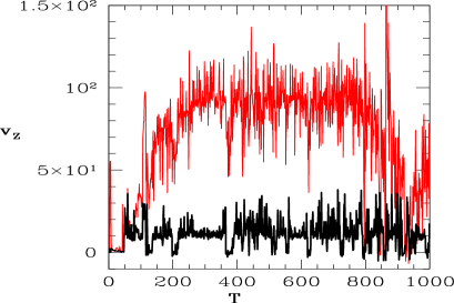
Figure 16.— Velocity in the axial direction in simulation S2, throughout the simulation. We show the velocity in the micro-ejection at $(R,Z)=(0.4R\ast,Z_{\mathrm{m}ax})$ in a thin (red) solid line, and in at $(R,Z)=(7.1R_{\ast},Z_{\mathrm{m}ax})$ in a thick (black) solid line. In the former case average value in the quasi-stationary state is of the order of 80v_K,0, and in the latter it is of the order of 10v_K,0.

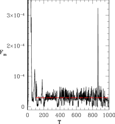
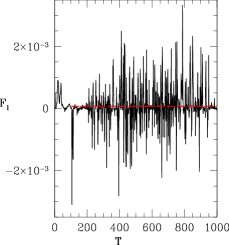
Figure 17.— Time evolution of mass (Left panel) and angular momentum (Right panel) fluxes in simulation S2, parallel to the axis of rotation, along the ${\mathrm{Z}_{max}}$ boundary for 1/3 $R_{\mathrm{m}ax}$ part of the box. We show the fluxes after the relaxation in solid (black) line. In dashed (red) line we show the average value, computed starting from T=100, when the flow becomes quasi-stationary. The mass flux average value is $3.0\times 10^{-5}\dot{M}_{0}$, and the angular momentum flux average value is $7.4\times 10^{-5}$.

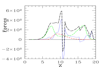
Figure 18.— Forces in simulation S2 at T=750 along slice parallel to the axis of symmetry, at R=5. In black solid, green dot-dashed, red short-dashed, blue dotted and black long-dashed lines are shown gravitational, pressure gradient, centrifugal, magnetic and total forces, respectively. Micro-ejection is driven by a combination of pressure gradient and magnetic forces.

Figure 19.— Average mass and angular momentum fluxes F_m and $F_{\ell}$ in our simulations with changing density contrast $\kappa$ between the disk and the corona are shown in the Left panel, and with changing stellar magnetic field strength in the Right panel. In solutions with $\kappa=(10^{2},10^{3},10^{4},10^{5},10^{6})$ we show the mass flux in solid line, and the angular momentum flux in dashed line. Results for the mass flux for $\kappa=10^{2}$ in our simulations are always larger for a factor of 2 to 3, than for larger, more realistic values of $\kappa$. In simulations with increasing magnetic field, we show the mass flux in units of $\dot{M}_{0}$ in solid line, and the angular momentum flux in the corresponding units in dashed line. With stellar magnetic field $B_{\ast}=(3,10,30,77,188)G$, with disk accretion rate $10^{-6}M_{\odot}/$year, both fluxes increase with increasing magnetic field. If we assume $10^{-8}M_{\odot}/$year, magnetic field strenghts are 1/10 of those values.

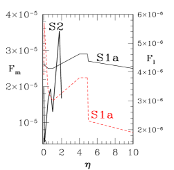
Figure 20.— In the Left panel we show change of mass flux with variation of stellar rotation rate $\Omega_{\ast}$. Mass flux in micro-ejection increases with increasing $\Omega_{\ast}$. In the Right panel we show average mass fluxes F_m in simulations S1a and S2 in dependence of maximum resistivity in the computational box (the numerical resistivity is included). Mass fluxes are shown in thick and thin (black) solid lines, respectively. The average angular momentum flux F_l in simulation S1a and its dependence on resistivity is shown in the dashed (red) line. We do not show result for angular momentum flux for simulation S2, as it varies randomly between $-10^{-6}$ and $10^{-6}$. Values for both fluxes in simulation S1a for $\eta=50$ are not shown in the figure, but are similar to values for $\eta=10$. Note the different labels in the left and right sides of the plot.

Here, we describe in more detail the properties of matter in micro-ejection in the quasi-stationary solution in our simulation S2. In Figure 16 we show the change of velocity in chosen points in the computational domain. Oscillations show a sign of instability working at a short time scale, so that the flow in micro-ejection varies even in the quasi-stationary phase. The reason is that magnetic field is permanently reshaped by reconnections along the flow — we discuss it in more detail in §5. In Figure 17 we show the time evolution of those fluxes. To avoid influence of the disk flaring in presenting the results, we integrate fluxes only to $R_{\mathrm{m}ax}/2$ at each time step. The fluxes reach quasi-stationarity after relaxation and stabilization of the system. Reconnection events along the boundary layer between the stellar and the disk fields contribute to the oscillation at the timescale of one rotation period. Following the evolution of ejections longer into the quasi-stationary phase, we measure that the contribution to the total fluxes from the artificial flow very close to the axis is at least one order of magnitude smaller than from the ejections launched under larger angle.

Forces along micro-ejection, in a slice parallel to the axis at R=5, are shown in Figure 18. The same as in simulations S1a and S1b, the combination of pressure gradient and magnetic forces is driving a micro-ejection.

4.1. Dependence of results on the density contrast, magnetic field, stellar rotation rate and resistivity

Simulations in the literature, as we show in Table 1, were performed for various contrasts of the disk to corona density $\kappa$. What is the influence of this parameter in our simulations?

We show results for variation of this parameter in simulations set-up like simulation S2 in Figure 19. There are no significant differences in the average fluxes in the range of $\kappa$ from $10^{3}$ to $10^{6}$. For $\kappa=10^{2}$, the mass flux is always larger, so that it is double or, in some setups, triple the value from other cases. We checked that this trend, which is illustrated here for a case of sub-Keplerian rotation of the disk, is true also in the case of Keplerian rotation profile. This means that results of simulations with $\kappa=10^{2}$ could be unrealistic in the case of launching of astrophysical outflows. This is not surprising, taking into account that the realistic value of $\kappa$ is probably somewhere between $10^{8}$ and $10^{5}$ for YSOs-this value will inevitably strongly depend on local conditions.

We also check how the mass flux in simulation S2 depends on the magnetic field strength. In Figure 19 are shown the average fluxes for magnetic fields up to 200 G, for YSOs with a disk mass accretion rate of $10^{-6}M_{\odot}$ yr^-1. Both the mass and angular momentum fluxes increase with increasing magnetic field strengths. Our fluxes are very small, as the source of matter is magnetosphere above the gap, and not directly the disk surface. Simulations like those from the Table 1 with stellar fields of about 1 kG may truncate the disks and launch stable, massive outflows, with the matter from the disk inner radius.

Our simulations are performed for slow stellar rotation. We check how fluxes change with variation of stellar rotation rate $\Omega_{\ast}$. Results for mass fluxes are shown in Figure 20, for $\Omega_{\ast}=$0.068, 0.1 and 0.15, which correspond to corotation radii 6.0R₀, 4.6R₀ and 3.5R₀, respectively. Mass flux increases with increasing stellar rotation rate, i.e. decreases with increasing corotation radius. Angular momentum fluxes do not show clear dependence.

Because of violent relaxation, a simulation can fail at early stages, so that it is not easy to perform a parameter study of dependence on resistivity. Each of the runs has its preferred level of resistivity, to last for for hundreds of rotations into the quasi-stationary state. We choose S2 as a representative case because it lasted more than 500 Keplerian rotations at $R_{0}$ with unit maximum resistivity. In Figure 20 we show that average mass and angular momentum fluxes do not depend on resistivity. For comparison, and to show that the same is true also in the case of self-consistent disk gap boundary, we show along also the mass flux in simulation S1a – in both cases variation remains small, within the same order of magnitude. With larger magnetic field in simulation S1b, it is difficult to obtain quasi-stationary results for a range of values of resistivity, so that we do not provide values for simulations in S1b. Resulting fluxes could depend on the model of resistivity, as it will enable or prevent reconnection to occur. In simulations with higher resolution than in our simulations here, this dependence could be more visible, as then the numerical resistivity triggers with the lower value, leaving larger portion of the parameter space for the physical resistivity.

5. Reconnection and opening of magnetic field lines

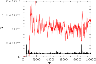
Figure 21.— Change of resistivity with time in simulation S2, in units of $\eta_{0}=10^{19}$cm² s^-1. We show $\eta$ in two positions (R,Z) in the computational box: at the exit region of the micro-ejection in the position (7,$Z_{\mathrm{m}ax}$), and in the middle of the computational box, in the position (10,10), in thick (black) and thin (red) solid lines, respectively. As expected in our model with resistivity in the disk corona dependent on the density, closer to the disk, resistivity is larger.

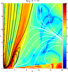
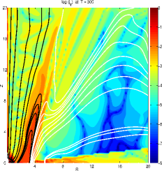
Figure 22.— In the Left panel is shown absolute value of the toroidal current $j_{\phi}$ at T=125 in simulation S1b, in logarithmic color grading, in code units. In solid lines are drawn poloidal magnetic field lines, with lines along which magnetic field vector points towards the star, painted in black color, and those where the field points in the opposite direction, in white color. Similar result is obtained in simulation S2 at T=300, as shown in the Right panel. Reconnection is ongoing along the boundary sheet throughout the quasi-stationary state, and pushes the matter out of the magnetosphere, in addition to the force caused by the pressure gradient. In the simulation S1a, such current sheet forms closer to the star and under smaller angle, measured from the axis.

Figure 23.— Isocontours of Lundquist number S_L in S1b, at T=125. Values of $S_{L}$ for some isocontours are labeled on the plot.

Reconnection is essential for launching outflows from a star-disk magnetosphere. If, for some reason, reconnection does not occur, a magnetic wall forms and the evolution of the system will be different. In the simulation with non-resistive corona, magnetic field does not relax in the same way as in the simulation with a resistive corona. Without resistivity, the corona relaxes from the initial condition with a steeper gradient between the stellar and the disk component of the magnetic field, because of slower reconnection process, as seen e.g. in Fendt (2009), where the disk was treated as a boundary condition, with resistivity included in a whole domain.

Resistivity facilitates the reconnection, and shape the geometry of the final magnetic field. Even if physical resistivity is not included in the code, there is unavoidable numerical resistivity, which can be estimated as $\eta_{\rm num}=v\Delta x$, where $\Delta x$ is the grid spacing and the characteristic velocity is the poloidal Alfvén velocity. As numerical resistivity is different from physical, results obtained with non-resistive code could be unphysical. On the other side, chosen physical model of resistivity can also affect the applicability of the results (Goodson et al., 1997).

We included physical resistivity in the code, modeled in dependence of the matter density, and allowed it to vary in time. In Figure 21 we show variation of resistivity with time in two positions in the computational box. Reconnection is ongoing along the boundary between the stellar and the disk magnetic field. The toroidal component of the current $j_{\phi}$ in Figure 22 shows the position of a current sheet in the computational box in the quasi-stationary state in the simulation S1b. The sheet forms close to the boundary line where the star and the disk fields, which are in our case of opposite direction, meet. Reconnection is ongoing along the boundary during the time-evolution, into the quasi-stationary state. It looks similar in simulation S2, and in simulation S1a a current sheet starts from the magnetosphere closer to the star. Reconnection pushes the matter outwards from the magnetosphere in the disk gap, in addition to the force caused by the pressure gradient and magnetic force. To show the spatial distribution of resistivity, we compute the Lundquist number S_L in the quasi-stationary state of simulation S1b, in the Figure 23, with labeled values for some isocontours of the value of S_L.

6. Elsasser criterion for launching

Launching by a magnetospheric accretion-ejection is the result of interaction of the magnetosphere and the innermost portion of the disk. In our setup, with the resistivity modeled by the density, line where the Lundquist number S${}_{L}=1$ shows to be useful indicator of the launching region, but this might be dependent on the model of resistivity. The best, and most general indicator is the line where the magnetic and matter pressure are equal ($\beta=1$).

Another number which we find to indicate where from the launching is possible, is the Elsasser number. It is defined by the ratio of the Z component of the Alfvén velocity and $\eta\Omega_{\rm K}$ (see Salmeron et al. (2007) and references therein):

$$\Lambda\equiv\frac{V_{\mathrm{A}Z}^{2}}{\eta\Omega_{\rm K}}>1\,.$$ (21)

In some systems, when the flow is mainly in the Z-direction, $\Lambda$ can be similar or equal to the Lundquist number S_L, or magnetic Reynolds number Rm, but in general they are different, because velocity of the outflow differs from the Alfvén velocity.

In Figure 24, we plot the Elsasser number $\Lambda>1$ in simulations S1b and S2. We observe that $\Lambda\geq 1$ is valid only in the magnetosphere above the disk. For a small magnetic field of the order of 1 G, there is no region in the box that could satisfy $\Lambda\geq 1$, and no launching is possible. For comparison, in the same figure we show the lines where the magnetic and matter pressure are equal ($\beta=1$), and where the Lundquist number equals unity. All three lines meet close to the disk inner radius-the same is the case in simulations S1a-but then separate higher above the disk. When compared with positions where ejection is present, the line where $\Lambda=1$ and S_L=1 gives the best separation between the locations where ejections do and do not occur, in the cases of weaker magnetic field. The reason is possibly in $\Omega_{\rm K}$ in the expression for $\Lambda$, which is still connecting it with the disk, even in description of the (non-Keplerian) corona. We will investigate this relation in further work, with more realistic disk. Line with $\beta=1$ is always correctly following positions with the strongest ejection.

7. Disk truncation radius

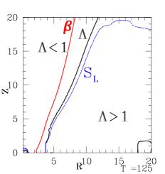
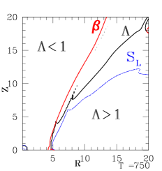
Figure 24.— In thick (black) solid line is shown Elsasser number $\Lambda$ at T=125 and T=750 in simulations S1b and S2, in the Left and Right panels, respectively. Above the line in the computational box where magnetic pressure equals matter pressure ($\beta=1$), and where the Elsasser number $\Lambda$ equals unity (red solid line), launching of a flow of matter is possible. Below those lines, the launching of matter can not occur. For comparison, we show also the line where the Lundquist number $S_{L}$ equals unity, in solid blue line.

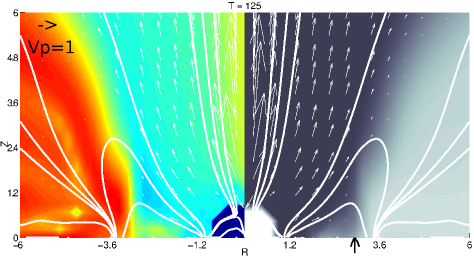
Figure 25.— A zoom into the closest vicinity of the star from Figure 5 in simulation S1b, to show details in the disk gap, where the disk is truncated. Meaning of colors and lines is the same as in Figure 14. The stellar magnetic field is about 200 G, for the disk mass accretion rate $10^{-6}M_{\odot}$ yr^-1. Black arrow marks the position of the truncation radius of the disk, which is in this case $R_{\mathrm{t}}=3.0R_{\ast}$.

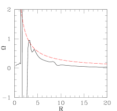
Figure 26.— In Left panel in solid line is shown angular velocity profile along the disk mid-plane at T=125 in simulation S1b. For comparison, in dashed (red) line we show a Keplerian rotation profile. In the Right panel we show, at the same time, components of velocity along the same plane: v_Z, v_R and v_ϕ in solid, dashed and dotted lines, respectively.

Figure 27.— Left panel shows poloidal, toroidal and total magnetic field along the disk mid-plane in simulation S1b at T=125 in dashed, dotted and solid lines, respectively. Ratio of gas and magnetic pressures along the same line is shown in the Right panel.

In simulation S1b we maintained self-consistent boundary conditions at the disk mid-plane, so we can try to estimate the disk truncation radius from our results. The new truncation radius of the disk after the relaxation is close to the line of balance of the disk ram pressure and the magnetic pressure, $p+\rho v^{2}=B^{2}/8\pi$, located between a central object and the disk inner radius. We show it in the §3.1, where in the right panel of Figure 8 we read that magnetic pressure is equal to the gas pressure at the distance of about R=2R_∗. To show details nearby the disk gap, in figure Figure 25 we zoom close to the star in simulation S1b. The disk terminates at $R_{\mathrm{t}}=3.0R_{\ast}$, close to the position where the disk density drops steeply, and where the magnetosonic Mach number equals unity at the equatorial plane, as matter is being launched fast along the neutral line because of reconnection. The angular velocity profiles along the disk mid-plane also show a dip at the disk truncation radii, passing from the gap into the disk, as shown in Figure 26. The magnetic field strength and the ratio between the gas and magnetic pressure are shown in Figure 27. All show steep gradient in quantities at crossing the disk truncation radius.

The disk truncation radius can be estimated as $R_{\mathrm{t}}=\alpha_{\mathrm{t}}(B_{\ast}^{4}R_{\ast}^{12}/2GM_{\ast}\dot{M}_{\rm a}^{2})^{1/7}$, given by order of magnitude as the equilibrium of the ram pressure of a spherical envelope in free fall and the magnetic pressure of a stellar dipole (Elsner & Lamb, 1977). The non-dimensional factor $\alpha_{\mathrm{t}}<1$ has been estimated to be 0.5 in Ghosh & Lamb (1978, 1979a, 1979b) and $\sim 1$ in Ostriker & Shu (1995). In our simulations the system departs significantly from the spherical infall case and results in too large $\alpha_{\mathrm{t}}$, when compared to the estimate above. Simulation S1b yields $\alpha_{\mathrm{t}}=4.17$. Simulations in better resolution might improve matching with the theoretical prediction.

Bessolaz et al. (2008) estimate $\alpha_{\mathrm{t}}$ to be equal to $M_{s}^{2/7}$, where $M_{s}$ is the sonic Mach number measured at the disk mid-plane, using the radial velocity of the matter in the disk for a comparison with the sound speed. Their derivation was for the case with the accretion column onto the star, but conditions should be similar also in the case of ejection launched from the inner disk radius. For this estimate, inserting the values from simulation S1b, we obtain $M_{s}^{2/7}=0.15$, which gives a $R_{\mathrm{t}}=0.3R_{\ast}$. None of the two estimates matches our result here. The reason is probably in disk puffing-up because of heating produced in the disk, in our simulation with $\gamma=5/3$. An investigation of location and stability of the disk truncation radius should be done in a simulation with better disk computation. Further improvement would also be to perform simulations in the complete R-Z half-plane, to remove the constraint by the disk equatorial plane boundary condition.

8. Discussion

In this work, we for the first time demonstrate launching fast, light quasi-stationary flows of matter, which we call micro-ejections, from the magnetosphere above the gap in the star-disk system. In our simulations we included physical resistivity not only in the disk, but in the whole computational box. We investigate effects of anomalously large resistivity (when compared to microscopic resistivity), modeled as a function of matter density, to the launching of such micro-ejections in the case of slowly rotating star.

The physical resistivity, when included in previous simulations in the literature, was limited to the disk, decreasing effectively to zero out of it. The reconnection above the disk, which is necessarily happening during such simulations, was at the mercy of numerical resistivity, whose effects are different from physical resistivity In order to better understand differences between a variety of setups, we compare resistive simulations performed to date — some of them are shown in Table 1. Resistivity can only moderately modify the flow shape, on a slower time scale than the formation of a magnetic wall (Lynden-Bell, 1996, 2003), so that if the resistivity is not large enough for reconnection to occur, the geometry of the flow will be different. As sketched in Figure 15, common phenomena have been identified in our simulations, which occur, in those simulations of interacting star-disk systems from Table 1 which have violent initial relaxation and/or weak magnetic field. After the relaxation of the system from unrealistic initial condition to a more evolved configuration, magnetic reconnection adjusts the topology of compressed field lines. Originally closed loops partially open. In this picture, the resistivity plays an important role, as it enables the reconnection.

We model physical resistivity as an anomalous turbulent resistivity dependent on the matter density $\rho$, following Fendt & Čemeljić (2002), with $\eta=\eta_{0}\rho^{1/3}$. Previously, resistivity has been included in the whole computational domain in (Fendt, 2009), but with the disk only as a boundary condition. Those simulations followed the propagation of outflow during few thousands of rotations of the inner disk radius. With the disk included in the computation, relaxation from initial conditions is much more complicated, and it is not easy to follow the evolution of the system for hundreds of rotations. We set up our resistive version of Zeus-3D code without employing any special procedure to prevent the violent relaxation from non-equilibrium initial conditions. Because of numerical difficulties with resistive MHD simulations in our setup with violent relaxation, our simulations tend to cease during relaxation, or last for too short after it for concluding about the results with a stable disk gap at a longer timescale. To perform the parameter study, we modified boundary conditions in the disk equatorial plane, to enforce a stable disk gap.

For a sufficiently large stellar magnetic field, a quasi-stationary micro-ejection forms. The magnetic field lines are opened above the star, with the more or less episodic, very light axial flow nearby the axis, which is artificial, of numerical origin. The magnetosphere between the star and the disk, along the boundary layer between the stellar and the disk field, is the site of launching of slower and more massive micro-ejection under a wider angle. The mechanism is similar to the launching of solar micro-flares, only that in our case magnetosphere of the star-disk system is the site of launching. Such events would leave trace in the chemical and physical properties of the object, as indicated in Shu et al. (2007). The role of reconnection in accretion disks with jets has been discussed also in dal Pino et al. (2010). We will address this question in future work, together with the question of reconnection with different models of resistivity.

In our parameter study we investigated influence of the density contrast between the disk and corona, $\kappa$. There is no difference in results for $\kappa$ from $10^{3}$ to $10^{6}$. For $\kappa=10^{2}$, the mass flux is always larger for a factor of few, and we conclude that results of simulations with $\kappa=10^{2}$ could be unrealistic. Another parameter we checked was dependence of mass flux on stellar rotation rate. We found that mass flux increases with stellar rotation rate. Both fluxes also increase with increasing magnetic field–we vary the strength of the stellar dipole in the range of (0.1–200) G for the disk accretion rate $10^{-6}M_{\odot}/$yr. Both fluxes increase with increasing magnetic field. There is a limit to increase of magnetic field in simulation. A very strong initial field may cause strong shear motion at the beginning, and can largely disturb the relaxation process, especially in the case of a non-resistive corona, because pinching and reconnection of the magnetic field depend critically on the conditions in the magnetosphere (Lovelace et al., 1995; Goodson et al., 1997). Because resistivity enables the reconnection and reshaping of magnetic field, we also investigated if fluxes in micro-ejection depend on resistivity. We found that there is no such dependence. Without resistivity, numerical or physical, there is no reconnection, but once it occurs, the level of resistivity does not change the outcome of our simulations. Further study of this dependence is needed, with different resolutions. Our simulations do not scale well, and in the present setup we could not perform such study. In ideal MHD simulations performed with quasi-equilibrium initial conditions and slightly higher resolution than in our simulations — see e.g. Romanova et al. (2002) — numerical resistivity can mimic resistive effects, and such results could be more realistic than those in the high resolution ideal-MHD simulations (Yang et al., 1986). We note that in high resolution simulations, physical resistivity should be included, or results could depend on numerical resistivity, which is not related to physical quantities of the setup. Any study of results is then necessarily flawed by purely numerical effects. Different models for resistivity should be investigated, too. A model for physical resistivity itself can affect the results, as was pointed out in Goodson et al. (1997).

To identify locations in which the launching is possible in our computational box, we compare different indicators for a successful launching. The best such indicator in general is the line where the magnetic and matter pressure are equal ($\beta=1$). We also find that in cases with weak magnetic field, the Elsasser number $\Lambda$, could serve as an indicator for successful launching.

There is no disk component of flow in our results, and this is why they are very light. Matter in micro-ejections comes from the magnetosphere above the disk gap, which is just a small part of the matter from the disk inner radius, which slipped through the magnetic field lines.

9. Summary

We report results of our numerical simulations in the resistive MHD regime of magnetospheric accretion and ejection in the closest vicinity of a central object. Physical resistivity is non-negligible in the whole computational box in our simulation, and varies in time. It enables reconnection, which is essential for reshaping of the magnetic field during simulations. For the first time, we show the launching of long-lasting, fast micro-ejections in the case of purely resistive magnetosphere of a slowly rotating star. Reconnection is part of the launching mechanism of such ejections, similar to the solar micro-flares, only that now launching occurs in the magnetosphere above the disk gap.

We find that mass flux of micro-ejection increases with increasing magnetic field strength and stellar rotation rate. For various density contrasts between the disk and corona, or various resistivities, difference in results is small and there is no clear dependence. As for location where launching from the innermost magnetosphere is possible, the line where the magnetic and matter pressure are balanced is the best indicator where the strongest ejections occur. In the case of weak magnetic field, the line where the Elsasser number $\Lambda$ equals unity, might also serve as an indicator of launching region.

Micro-ejection found in our purely resistive simulations is launched by a combination of pressure gradient and magnetic forces, in presence of ongoing reconnection. It could be just a part of the overall outflow phenomena, or transient, when the inner portion of the disk actually participates dynamically and magnetically. Investigated solutions play a role in re-distribution of the initial stellar dipole magnetic field by reconnection into the stellar and disk fields, enabled by resistivity.

Our setup shares one caveat with most of the present works for a star-disk problem: we do not include the stellar wind in simulations. It would influence the solutions in the innermost magnetosphere. Together with investigation of different models for resistivity, and stability in full 3D treatment, which could change because of different rate of reconnection, we leave it for future work.

References

- Aarnio et al. (2010) Aarnio, A.N., Stassun, K.G., Matt, S.P., 2010, ApJ, 717, 93
- Aly (1980) Aly J.J., 1980, A&A, 86, 192
- Bessolaz et al. (2008) Bessolaz, N., Zanni, C., Ferreira, J., Keppens, R., Bouvier, J., 2008 A&A, 478, 155
- Blandford & Payne (1982) Blandford, R.D., Payne, D.G, 1982, MNRAS, 199, 883
- Cabrit et al. (1990) Cabrit, S., Edwards, S., Strom, S.E., Strom, K.M., 1990, ApJ, 354, 687
- Casse & Keppens (2002) Casse, F., Keppens, R., 2002, ApJ, 581, 988
- Čemeljić & Fendt (2004) Čemeljić, M., Fendt, Ch., 2004, Dupree, A.K., Benz, A., IAU Symposium no. 219 Proceedings
- dal Pino et al. (2010) de Gouveia Dal Pino, E.M., Piovezan, P.P., Kadowaki L.H.S., 2010, A&A, 518, A5
- Edwards et al. (1994) Edwards, S., Hartigan, P., Ghandour, L., Andrulis, C., 1994, AJ, 108, 1056
- Edwards et al. (2003) Edwards, S., Fischer, W., Kwan, J., Hillenbrand, L., Dupree, A.K., 2003, ApJ, 599, L41
- Edwards et al. (2006) Edwards, S., Fischer, W., Hillenbrand, L., Kwan, J., 2006, ApJ, 646, 319
- Edwards (2008) Edwards, S., 2008, in: Jets from Young Stars II, Lecture Notes in Physics, Springer-Verlag Berlin Heidelberg, 742, 13
- Elsner & Lamb (1977) Elsner, R.F., Lamb, F.K., 1977, ApJ, 215, 897
- Evans & Hawley (1988) Evans, C.R., Hawley, J.F., 1988, ApJ, 332, 659
- Favata et al. (2005) Favata, F., Flaccomio, E., Reale, F., Micela, G., Sciortino, S., Shang, H., Stassun, K.G., Feigelson, E.D., 2005, ApJS, 160, 469
- Fendt & Elstner (1999) Fendt, Ch., Elstner, D., 1999, A&A, 349, L61
- Fendt & Elstner (2000) Fendt, Ch., Elstner, D., 2000, A&A, 363, 208
- Fendt & Čemeljić (2002) Fendt, Ch., Čemeljić, M., 2002, A&A, 395, 1045
- Fendt (2009) Fendt, Ch., 2009, ApJ, 692, 346
- Ghosh & Lamb (1978) Ghosh, P., Lamb, F.K., 1978, ApJ, L83
- Ghosh & Lamb (1979a) Ghosh, P., Lamb, F.K., 1979a, ApJ, 232, 259
- Ghosh & Lamb (1979b) Ghosh, P., Lamb, F.K., 1979b, ApJ, 234, 296
- Giardino et al. (2006) Giardino, G., Favata, B., Silva, B., Micela, G., Reale, F., Sciortino, S., 2006, A&A, 453, 241
- Goodson et al. (1997) Goodson, A.P., Winglee, R.M., Böhm, K.-H., 1997, ApJ, 489, 199
- Goodson et al. (1999) Goodson, A.P., Böhm, K.-H., Winglee, R.M., 1999, ApJ, 524, 142
- Goodson & Winglee (1999) Goodson, A.P., Winglee, R.M., 1999, ApJ, 524, 159
- Gold & Hoyle (1960) Gold, T. & Hoyle, F., 1960, MNRAS, 120, 89
- Hartigan et al. (1995) Hartigan, P., Edwards, S., Ghandour, L., 1995, AJ, 452, 736
- Hayashi et al. (1996) Hayashi, M.R., Shibata, K., Matsumoto, R., 1996, ApJ, 468, L37
- Heinz et al. (2007) Heinz, S., Schulz, N.S., Brandt, W.N., Galloway, D.K., 2007, ApJ, 663, L93
- Hirose et al. (1997) Hirose, S., Uchida, Y.., Shibata, K., Ryoji, M. 1997, PASJ, 49, 193
- Irwin et al. (2007) Irwin, J., Hodgkin, S., Aigrain, S., et al., 2007, MNRAS, 377, 741
- Kley (1989) Kley, W., 2004, A&A, 222, 141
- Koldoba et al. (2002) Koldoba, A.V., Lovelace, R.V.E., Ustyugova, G.V., Romanova, M.M., 2002, ApJ, 123, 2019
- Königl (1991) Königl, A., 1991, ApJ, 370, L39
- Küker et al. (2003) Küker, M., Henning, Th., Rüdiger, G., 2003, ApJ, 589, 397
- Kwan & Tademaru (1988) Kwan, J., Tademaru, E., 1988, ApJ, 332, L41
- Kwan et al. (2007) Kwan, J., Edwards, S., Fischer, W., 2007, ApJ, 657, 897
- Long et al. (2005) Long, M., Romanova, M.M., Lovelace, R.V.E., 2005, ApJ, 634, 1214
- Lovelace et al. (1995) Lovelace, R.V.E., Romanova, M.M., Bisnovatyi-Kogan, G.S., 1995, MNRAS, 275, 244
- Lynden-Bell (1996) Lynden-Bell, D.,1996, MNRAS, 279, 389
- Lynden-Bell (2003) Lynden-Bell, D., 2003, MNRAS, 275, 244
- Matt & Pudritz (2005) Matt, S., Pudritz, R.E., 2005, ApJ, 632, L135
- Matt & Pudritz (2008) Matt, S., Pudritz, R.E., 2008, ApJ, 678, 1109
- McCleary & Wolk (2011) McCleary, J.E., Wolk, J., 2011, AJ, 141, 201
- Miller & Stone (1997) Miller, K.A., Stone, J.M., 1997, ApJ, 489, 890
- Ostriker & Shu (1995) Ostriker, E.C., Shu, F.H., 1995, ApJ, 447, 813
- Raga et al. (2002) Raga, A.C., Noriega-Crespo, A., Velázquez, P.F., 2002, ApJ, 576, L149
- Romanova et al. (2002) Romanova, M.M, Ustyugova, G.V., Koldoba, A.V., Lovelace, R.V.E., 2002, ApJ, 578, 420
- Romanova et al. (2009) Romanova, M.M., Ustyugova, G.V., Koldoba, A.V., Lovelace, R.V.E., 2009, MNRAS, 399, 1802
- Salmeron et al. (2007) Salmeron, R., Königl, A., Wardle, M., 2007, MNRAS, 375, 177
- Shu et al. (1994) Shu, F.H., Najita, J.R., Ostriker, E., Wilkin, F., Ruden, S., Lizano, S., 1994, ApJ, 429, 781
- Shu et al. (1997) Shu, F.H., Shang, H., Glassgold, A.E., Lee, T., 1997, Science, 277, 1475
- Shu et al. (2007) Shu, F.H., Galli, D., Glassgold, A.E., Diamond, P.H., 2007, ApJ, 665, 535
- Sokoloski & Kenyon (2003) Sokoloski, J.L., Kenyon, S.J., 2003, ApJ, 584, 1021
- Stone & Norman (1992a) Stone, J.M, Norman, M.L, 1992a, ApJS, 80, 753
- Stone & Norman (1992b) Stone, J.M, Norman, M.L, 1992b, ApJS, 80, 791
- Uchida & Shibata (1985) Uchida, Y., Shibata, K., 1985, PASJ, 37, 515
- Ustyugova et al. (2006) Ustyugova, G.V., Koldoba, A.V., Romanova, M.M., Lovelace, R.V.E., 2006, ApJ, 646, 304
- Wardle & Ng (1999) Wardle, M., Ng, C., 1999, MNRAS, 303, 239
- Whelan et al. (2005) Whelan, E. T., Ray, T. P., Bacciotti, F., Natta, A., Testi, L. & Randich, S., 2005, Nature, 435, 652
- Whelan et al. (2007) Whelan, E. T., Ray, T. P., Randich, S., Bacciotti, F., Jayawardhana, R., Testi, L., Natta, A., & Mohanty, S., 2007, ApJ, 659, L45
- Yang et al. (1986) Yang, W.H., Sturrock, P.A., Antiochos, S.K., 1986, ApJ, 309, 383