Dynamics of photoexcited carriers in graphene

Abstract

The nonequilibrium dynamics of carriers and phonons in graphene is investigated by solving the microscopic kinetic equations with the carrier-phonon and carrier-carrier Coulomb scatterings explicitly included. The Fermi distribution of hot carriers are found to be established within 100 fs and the temperatures of electrons in the conduction and valence bands are very close to each other, even when the excitation density and the equilibrium density are comparable, thanks to the strong inter-band Coulomb scattering. Moreover, the temporal evolutions of the differential transmission obtained from our calculations agree with the experiments by Wang et al. [Appl. Phys. Lett. 96, 081917 (2010)] and Hale et al. [Phys. Rev. B 83, 121404 (2011)] very well, with two distinct differential transmission relaxations presented. We show that the fast relaxation is due to the rapid carrier-phonon thermalization and the slow one is mainly because of the slow decay of hot phonons. In addition, it is found that the temperatures of the hot phonons in different branches are different and the temperature of hot carriers can be even lower than that of the hottest phonons. Finally, we show that the slow relaxation rate exhibits a mild valley in the excitation density dependence and is linearly dependent on the probe-photon energy.

I INTRODUCTION

The unique electrical and optical properties of graphene, e.g., large mobility, long coherent length and exceptionally low electrical noise, make it a promising material for the development of nanoscale devices.Novoselov ; Novoselov2 ; Castro ; Schedin ; FWang The performance of many such devices depends critically on the dynamic properties of carriers and phonons. Therefore, a thorough understanding of these properties is essential.

The time-resolved optical pump-probe measurement is a powerful tool widely used to probe the ultrafast dynamics of photoexcited carriers and has been applied extensively to graphene lately.Dawlaty ; Hale ; Wang ; Huang In these works, a fast differential transmission (DT) relaxation of several hundred femtoseconds, followed by a slower picosecond relaxation were observed.Dawlaty ; Hale ; Wang ; Huang Dawlaty et al.Dawlaty suggested that the fast one is due to equilibrating of carriers through the carrier-carrier scattering and the slow one is related to the cooling of the hot-carrier distribution through the carrier-phonon scattering. However, both experimentalKampfrath ; Breusing and theoretical worksButscher show that the photoexcited carriers lose most energy to optical phonons within the time scale of the fast relaxation (about 500 fs) and the slow relaxation rate is in the same order of the hot-phonon decay rate obtained from the time-resolved Raman spectroscopy.Kang ; Yan Therefore, the fast relaxation is supposed to be associated with the rapid carrier-phonon thermalization and the slow one to the relaxation of hot phonons through the phonon-phonon scattering.Hale ; Wang ; Huang However, the theoretical investigations on this problem in the literature are performed by using the coupled rate equations which calculate the energy transferred among the carriers, phonons and environment.Wang ; Hale This method is based on the ansatz that the carrier-carrier Coulomb scattering is very strong so that the carrier Fermi distribution can be established very rapidly. This should be verified especially at high photo-excited carrier density in which the screening is strong. Moreover, in their model, the temperatures of electrons in the conduction and valence bands are assumed to be always identical after buildup of the Fermi distribution. This is reasonable when the excitation density is much larger than the equilibrium carrier density, since the distributions of electron and hole are almost identical in this case. Nevertheless, it should be examined when these two densities are comparable. In addition, in the previous investigations, the contribution of the remote-interfacial (RI) phonons is neglected and the carrier-phonon scattering matrices for the longitudinal and transverse optical phonons near the $\Gamma$ point are set to be identical.Ando ; Piscanec ; Lazzeri The influence of the missing physics, especially the different temperatures in various phonon branches from different carrier-phonon scattering strengths, is still unclear. All these questions suggest that a detailed theoretical investigation from a microscopic approach is essential.

In this paper, we investigate the nonequilibrium dynamics of carriers and phonons in graphene via the microscopic kinetic equation approach with the carrier-phonon and carrier-carrier Coulomb scatterings explicitly included. The temporal evolutions of the carrier distribution and the phonon number as well as the DT are obtained numerically. We find that the hot-carrier Fermi distribution is established within less than 100 fs. Furthermore, due to the strong inter-band Coulomb scattering, the temperatures of electrons in conduction and valence bands are shown to be very close to each other even when the excitation and equilibrium densities are comparable. It is also shown that the calculated DTs have good agreement with the experimental data by Hale et al.Hale and Wang et al.Wang for different graphene layer numbers and excitation densities. Moreover, our calculations provide strong evidence to the claim in the previous experimental worksHale ; Wang ; Huang that the fast relaxation of the DT is due to the carrier-phonon thermalization and the slow one mainly comes from the hot-phonon decay. Furthermore, it is shown that due to the different carrier-phonon scattering strengths, the temperatures of hot phonons in different branches are different. Moreover, the temperature of carriers can be even lower than that of the hottest phonon. Finally, it is discovered that the slow relaxation rate exhibits a mild valley in the excitation-density dependence and depends linearly on the probe-photon energy.

This paper is organized as follows. In Sec. ii@, we set up the model and lay out the kinetic equations. In Sec. iii@ the results obtained numerically from the kinetic equations are presented. We summarize in Sec. iv@.

II MODEL AND FORMALISM

We start our investigation from graphene on SiO₂ or SiC substrates. Exploiting the nonequilibrium Green’s function approach, the kinetic equations of the carriers can be constructed aswuReview ; yzhou ; PZhang ; PZhang2

$$\partial_{t}{f}_{\mu{\bf k}\nu}=\left.\partial_{t}{f}_{\mu{\bf k}\nu}\right|_{\rm ee}+\left.\partial_{t}{f}_{\mu{\bf k}\nu}\right|_{\rm ep}+\left.\partial_{t}{f}_{\mu{\bf k}\nu}\right|_{\rm ei}.$$ (1)

Here $\mu=+(-)$ represents the K(K^′) valley, ${\bf k}$ stand for the wave vectors relative to the K or K^′ points and $f_{\mu{\bf k}\nu}$ represent the electron distribution functions in the conduction ($\nu=+$) or valence ($\nu=-$) bands. $\left.\partial_{t}{f}_{\mu{\bf k}\nu}\right|_{\rm ee}$ describe the carrier-carrier Coulomb scattering terms and $\left.\partial_{t}{f}_{\mu{\bf k}\nu}\right|_{\rm ep}$ give the carrier-phonon scattering terms including the scatterings between carriers and acoustic, optical as well as RI phonons. In this investigation, we assume that the initial carrier distribution after the pumping is isotropic. Therefore, the carrier-impurity scattering terms $\left.\partial_{t}{f}_{\mu{\bf k}\nu}\right|_{\rm ei}$ are always zero. The carrier-carrier scattering terms can be written as ($\hbar\equiv 1$ throughout this paper)

$$\left.\partial_{t}{f}_{\mu{\bf k}\nu}\right|_{\rm ee} = -4\pi\sum_{{\bf k^{\prime}}\nu^{\prime}\mu^{\prime}}\sum_{{\bf k}_{1}\nu^{\prime}_{1}\nu^{\prime}_{2}}I_{{\bf k}\nu,{\bf k^{\prime}}\nu^{\prime}}I_{{\bf k_{1}+k-k^{\prime}}\nu^{\prime}_{1},{\bf k_{1}}\nu^{\prime}_{2}}$$ (2)

$$\mbox{}\times|V^{\nu\nu^{\prime}}_{{\bf k},{\bf k^{\prime}}}|^{2}\delta(\varepsilon_{{\bf k^{\prime}}\nu^{\prime}}-\varepsilon_{{\bf k}\nu}+\varepsilon_{{\bf k_{1}+k-k^{\prime}}\nu^{\prime}_{1}}-\varepsilon_{{\bf k_{1}}\nu^{\prime}_{2}})$$

$$\mbox{}\times\big{(}f^{>}_{\mu^{\prime}{\bf k_{1}+k-k^{\prime}}\nu^{\prime}_{1}}f^{<}_{\mu^{\prime}{\bf k_{1}}\nu^{\prime}_{2}}f^{>}_{\mu{\bf k^{\prime}}\nu^{\prime}}f^{<}_{\mu{\bf k}\nu}-f^{<}_{\mu^{\prime}{\bf k_{1}+k-k^{\prime}}\nu^{\prime}_{1}}$$

$$\mbox{}\times f^{>}_{\mu^{\prime}{\bf k_{1}}\nu^{\prime}_{2}}f^{<}_{\mu{\bf k^{\prime}}\nu^{\prime}}f^{>}_{\mu{\bf k}\nu}\big{)},$$

in which $I_{{\bf k}\nu,{\bf k^{\prime}}\nu^{\prime}}=\frac{1}{2}[1+\nu\nu^{\prime}\cos(\theta_{\bf k}-\theta_{\bf k^{\prime}})]$, $f^{<}_{\mu{\bf k}\nu}\equiv f_{\mu{\bf k}\nu}$, $f^{>}_{\mu{\bf k}\nu}\equiv 1-f_{\mu{\bf k}\nu}$ and $\varepsilon_{{\bf k}\nu}=\nu v_{\rm F}k$ with ${v_{\rm F}}$ being the Fermi velocity. $V^{\nu\nu^{\prime}}_{{\bf k,k^{\prime}}}$ denotes the screened Coulomb potential under the random phase approximationHaug ; Hwang2 ; Hwang

$$V^{\nu\nu^{\prime}}_{{\bf k+q},{\bf k}}=V^{0}_{\bf q}/[{1-V^{0}_{\bf q}\Pi({\bf q},\varepsilon_{{\bf k+q}\nu}-\varepsilon_{{\bf k}\nu^{\prime}})}],$$ (3)

in which $V_{\bf q}^{0}=2\pi v_{F}r_{s}/q$ is the two-dimensional bare Coulomb potential with $r_{s}$ being the dimensionless Wigner-Seitz radiusAdam ; Hwang2 ; Adam2 ; Hwang ; Fratini and $\Pi({\bf q},\omega)$ is given byHwang ; Wunsch ; XFWang ; Ramezanali

$$\Pi({\bf q},\omega)=\sum_{\mu\nu\nu^{\prime}{\bf k}}2I_{{\bf k}\nu,{\bf k+q}\nu^{\prime}}\frac{f_{\mu{\bf k}\nu}-f_{\mu{\bf k+q}\nu^{\prime}}}{\varepsilon_{{\bf k}\nu}-\varepsilon_{{\bf k+q}\nu^{\prime}}+\omega+i0^{+}}.$$ (4)

The carrier-phonon scattering terms are given by

$$\left.\partial_{t}{f}_{\mu{\bf k}\nu}\right|_{\rm ep} = -2\pi\sum_{{\bf k^{\prime}}\mu^{\prime}\nu^{\prime}\atop\lambda,\pm}|M^{\lambda\mu\mu^{\prime}}_{\bf k\nu,k^{\prime}\nu^{\prime}}|^{2}\delta(\varepsilon_{{\bf k^{\prime}}\nu^{\prime}}-\varepsilon_{{\bf k}\nu}\pm\omega_{{\bf k-k^{\prime}}\lambda})$$ (5)

$$\mbox{}\times\big{(}f^{>}_{\mu^{\prime}{\bf k^{\prime}}\nu^{\prime}}f^{<}_{\mu{\bf k}\nu}n^{\pm}_{{\bf{\bf k-k^{\prime}}}\lambda}-f^{<}_{\mu^{\prime}{\bf k^{\prime}}\nu^{\prime}}f^{>}_{\mu{\bf k}\nu}n^{\mp}_{{\bf k-k^{\prime}}\lambda}\big{)}.$$

Here $\lambda$ is the phonon branch index and $\omega_{{\bf q}\lambda}$ is the corresponding phonon energy; $n^{\pm}_{{\bf q}\lambda}=n_{{\bf q}\lambda}+\frac{1}{2}\pm\frac{1}{2}$ with $n_{{\bf q}\lambda}$ representing the phonon number. For acoustic phonons, $\omega_{{\bf q}{\rm AC}}=v_{\rm ph}q$ with $v_{\rm ph}$ being the acoustic phonon velocity and the scattering matrices are

$$|M^{{\rm AC}\mu\mu^{\prime}}_{\bf k\nu,k+q\nu^{\prime}}|^{2}=\frac{D^{2}q}{2\rho_{m}v_{\rm ph}}I_{{\bf k}\nu,{\bf k+q\nu^{\prime}}}\delta_{\mu\mu^{\prime}},$$ (6)

in which $D$ is the deformation potential and $\rho_{m}$ denotes the graphene mass density.Chen ; Hwang3 For the RI phonons,

$$|M^{{\rm RI}\mu\mu^{\prime}}_{\bf k\nu,k+q\nu^{\prime}}|^{2}=g\frac{v^{2}_{F}e^{-2qd}}{aq}\frac{I_{{\bf k}\nu,{\bf k+q\nu^{\prime}}}\delta_{\mu\mu^{\prime}}}{|1-V^{0}_{\bf q}\Pi({\bf q},\varepsilon_{{\bf k}\nu}-\varepsilon_{{\bf k+q}\nu^{\prime}})|^{2}},$$ (7)

where $g$ represents the dimensionless coupling parameter depending on the material of the substrate,Perebeinos ; Fratini $a$ is the C-C bond distance, $d$ stands for the effective distance of the substrate to the graphene sheet.Adam ; Hwang2 ; Adam2 ; Fratini For the optical phonons,

$$|M^{{\rm OP}\mu\mu^{\prime}}_{\bf k\nu,k^{\prime}\nu^{\prime}}|^{2}=\frac{A^{\rm OP}_{\mu\mu^{\prime}\nu\nu^{\prime}{\bf kk^{\prime}}}}{2\rho_{m}\omega_{\rm OP}}.$$ (8)

In this investigation, we include the transverse optical phonons (${\rm K_{\rm TO}}$) near the ${\rm K}({\rm K}^{\prime})$ point and the longitudinal (${\rm\Gamma_{\rm LO}}$) as well as transverse optical (${\rm\Gamma_{\rm TO}}$) phonons near the ${\rm\Gamma}$ point. The corresponding parameters read

$$A^{\rm\Gamma_{\rm LO}/\Gamma_{\rm TO}}_{\mu\mu^{\prime}\nu\nu^{\prime}{\bf kk^{\prime}}}=\langle D^{2}_{\rm\Gamma}\rangle[1-\kappa\nu\nu^{\prime}\cos(\theta_{\bf k}+\theta_{\bf k^{\prime}}-2\theta_{\bf k^{\prime}-k})]\delta_{\mu\mu^{\prime}},$$ (9)

$$A^{\rm K_{\rm TO}}_{\mu\mu^{\prime}\nu\nu^{\prime}{\bf kk^{\prime}}}=\langle D^{2}_{\rm K}\rangle[1-\nu\nu^{\prime}\cos(\theta_{\bf k}-\theta_{\bf k^{\prime}})]\delta_{\mu,-\mu^{\prime}}$$ (10)

with $\kappa=1(-1)$ for $\rm\Gamma_{\rm LO}$ ($\rm\Gamma_{\rm TO}$) phonons.Piscanec ; Lazzeri

In this paper, the dynamics of the RI and optical phonons are studied, while the acoustic phonons are always set to be at the environment temperature $T_{0}$. We further adopt the assumption following the previous work:Wang ; Hale the phonons in the same branch can equilibrate themselves very quickly. Similar to those of the carriers, one can obtain the kinetic equations of the hot phonons

$$\partial_{t}{n}_{{\bf q}\lambda}=\left.\partial_{t}{n}_{{\bf q}\lambda}\right|_{\rm ep}+\left.\partial_{t}{n}_{{\bf q}\lambda}\right|_{\rm pp}.$$ (11)

Here, $\left.\partial_{t}{n}_{{\bf q}\lambda}\right|_{\rm ep}$ and $\left.\partial_{t}{n}_{{\bf q}\lambda}\right|_{\rm pp}$ come from the carrier-phonon scattering and the anharmonic decay of hot phonons, respectively. For RI and optical phonons, they are given by

$$\left.\partial_{t}{n}_{{\bf q}\lambda}\right|_{\rm ep}=\frac{4\pi}{N_{\rm ph}}\sum_{{\bf kq^{\prime}}}\sum_{\nu\nu^{\prime}\mu\mu^{\prime}}\delta(\varepsilon_{{\bf k+q^{\prime}}\nu^{\prime}}-\varepsilon_{{\bf k}\nu}-\omega_{{{\bf q^{\prime}}}\lambda})$$

$$\mbox{}\times|M^{\lambda\mu\mu^{\prime}}_{\bf k\nu,k+q^{\prime}\nu^{\prime}}|^{2}\big{[}f^{>}_{\mu{\bf k}\nu}f^{<}_{\mu^{\prime}{\bf k+q^{\prime}}\nu^{\prime}}(n_{{\bf q^{\prime}}\lambda}+1)$$

$$\mbox{}-f^{<}_{\mu{\bf k}\nu}f^{>}_{\mu^{\prime}{\bf k+q^{\prime}}\nu^{\prime}}n_{{\bf q^{\prime}}\lambda}\big{]},$$ (12)

$$\left.\partial_{t}{n}_{{\bf q}\lambda}\right|_{\rm pp}=-\frac{n_{{\bf q}\lambda}-n^{0}_{{\bf q}\lambda}}{\tau_{pp}}.$$ (13)

In above equations, $\tau_{pp}$ is the phenomenological relaxation time from the phonon-phonon scattering; $n^{0}_{{\bf q}\lambda}$ is the number of the $\lambda$ branch phonons at environment temperature $T_{0}$; $N_{\rm ph}=m(E_{\rm max}/v_{F})^{2}/4\pi$ is the number of the phonon modes participating in the carrier-phonon scattering, where $E_{\rm max}$ represents the upper energy of the hot carriers which are able to emit phononsWang ; Hale ; interband and $m=1$ for the RI, ${\rm\Gamma_{\rm TO}}$ and ${\rm\Gamma_{\rm LO}}$ phonons and $m=2$ for the two degenerate ${\rm K_{\rm TO}}$ phonons at the K and K^′ point.

By numerically solving the kinetic equations [Eqs. (1) and (11)] with the same numerical scheme laid out in Ref. Weng, , the temporal evolutions of the carrier distribution and the phonon number can be obtained. Then, the evolution of the optical transmission at the probe-photon energy $\omega_{\rm pr}$ can be calculated from $T_{\rm pr}(\omega_{\rm pr})=|1+N_{\rm lay}\sigma(\omega_{\rm pr})\sqrt{\mu_{0}/\epsilon_{0}}/(1+n_{\rm ref})|^{-2}$ where $n_{\rm ref}$ is the refractive index of the substrate and $N_{\rm lay}$ is the number of graphene layers. The optical conductivity is given by $\sigma(\omega_{\rm pr})=-e^{2}(f_{\mu{\bf k_{\omega}}+}-f_{\mu{\bf k_{\omega}}-})/4$ with $|{\bf k_{\omega}}|=\omega_{\rm pr}/2v_{F}$.Dawlaty ; Gusynin ; Rana ; Peres ; Dawlaty2 The DT is then calculated from $\Delta T_{\rm pr}/T^{0}_{\rm pr}=(T_{\rm pr}-T^{0}_{\rm pr})/T^{0}_{\rm pr}$, with $T^{0}_{\rm pr}$ representing the transmission before pumping. It is noted that the epitaxial multilayer graphene can also be described by our model, since they have been demonstrated to have similar phononic and electronic properties to those of single-layer graphene.Dawlaty ; Latil ; Varchon Nevertheless, the differences between these two systems, i.e., the carrier-RI phonon scattering becomes negligible when the number of layers is large, should be taken into account. The material parameters used in our calculations are listed in Table 1.

Table 1: Parameters used in the computation.

	$a$	1.42 Å	$v_{F}$	1$\times 10^{8}$ cm/s
	$\omega_{\rm\Gamma}$	196 meV${}^{\rm\,a}$	$\langle D^{2}_{\rm\Gamma}\rangle$	45.60 eV2/Å2${}^{\rm\,a}$
	$\omega_{K}$	161 meV${}^{\rm\,a}$	$\langle D^{2}_{K}\rangle$	92.05 eV2/Å2${}^{\rm\,a}$
	$D$	19 eV${}^{\rm\,b}$	$v_{\rm ph}$	2$\times 10^{6}$ cm/s${}^{\rm\,b}$
	$\rho_{m}$	7.6$\times 10^{-8}$ g/cm${}^{2{\rm\,b}}$	$d$	0.4 nm${}^{\rm\,c,d}$
SiO2	$\omega_{\rm RI_{1}}$	59 meV${}^{\rm\,d}$	$g_{1}$	$5.4\times 10^{-3}$${}^{\rm\,d}$
	$\omega_{\rm RI_{2}}$	155 meV${}^{\rm\,d}$	$g_{2}$	$3.5\times 10^{-2}$${}^{\rm\,d}$
	$r_{s}$	0.8${}^{\rm\,e}$	$n_{\rm ref}$	1.5${}^{\rm\,f}$
SiC	$\omega_{\rm RI}$	116 meV${}^{\rm\,g}$	$g$	$1.4\times 10^{-2}$${}^{\rm\,g}$
	$r_{s}$	0.4${}^{\rm\,d,i}$	$n_{\rm ref}$	2.6${}^{\rm\,h}$

a Refs. Piscanec, and Lazzeri, .	b Refs. Hwang3, and Chen, .	c Refs. Adam2, .
d Ref. Fratini, .	e Refs. Adam, ; Hwang, .	f Ref. Ghosh, .
g Ref. Perebeinos, .	i Ref. Novikov, .	h Ref. Levinshtein,

III RESULTS

In this section we first study the buildup of the hot-carrier Fermi distribution in Sec. IIIA. We show that the Fermi distribution with identical temperature in the conduction and valence bands can be established within 100 fs. Then, in Sec. IIIB we simply use the hot-carrier Fermi distribution as the initial carrier distribution and compare the calculated DT with the experimental data. The evolutions of carrier and phonon temperatures are also investigated here. Finally, we study the excitation-density and probe-photon–energy dependences of the slow DT relaxation rates in Sec. IIIC.

III.1 Buildup of hot-carrier Fermi distribution

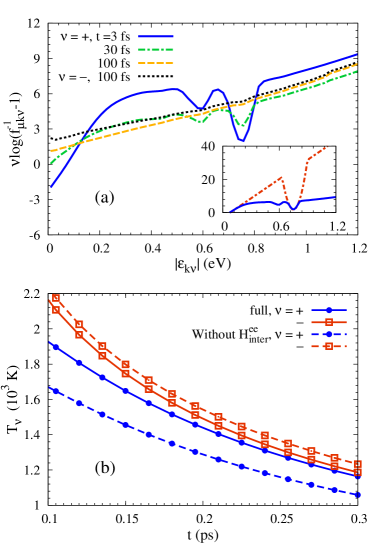
Figure 1: (Color online) (a) $\nu\log(f^{-1}_{\mu{\bf k}\nu}-1)$ as function of $|\varepsilon_{{\bf k}\nu}|$ for conduction-band electrons ($\nu=+$) at $t=3$, 30 and 100 fs and valence band electrons ($\nu=-$) at $t=100$ fs. The results at $t=0$ and $3$ fs for conduction-band electrons are plotted in the inset. (b) Temporal evolution of temperatures of electrons in conduction (blue dots) and valence bands (red squares) from the calculations with (solid curves) and without (dashed curves) the inter-band Coulomb scattering $H^{\rm ee}_{\rm inter}$.

We set the initial carrier distribution to be

$$f_{\mu{\bf k}\nu}=F(\varepsilon_{{\bf k}\nu})+\nu G(\varepsilon_{{\bf k}\nu}),$$ (14)

in which $F(\varepsilon_{{\bf k}\nu})=1/\{1+\exp[(\varepsilon_{{\bf k}\nu}-\mu^{0})/(k_{B}T_{0})]\}$ is the carrier Fermi distribution before pumping with $\mu^{0}$ denoting the initial chemical potential; $G(\varepsilon_{{\bf k}\nu})=A\exp\left[-{(|\varepsilon_{{\bf k}\nu}|-\omega_{\rm pu}/2)^{2}}/(2\Xi^{2})\right]$ is the photo-generated carrier distribution with $A$ and $\Xi$ representing the amplitude and standard deviation, respectively and $\omega_{\rm pu}$ standing for the pump-photon energy. In our computation here, the substrate is chosen to be SiO₂ and the equilibrium carrier density $N_{0}$ is taken to be $6\times 10^{11}$ cm^-2. We also set $A=0.15$, $\Xi=19.3$ meV and $\omega_{\rm pu}=1.5$ eV, corresponding to the excitation density $N_{ex}=8\times 10^{11}$ cm^-2 and the absorbed intensity $I_{a}=1.9$ mJ/m². Then the conduction-band–electron density is about $1.75$ times of the hole density (hole distribution is defined as $f_{\mu{\bf k}h}\equiv 1-f_{\mu{\bf k}-}$). The other parameters are taken to be $T_{0}=300$ K, $E_{\rm max}=0.9$ eV and $\tau_{pp}=3.8$ ps. We first focus on the distribution of the conduction-band electrons and plot the evolution of $\log(f^{-1}_{\mu{\bf k}+}-1)$ in Fig. 1(a). Note that if the distribution $f_{\mu{\bf k}\nu}$ is the Fermi distribution, one has

$$\log(f^{-1}_{\mu{\bf k}\nu}-1)=(\nu v_{\rm F}k-\mu_{\nu})/(k_{B}T_{\nu}),$$ (15)

with $T_{\nu}$ and $\mu_{\nu}$ representing the temperature and chemical potential in the corresponding band. Therefore, if the curves in the figure become linear with $|\varepsilon_{{\bf k}\nu}|$, the buildup of the Fermi distribution is identified. In the inset of Fig. 1(a), one finds a valley located at $|\varepsilon_{{\bf k}\nu}|=0.8$ meV in the initial distribution, coming from the photo-generated carriers. With the evolution of time, the valley is rapidly smeared out by the carrier-carrier Coulomb scattering as shown by the curves with $t=3$ and 30 fs in Fig. 1(a). Moreover, the curve with $t=100$ fs becomes almost linear with $|\varepsilon_{{\bf k}\nu}|$, indicating the buildup of the Fermi distribution. It is noted that this time scale is in the same order as those in the experiments in graphite.Breusing We stress that the hot carrier Fermi distribution presented here is obtained directly from the microscopic kinetic equations and no ansatz is needed as all the scatterings are included.

Then we turn to the valence-band electrons. Our calculations show that the Fermi distribution of the valence-band electrons is established in the same time scale as that of the conduction-band ones, and we only plot $-\log(f^{-1}_{\mu{\bf k}-}-1)$ at $t=100$ fs in Fig. 1(a). More importantly, one finds that the slopes for conduction (black dotted curve) and valence (yellow dashed curve) bands are very close to each other at $t=100$ fs. This indicates that their corresponding temperatures $T_{+}$ and $T_{-}$ are very close to each other [see Eq. (15)], even though the conduction-band–electron density is about $1.75$ times of the hole density. To make this more pronounced, we plot the evolution of the hot-carrier temperatures $T_{\nu}$ fitted from Eq. (15) in Fig. 1(b). The difference between $T_{+}$ and $T_{-}$ is shown to be less than 10%. This phenomenon is due to the strong inter-band Coulomb scattering, which can be seen by comparing the temperatures from the calculations with (solid curves) and without (dashed curves) the inter-band Coulomb scattering $H^{\rm ee}_{\rm inter}$.

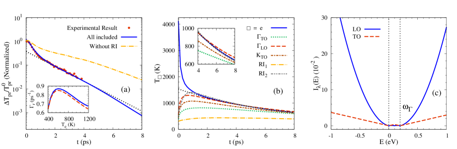
Figure 2: (Color online) (a) DT from the numerical results compared with the experimental results in single-layer graphene on SiO₂ in Ref. Hale, . The calculation without the RI phonons (dash-dotted curve) is also plotted here. The results are normalized as Ref. Hale, . The black dotted curve represents the exponentially fitted curve of the DT in the time range of 2-4 ps. In the inset we plot $\Gamma_{r}$ calculated from Eq. (23) with (solid curve) and without (dashed curve) the second term in the equation. (b) Temporal evolutions of the temperatures of carriers and phonons. Here the carrier temperature is shown to be fitted well by $T_{0}+T_{A}\exp(-\Gamma_{T}t)$ (black dotted curve) for $t>1.5$ ps with $T_{A}=1240$ K and $\Gamma_{T}=0.16$ ps^-1. The inset zooms the time range 4-8 ps. (c) Angular integration $I_{\lambda}(E)$ from Eq. (19) for $\Gamma_{\rm LO}$ and $\Gamma_{\rm TO}$ phonons as function of the carrier energy $E$. The two black dotted lines indicate $E=0$ and $\omega_{\rm\Gamma}$, respectively.

III.2 Temporal evolutions of DT and temperatures of carriers and phonons

As shown in the previous subsection, the hot-carrier Fermi distribution is established very rapidly and the temperatures of electrons in the conduction and valence bands are almost identical. Therefore, in the following calculations, the initial carrier distribution is set to be

$$f_{\mu{\bf k}\nu}(t=0)=1/\{1+\exp[(\varepsilon_{{\bf k}\nu}-\mu^{0}_{\nu})/(k_{B}T^{0}_{e})]\},$$ (16)

where $T^{0}_{e}$ denotes the hot-carrier temperature; $\mu^{0}_{\nu}$ represent the chemical potentials in conduction ($\nu=+$) and valence ($\nu=-$) bands. $T^{0}_{e}$ and $\mu^{0}_{\nu}$ can be determined by the equilibrium carrier density and the excitation density $N_{ex}$ as well as the absorbed intensity $I_{a}$. For simplicity, we set $I_{a}=N_{ex}\omega_{\rm pu}$ with $\omega_{\rm pu}$ denoting the pump-photon energy. With this initial carrier distribution, the evolution of the DT can be obtained numerically.

We first compare the DT from our calculations with the experimental results by Hale et al.Hale in single-layer graphene on SiO₂ substrates [Fig. 2(a)].FitHale Here $T_{0}=300$ K, $\omega_{\rm pr}=1.1$ eV and $\omega_{\rm pu}=1.5$ eV as indicated in the experiment. In this case, the excitation density is much larger than the equilibrium carrier density, thus the chemical potential before the pumping has little influence on the evolution of the DT and is set to be at the Dirac point for simplicity. Then $T^{0}_{e}=4163$ K and $\mu^{0}_{+}=-\mu^{0}_{-}=-478$ meV correspond to $N_{ex}=4.6\times 10^{12}$ cm^-2 and $I_{a}=11$ mJ/m², which are close to the estimated values given in Ref. Hale, . The fitting parameters here are $E_{\rm max}=0.9$ eV and $\tau_{pp}=3.8$ ps. Our results agree very well with the experimental data and show a fast relaxation with the characteristic time about 0.28 ps, followed by a slow one with 1.33 ps.

To reveal the underlying physics of these two relaxations, we plot the evolution of carrier and phonon temperatures in Fig. 2(b). The carrier temperature $T_{e}$ can be obtained by fitting $\log(f^{-1}_{\mu{\bf k}\nu}-1)$. The temperature of hot phonons in $\lambda$ branch can be obtained from $T_{\lambda}=\omega_{\lambda}/[k_{B}\ln(1+1/n_{{\bf q}\lambda})]$. From Fig. 2(b), it is seen that the temperatures of the phonons first increase rapidly and then decrease slowly, with the peaks very close to the crossover point between the fast and slow DT relaxations [see Fig. 2(a)]. Since the fast increase of the phonon temperatures is due to the rapid equilibration of the carrier-phonon system (less than $500$ fs)Breusing ; Kampfrath ; Butscher and the decrease comes from the slow hot-phonon decay (about several picosecond),Yan ; Kang the fast and slow relaxations of the DT can also be attributed to these two processes, respectively.ElecAC This result supports the conjectures in the previous experimental works.Hale ; Wang ; Hwang In addition, by comparing the slow relaxation of the DT with the exponential fitting curve [black dotted curve in Fig. 2(a)], one finds that the relaxation rate slightly increases with the temporal evolution when $t>4$ ps. This can be understood via the approximate formula Eq. (23), which can be rewritten into

$$\Gamma_{r}=\Gamma_{T}\omega_{\rm pr}\frac{T_{e}-T_{0}}{2k_{B}T_{e}^{2}}-\frac{1}{k_{B}T_{e}}\frac{d\mu_{+}}{dt}$$ (17)

by considering that $T_{e}$ can be fitted with $T_{e}=T_{0}+T_{A}\exp^{-\Gamma_{T}t}$ for $t>1.5$ ps, as shown in Fig. 2(b). We plot $\Gamma_{r}$ calculated from this equation with and without the second term in the inset of Fig. 2(a). It is seen that the first term in the equation is dominant and exhibits a peak at $T_{e}=2T_{0}=600$ K. In the time range investigated here, $T_{e}$ is larger than 2$T_{0}$ and thus $\Gamma_{r}$ shows a slight increase with increasing $t$ (decreasing temperature). Nevertheless, in the slow relaxation regime investigated in the experiment, i.e., 2-4 ps, the exponential fit of DT is still acceptable because the corresponding $\Gamma_{r}$ only changes by about 8%.

Figure 2(b) also shows that the temperatures of phonons in different branches are very different, originating from the different carrier-phonon scattering strengths in different phonon branches. Interestingly, the temperatures of the ${\rm\Gamma_{\rm TO}}$ and ${\rm\Gamma_{\rm LO}}$ phonons differ much even though their carrier-phonon scattering matrices are very similar [see Eq. (9)]. This phenomenon comes from their different angular dependences, which is neglected in the simple model in the experimental works.Wang ; Hale To show this more clearly, we utilize the conditions that the carrier distribution is isotropic and the distribution of optical phonons is independent of ${\bf q}$ (i.e., $n_{{\bf q}\lambda}=n_{\lambda}$), and rewrite Eq. (12) as

$$\left.\partial_{t}{n}_{\lambda}\right|_{\rm ep} = \frac{-4\pi}{N_{\rm ph}}\int^{\infty}_{-\infty}dEI_{\lambda}(E)\big{[}f^{<}(E-\omega_{\Gamma})f^{>}(E)n_{\lambda}$$ (18)

$$\mbox{}-f^{>}(E-\omega_{\Gamma})f^{<}(E)(n_{\lambda}+1)\big{]},$$

where $f^{>,<}(E)=\left.f^{>,<}_{\mu{\bf k}\nu}\right|_{\varepsilon_{\mu{\bf k}\nu}=E}$ and the angular integration $I_{\lambda}(E)$ is given by

$$I_{\lambda}(E)=\sum_{{\bf k}\nu\mu\atop{\bf k^{\prime}}\nu^{\prime}\mu^{\prime}}|M^{{\lambda}\mu\mu^{\prime}}_{\bf k\nu,k^{\prime}\nu^{\prime}}|^{2}\delta(\varepsilon_{{\bf k^{\prime}}\nu^{\prime}}-E)\delta(\varepsilon_{{\bf k}\nu}-E+\omega_{\rm\Gamma}).$$ (19)

$I_{\lambda}(E)$ for ${\rm\Gamma_{\rm LO}}$ and ${\rm\Gamma_{\rm TO}}$ phonons are plotted as function of $E$ in Fig. 2(c). One finds that $I_{\lambda}(E)$ for ${\rm\Gamma_{\rm LO}}$ (${\rm\Gamma_{\rm TO}}$) phonons is larger than the other one in the regime $E>\omega_{\rm\Gamma}$ and $E<0$ ($0<E<\omega_{\rm\Gamma}$). For the investigated excitation, $\omega_{\rm pu}$ is much larger than $\omega_{\Gamma}$. Thus the intraband carrier-phonon scattering (corresponding to $E>\omega_{\rm\Gamma}$ and $E<0$) dominates the carrier-phonon thermalization. Consequently, the scattering strength of ${\rm\Gamma_{\rm LO}}$ phonons is stronger and the corresponding temperature is higher. Another more interesting phenomenon shown in Fig. 2(b) is that the carrier temperature can be even lower than the hottest phonon one. This can be understood as follows: When the hot carriers are in equilibrium with the hottest phonons, the cooling of the carrier is due to the energy exchange with the other colder phonons; whereas the cooling of the hottest phonons comes from the anharmonic decay of hot phonons. As shown above, the carrier-phonon thermalization is faster than the hot-phonon decay. Thus the temperature of carrier decreases faster and hence becomes lower than that of the hottest phonons. We also discuss the contribution from the RI phonon, which is neglected in the literatureWang ; Hale by plotting the DT from the calculation without the RI phonons in Fig. 2(a). It is seen that the exclusion of this phonon scattering makes a marked difference, indicating that the RI phonons are very important to the cooling process.

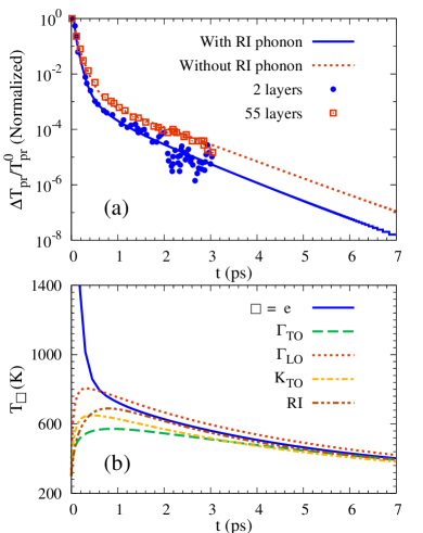
Figure 3: (Color online) (a) Temporal evolution of the DT from the numerical results compared with the experimental data on SiC substrate extracted from Fig. 1 in Ref. Wang, . The results are normalized as that paper. (b) Temporal evolutions of the temperatures of carriers and phonons in the two-layer graphene.

We then investigate the temporal evolutions of DT and temperatures of carriers and phonons in graphene on 6H-SiC. The results are compared with the experimental data reported by Wang et al.Wang (Fig. 1 in that paper) in Fig. 3(a).FitHale As mentioned above, the RI phonons are important only when the number of the graphene layers is small. Therefore, we include the carrier–RI-phonon scattering for the two-layer sample (Sample C in Ref. Wang, ) and exclude it for the 55-layer sample (Sample A). As presented in Ref. Wang, , $\omega_{\rm pu}=\omega_{\rm pr}=1.6$ eV and the average equilibrium carrier densities for 55-layer and two-layer samples are taken to be 1$\times 10^{11}$ cm^-2 and 6$\times 10^{11}$ cm^-2, respectively. $N_{ex}=8.6\times 10^{11}$ cm^-2 and $I_{a}=2$ mJ/m² are consistent with the estimated values in the experiment. Then the corresponding initial temperatures and chemical potentials are $T^{0}_{e}=4193$ K, $\mu^{0}_{+}=-1061$ meV and $\mu^{0}_{-}=1099$ meV for 55-layer sample and $T^{0}_{e}=3512$ K, $\mu^{0}_{+}=-663$ meV and $\mu^{0}_{-}=825$ meV for two-layer sample. The fitting gives $E_{\rm max}=0.8$ eV and $\tau_{pp}=2.5$ ps.

Figure 3(a) shows good agreement between our calculations and the experimental data in both samples, indicating that the contribution from the RI phonons can be responsible for the difference between the DTs in these two cases. It is noted that to fit the results, the carrier–optical-phonon interaction parameters $\langle D^{2}_{\rm\Gamma}\rangle$ and $\langle D^{2}_{\rm K}\rangle$ are chosen to be the same as those adopted in Ref. Wang, but twice of those obtained from the density functional calculations.Piscanec ; Lazzeri In fact, the values of these parameters are still in debate.Piscanec ; Lazzeri ; Rana2 ; Lazzeri2 ; Borysenko Especially, the influences of the electron-electron correlationLazzeri2 ; Attaccalite and the interlayer couplingBorysenko2 on the carrier-phonon interaction parameters in the epitaxial multilayer graphene are still unclear. Thus these parameters can be sample dependent. We also show the evolution of carrier and phonon temperatures in the two-layer graphene in Fig. 3(b). From our results in Fig. 3(a) and (b), it can be seen that the behaviors of carriers and phonons of graphene on a SiC substrate are similar to those on a SiO₂ substrate, i.e., a fast DT relaxation of hundreds of femtoseconds followed by a slower picosecond one as well as a lower carrier temperature compared with the hottest phonons. In addition, the DT in the slow relaxation regime decays exponentially in a large time range. This is because $T_{e}$ is around 2$T_{0}$ where $\Gamma_{r}$ varies mildly with $T_{e}$ as shown in the inset of Fig 2(a).

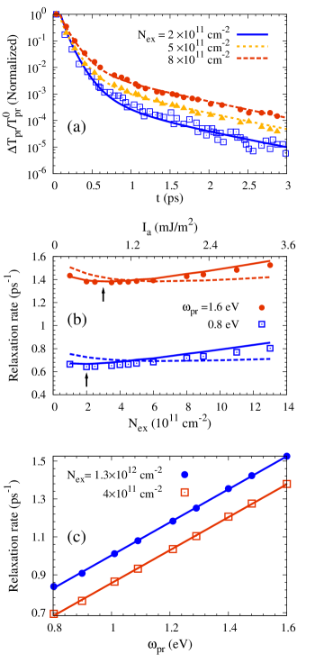
Figure 4: (Color online) (a) DT from the numerical calculations compared with the experimental data [Fig. 3(b) in Ref. Wang, ]. The pump pulse energies in the experiments are 2.5, 6 and 9.8 nJ from the bottom to the top. (b) Slow relaxation rates of the DT from the numerical calculations (dots) and the approximate formula Eq. (23) (solid curves) as function of the excitation density $N_{ex}$ for different probe-photon energies. The DTs calculated from the first term in Eq. (23) (dashed curves) are also plotted here. Note that the scale of $I_{a}$ corresponding to $N_{ex}$ is on top of the frame. The arrows show the positions of the valleys. (c) Slow relaxation rate of the DT as function of the probe-photon energy for different excitation densities. The results are fitted with linear functions (solid lines).

III.3 Excitation-density and probe-photon–energy dependences of the slow DT relaxation

In this subsection, we first compare the calculated DT with the experimental data extracted from Fig. 3(b) in Ref. Wang, for different excitation densities in Fig. 4(a).FitHale Here the parameters are the same as those in Fig. 3 unless otherwise specified and the RI phonons are not included since the layer number of the sample is 16. The fittings give the excitation densities $N_{ex}=2$, 5 and 8$\times 10^{11}$ cm^-2 as well as $E_{\rm max}=0.6$, 0.7 and 0.8 eV for the experimental results with pump-pulse energies being 2.5, 6 and 9.8 nJ, respectively. From this figure, one finds good agreement between our numerical results and the experimental data for all three excitation densities.

By assuming that $E_{\rm max}$ is a linear function of $N_{ex}$ and fitting the above values of $E_{\rm max}$ and $N_{ex}$, we obtain $E_{\rm max}=0.033N_{ex}+0.533$ ($E_{\rm max}$ and $N_{ex}$ are in units of eV and $10^{11}$ cm^-2). With this relation, one can obtain the evolution of DT for other excitation densities. Here we concentrate on the relaxation rate in the time range of 2-3 ps, since the evolution of DT in this regime shows a good exponential decay in the whole excitation density range in this investigation. The results are plotted as dots in Fig. 4(b). It is seen that mild valleys appear in the $N_{ex}$ dependence and the excitation densities where valleys appear tend to be lower for smaller $\omega_{\rm pr}$. To better understand this phenomenon, we also plot the results from the approximate formula Eq. (23) (solid curves) in Fig. 4(b). Here $T_{e}$, $dT_{e}/dt$ and $d\mu_{+}/dt$ in Eq. (23) are chosen to be the ones at the middle of this time region, i.e., $t=2.5$ ps for each $N_{ex}$. One can see that the results from Eq. (23) agree very well with those from the kinetic equations and exhibit valleys at the same $N_{ex}$. The scenario of these valleys is as follows. With the increase of excitation density, the carrier and phonon temperatures increase. Thus the electron-hole recombination and the cooling of carrier-phonon system both accelerate due to the enhanced carrier-phonon and phonon-phonon scatterings. As a result, $-d\mu_{+}/dt$ and $-dT_{e}/dt$ in Eq. (23) increase with $N_{ex}$. Furthermore, our calculations show that $-d\mu_{+}/dt$ almost increases linearly with $N_{ex}$ and $-dT_{e}/dt\sim N^{0.3}_{ex}$ in the excitation density range investigated here. The excitation-density dependence of $T_{e}$ is more complex: for $T_{e}\sim N^{\alpha}_{ex}$, $\alpha$ is around 0.18 for $1\times 10^{11}$ cm${}^{-2}<N_{ex}<5\times 10^{11}$ cm^-2 and then decreases slowly with increasing $N_{ex}$ and reaches $0.1$ for $N_{ex}=1.3\times 10^{12}$ cm^-2. Therefore, the first term in Eq. (23) first decreases and then increases with increasing $N_{ex}$, while the second term increases monotonically with $N_{ex}$. Under the joint effects of these two terms, the relaxation rate shows a valley at the excitation density lower than that solely from the first term [dashed curves in Fig. 4(b)]. Also by considering that the contribution of the first term decreases with decreasing $\omega_{\rm pr}$, the valley moves to lower $N_{ex}$ when $\omega_{\rm pr}$ becomes smaller. We also present more detail about the probe-photon–energy dependence in Fig. 4(c). It is seen that the relaxation rate increases linearly with the increase of probe-photon energy $\omega_{\rm pr}$. This can also be understood via Eq. (23) if one notices that $\mu_{+}$ and $T_{e}$ are independent of $\omega_{\rm pr}$.

IV CONCLUSION

In conclusion, we have microscopically investigated the dynamics of nonequilibrium carriers and phonons in graphene by solving the kinetic equations with the carrier-phonon and the carrier-carrier scatterings explicitly included. The hot-carrier Fermi distribution is found to be established within 100 fs. Furthermore, the temperatures of electrons in conduction and valence bands are shown to be very close to each other even when the excitation density is comparable with the equilibrium carrier density. This is shown to be due to the strong inter-band Coulomb scattering. Moreover, the temporal evolutions of the DT obtained from the kinetic equations agree well with the experimental resultsHale ; Wang for different graphene layer numbers and excitation densities, with a fast relaxation about hundreds femtoseconds followed by a slow picosecond one presented. Based on the results of the evolutions of carrier and phonon temperatures, we find that the mechanisms leading to these two relaxations are the fast carrier-phonon thermalization and the hot-phonon decay, respectively, which is consistent with the conjecture in the previous experimental works.Wang ; Hale ; Huang We also show that the temperatures of the hot phonons in various branches are very different due to their different carrier-phonon scattering strengths. Particularly, in spite of the similar carrier-phonon interaction matrices, the scattering strengths of the TO and LO phonons near the $\Gamma$ point are very different due to their different angular dependences. In addition, the temperature of carriers can be lower than that of the hottest phonons. This comes from the fact that the phonon temperatures are different for different branches and the hot-phonon decay is unimportant during the phonon thermalization. Our calculations also show that the contribution of the RI phonons is important in the relaxation process.

Finally, we investigate the excitation-density and the probe-photon–energy dependences of the slow DT relaxation rate. The relaxation rate is found to exhibit a mild valley in the excitation density dependence. This phenomenon comes from the competition among the increasing carrier temperature and the accelerating electron-hole recombination and carrier-phonon cooling with an increase of the excitation density. We also show that the slow relaxation rate is linear with the probe-photon energy.

*

Appendix A Approximate formula of slow relaxation rate of DT

We present the derivation of the approximate formula of the slow relaxation rate of DT here. In this time region, the Fermi distribution has been established. Thus the distribution functions for electrons in the conduction and valence bands are $f_{c}=\{\exp[\beta(\omega_{\rm pr}/2-\mu_{+})]+1\}^{-1}$ and $f_{v}=\{\exp[\beta(-\omega_{\rm pr}/2-\mu_{-})]+1\}^{-1}$, with $\beta=1/(k_{B}T_{e})$. Since $N_{\rm lay}\sigma(\omega_{\rm pr})\sqrt{\mu_{0}/\epsilon_{0}}/(1+n_{\rm ref})\ll 1$,

$$T_{\rm pr} \approx 1+\frac{N_{\rm lay}e^{2}\sqrt{{\mu_{0}}/{\epsilon_{0}}}}{2(1+n_{\rm ref})}\left[\frac{1}{e^{\beta(\omega_{\rm pr}/2-\mu_{+})}+1}\right.$$ (20)

$$\mbox{}-\left.\frac{1}{e^{\beta(-\omega_{\rm pr}/2-\mu_{-})}+1}\right].$$

Also considering that $\omega_{\rm pr}$ is much larger than $\mu_{+}$, $\mu_{-}$ and $k_{B}T_{e}$, $\Delta T_{\rm pr}\equiv T_{\rm pr}-T^{0}_{\rm pr}$ can be expressed as

$$\Delta T_{\rm pr}\approx\frac{e^{2}N_{\rm lay}\sqrt{\mu_{0}/\epsilon_{0}}}{2(1+n_{\rm ref})}e^{-\beta\omega_{\rm pr}/2}(e^{\beta\mu_{+}}+e^{-\beta\mu_{-}}).$$ (21)

Thus, the relaxation rate of DT is given by

$$\Gamma_{r} \equiv -\frac{1}{\Delta T_{\rm pr}}\frac{d}{dt}(\Delta T_{\rm pr})$$ (22)

$$\approx \frac{\omega_{\rm pr}}{2}\frac{d\beta}{dt}-\beta\frac{d\mu_{+}}{dt}+\beta\frac{(\frac{d\mu_{+}}{dt}+\frac{d\mu_{-}}{dt})}{e^{\beta(\mu_{+}+\mu_{-})}+1}.$$

In the excitation density range investigated here, $|d\mu_{+}/dt+d\mu_{-}/dt|\ll|d\mu_{+}/dt|$. Therefore, one has

$$\Gamma_{r}=-\frac{\omega_{\rm pr}}{2k_{B}T^{2}_{e}}\frac{dT_{e}}{dt}-\frac{1}{k_{B}T_{e}}\frac{d\mu_{+}}{dt}.$$ (23)

References

- (1) K. S. Novoselov, A. K. Geim, S. V. Morozov, D. Jiang, Y. Zhang, S. V. Dubonos, I. V. Grigorieva, and A. A. Firsov, Science 306, 666 (2004).
- (2) K. S. Novoselov, A. K. Geim, S. V. Morozov, D. Jiang, M. I. Katsnelson, I. V. Grigorieva, S. V. Dubonos, and A. A. Firsov, Nature 438, 197 (2005).
- (3) A. H. Castro Neto, F. Guinea, N. M. R. Peres, K. S. Novoselov, and A. K. Geim, Rev. Mod. Phys. 81, 109 (2009).
- (4) F. Schedin, A. K. Geim, S. V. Morozov, E. W. Hill, P. Blake, M. I. Katsnelson, and K. S. Novoselov, Nat. Mater. 6, 652 (2007).
- (5) F. Wang, Y. Zhang, C. Tian, C. Girit, A. Zettl, M. Crommie, and Y. Ron Shen, Science 320, 206 (2008).
- (6) J. M. Dawlaty, S. Shivaraman, M. Chandrashekhar, F. Rana, and M. G. Spencer, Appl. Phys. Lett. 92, 042116 (2008).
- (7) P. J. Hale, S. M. Hornett, J. Moger, D. W. Horsell, and E. Hendry, Phys. Rev. B 83, 121404(R) (2011).
- (8) H. Wang, J. H. Strait, P. A. George, S. Shivaraman, V. B. Shields, M. Chandrashekhar, J. Hwang, F. Rana, M. G. Spencer, C. S. Ruiz-Varges, and J. Park, Appl. Phys. Lett. 96, 081917 (2010).
- (9) L. Huang, G. V. Hartland, L. Chu, Luxmi, R. M. Feenstra, C. Lian, K. Tahy, and H. Xing, Nano Lett. 10, 1308 (2010).
- (10) M. Breusing, C. Ropers, and T. Elsaesser, Phys. Rev. Lett. 102, 086809 (2009).
- (11) T. Kampfrath, L. Perfetti, F. Schapper, C. Frischkorn, and M. Wolf, Phys. Rev. Lett. 95, 187403 (2005).
- (12) S. Butscher, F. Milde, M. Hirtschulz, E. Malić, and A. Knorr, Appl. Phys. Lett. 91, 203103 (2007).
- (13) H. Yan, D. Song, K. F. Mak, I. Chatzakis, J. Maultzsch, and T. F. Heinz, Phys. Rev. B 80, 121403(R) (2009).
- (14) K. Kang, D. Abdula, D. G. Cahill, and M. Shim, Phys. Rev. B 81, 165405 (2010).
- (15) S. Piscanec, M. Lazzeri, F. Mauri, A. C. Ferrari, and J. Robertson, Phys. Rev. Lett. 93, 185503 (2004).
- (16) M. Lazzeri, S. Piscanec, F. Mauri, A. C. Ferrari, and J. Robertson, Phys. Rev. Lett. 95, 236802 (2005).
- (17) T. Ando, J. Phys. Soc. Jpn. 75, 124701 (2006).
- (18) M. W. Wu, J. H. Jiang, and M. Q. Weng, Phys. Rep. 493, 61 (2010); and references therein.
- (19) Y. Zhou and M. W. Wu, Phys. Rev. B 82, 085304 (2010).
- (20) P. Zhang and M. W. Wu, Phys. Rev. B 84, 045304 (2011).
- (21) P. Zhang and M. W. Wu, arXiv:1108.0283.
- (22) H. Haug and A.-P. Jauho, Quantum Kinetics in Transport and Optics of Semiconductors (Springer, Berlin, 1998).
- (23) E. H. Hwang, S. Adam, and S. Das Sarma, Phys. Rev. Lett. 98, 186806 (2007).
- (24) E. H. Hwang and S. Das Sarma, Phys. Rev. B 75, 205418 (2007).
- (25) S. Adam, E. H. Hwang, V. M. Galitski, and S. Das Sarma, Proc. Natl. Acad. Sci. U.S.A. 104, 18392 (2007).
- (26) S. Adam and S. Das Sarma, Solid State Commun. 146, 356 (2008).
- (27) S. Fratini and F. Guinea, Phys. Rev. B 77, 195415 (2008).
- (28) B. Wunsch, T. Stauber, F. Sols, and F. Guinea, New J. Phys. 8, 318 (2006).
- (29) X.-F. Wang and T. Chakraborty, Phys. Rev. B 75, 033408 (2007).
- (30) M. R. Ramezanali, M. M. Vazifeh, R. Asgari, M. Polini, and A. H. MacDonald, J. Phys. A: Math. Theor. 42, 214015 (2009).
- (31) E. H. Hwang and S. Das Sarma, Phys. Rev. B 77, 115449 (2008).
- (32) J.-H. Chen, C. Jang, S. Xiao, M. Ishigami, and M. S. Fuhrer, Nat. Nanotechnol. 3, 206 (2008).
- (33) V. Perebeinos and P. Avouris, Phys. Rev. B 81, 195442 (2010).
- (34) Unlike Refs. Hale, and Wang, , we do not set the minimum value of participating in the carrier-phonon scattering to be , since the phonons with can be heated by the inter-band carrier-phonon scattering.
- (35) M. Q. Weng, M. W. Wu, and L. Jiang, Phys. Rev. B 69, 245320 (2004).
- (36) V. P. Gusynin, S. G. Sharapov, and J. P. Carbotte, Phys. Rev. Lett. 96, 256802 (2006).
- (37) N. M. R. Peres, F. Guinea, and A. H. Castro Neto, Phys. Rev. B 73, 125411 (2006).
- (38) F. Rana, IEEE Trans. Nanotechnol. 7, 91 (2008).
- (39) J. M. Dawlaty, S. Shivaraman, J. Strait, P. George, M. Chandrashekhar, F. Rana, M. G. Spencer, D. Veksler, and Y. Chen, Appl. Phys. Lett. 93, 131905 (2008).
- (40) S. Latil, V. Meunier, and L. Henrard, Phys. Rev. B 76, 201402(R) (2007).
- (41) F. Varchon, P. Mallet, L. Magaud, and J.-Y. Veuillen, Phys. Rev. B 77, 165415 (2008).
- (42) G. Ghosh, Opt. Commun. 163, 95 (1999).
- (43) D. S. Novikov, Phys. Rev. B 76, 245435 (2007).
- (44) M. E. Levinshtein, S. L. Rumyantsev, and M. S. Shur, Properties of Advanced Semiconductor Materials: GaN, AlN, InN, BN, SiC, SiGe (John Wiley & Sons, New York, 2001).
- (45) Since the pumping process is not simulated in this investigation, we shift the experimental results in Figs. 2(a), 3(a) and 4(a) by , and fs, respectively.
- (46) Our calculations show that the electron-acoustic-phonon scattering is negligible for the evolution of the DT (not shown in the figure).
- (47) M. Lazzeri, C. Attaccalite, L. Wirtz, and F. Mauri, Phys. Rev. B 78, 081406(R) (2008).
- (48) F. Rana, P. A. George, J. H. Strait, J. Dawlaty, S. Shivaraman, M. Chandrashekhar, and M. G. Spencer, Phys. Rev. B 79, 115447 (2009).
- (49) K. M. Borysenko, J. T. Mullen, E. A. Barry, S. Paul, Y. G. Semenov, J. M. Zavada, M. Buongiorno Nardelli, and K. W. Kim, Phys. Rev. B 81, 121412(R) (2010).
- (50) C. Attaccalite, L. Wirtz, M. Lazzeri, F. Mauri, and A. Rubio, Nano Lett. 10, 1172 (2010).
- (51) K. M. Borysenko, J. T. Mullen, X. Li, Y. G. Semenov, J. M. Zavada, M. Buongiorno Nardelli, and K. W. Kim, Phys. Rev. B 83, 161402(R) (2011).