Dynamical mean-field theories of correlation and disorder

Chapter 0 Dynamical mean-field theories of correlation and disorder

1 Mott transitions in clean and disordered systems

It is this fascination with the local and with the failures, not successes, of band theory, which…  contradicted the assumptions of the time…
P. W. Anderson, Nobel Prize Lecture, 1979

1 Introduction

The Dynamical Mean Field Theory (DMFT) of interacting lattice fermions is perhaps best described as the optimal description of these systems which takes into account only local (on-site) correlation effects Pruschke1995,georgesrmp. Technically, this is implemented through the assumption of a single-electron self-energy which, in the lattice translationally invariant case, is independent of the site in real space or of wave vector in reciprocal space and therefore is a function of frequency only

$$\Sigma\left(\boldsymbol{R_{i}},\omega\right)\to\Sigma\left(\omega\right)\qquad\mathrm{or}\qquad\Sigma\left(\boldsymbol{k},\omega\right)\to\Sigma\left(\omega\right).$$

This kind of approximation surely leaves out inter-site correlations. However, local approaches to strong correlations have a long history and several semi-phenomenological descriptions of classes of compounds within this framework have been shown to be consistent with their physical properties. A particularly well-studied example are heavy fermion systems Stewart1984,Grewe1991. Many properties of heavy fermion materials suggest that local correlations are sufficient for a good description, the large carrier effective mass (as derived from the magnetic susceptibility or the Sommerfeld specific heat linear coefficient) being the best known but by no means the only ones. Transport properties such as DC and optical conductivity and ultrasound attenuation can also be understood with the same assumptions varma85. Other examples of systems well described by a local approach include systems close to a Mott metal-insulator transition, in particular, the vicinity of the finite-temperature critical end-point Rozenberg1999a,Kotliar2000,Kotliar2002,Limelette03,Limelette2003,kagawaetal05. A particularly striking consequence of a local self-energy is the cancellation of many-body renormalizations in the ratio of the coefficient of the $T^{2}$-term of the resistivity to the square of the specific heat coefficient, usually called the Kadowaki-Woods ratio KadowakiWoods,Miyakeetal89. Recently, it has been shown that, when materials-specific effects (such as carrier density, density of states and Fermi velocity values) are properly taken into account, then the Kadowaki-Woods ratio appears to be universal across a much wider range of compounds, including, besides heavy fermion systems, organic charge-transfer salts, transition-metal oxides, and transition metals jackoetal09. Thus, a local approach to strong correlations seems to be much more generally valid than initially thought.

Several starting points lead to theories that ultimately predict a self-energy of this form, most notably descriptions based on the Gutzwiller wave-function Gutzwiller1963,Gutzwiller1965,Vollhardt1984 or the large-N limit colemanlong,millislee87. However, these theories usually end up imposing further restrictions, beyond a local self-energy, e. g., inelastic scattering effects are not included, higher-energy incoherent features are absent, among others. A description which incorporates all possible local effects in a fully self-consistent fashion is provided by DMFT.

Historically, DMFT was proposed by a recourse to the infinite-dimensional limit of lattice systems MetznerVollhardt89. Indeed, when appropriate rescaling of parameters is done (as is usual when considering this limit), the theory remains meaningful and non-trivial as $d\to\infty$ and the self-energy becomes completely local. The reader can find many alternative derivations of DMFT in this limit in the review georgesrmp. Alternatively, DMFT can also be viewed as the best local description of three-dimensional systems. The focus here will not be to derive the theory by resorting to the infinite-dimensional limit but rather to highlight the physical content of a local description of correlation effects. This is specially important since we will later explore other, more general local theories which do not become exact in any particular limit but which inherit the insights gained from DMFT. We will therefore focus mostly on a Bethe lattice, which is most transparent and lends itself particularly well to generalizations to the disordered case. Furthermore, we will highlight the key physical assumptions involved, which are kept in the other approximations.

2 The clean case

Consider for concreteness the Hubbard model with only nearest-neighbor hopping on a lattice with finite coordination $z$, in usual notation,

$$H = -\sum_{\left\langle ij\right\rangle,\sigma}t_{ij}c_{i\sigma}^{\dagger}c_{j\sigma}+U\sum_{i}n_{i\uparrow}n_{i\downarrow}.$$ (1)

We focus on a particular site, call it $j$, which in the clean case can be any site. The effective dynamics of this site alone can be obtained by integrating out all the other sites. This is no longer a Hamiltonian dynamics and the procedure requires an action description, which we will write in imaginary time

$$S_{eff}\left(j\right) = \sum_{\sigma}\int_{0}^{\beta}d\tau c_{j\sigma}^{\dagger}\left(\tau\right)\left(\partial_{\tau}-\mu\right)c_{j\sigma}\left(\tau\right)$$ (2)

$$+ \sum_{\sigma}\int_{0}^{\beta}d\tau\int_{0}^{\beta}d\tau^{\prime}c_{j\sigma}^{\dagger}\left(\tau\right)\Delta\left(\tau-\tau^{\prime}\right)c_{j\sigma}\left(\tau^{\prime}\right)$$

$$+ U\int_{0}^{\beta}d\tau n_{j\uparrow}\left(\tau\right)n_{j\downarrow}\left(\tau\right).$$

The second term above comes from integrating out the other sites, the first and third ones being the local contributions, already present before the integration. The thing to note here is the fact that, in general, the integration over interacting sites generates other higher-order terms, involving four and more fermionic fields. In the high-dimensional limit or in DMFT in general, these higher-order terms are absent or neglected. It is clear that this means that only single-particle inter-site correlations are kept in this limit/approximation and this is precisely what is encoded in the second, retarded term in Eq. (2). The “hybridization function” $\Delta\left(\tau\right)$ describes the “leaking” of electrons in and out of site $j$. It can be written as

$$\Delta\left(\tau\right)=t^{2}\sum_{l,m=1}^{z}G_{lm}^{\left(j\right)}\left(\tau\right),$$ (3)

where $G_{lm}^{\left(j\right)}\left(\tau\right)$ is the Green’s function for propagation from site $m$ to site $l$ in a lattice from which site $j$ has been removed (hence the superscript $\left(j\right)$)

$$G_{lm}^{\left(j\right)}\left(\tau\right)=-\left\langle T\left[c_{l\sigma}\left(\tau\right)c_{m\sigma}^{\dagger}\left(0\right)\right]\right\rangle^{\left(j\right)},$$ (4)

and the sums extend over the $z$ nearest-neighbors of site $j$. Let us not dwell on how this is calculated for now.

The action (2) is equivalent to the one of an Anderson single-impurity problem Anderson1961, whose Hamiltonian is

$$H = \sum_{\boldsymbol{k},\sigma}E_{\boldsymbol{k}}a_{\boldsymbol{k}\sigma}^{\dagger}a_{\boldsymbol{k}\sigma}-\sum_{\sigma}\mu c_{j\sigma}^{\dagger}c_{j\sigma}$$ (5)

$$+ \sum_{\boldsymbol{k},\sigma}\left(\frac{V_{\boldsymbol{k}}}{\sqrt{N_{s}}}a_{\boldsymbol{k}\sigma}^{\dagger}c_{j\sigma}+\mathrm{H.c.}\right)+Uc_{j\uparrow}^{\dagger}c_{j\uparrow}c_{j\downarrow}^{\dagger}c_{j\downarrow},$$

provided we choose $E_{\boldsymbol{k}}$ and $V_{\boldsymbol{k}}$ above in such a way that the Fourier transform, in Matsubara frequency space, of the hybridization function in Eq. (3) is such that

$$\Delta\left(i\omega_{n}\right)=\frac{1}{N_{s}}\sum_{\boldsymbol{k}}\frac{\left|V_{\boldsymbol{k}}\right|^{2}}{i\omega_{n}-E_{\boldsymbol{k}}}.$$ (6)

This equivalence proves to be extremely useful since the well-studied behavior of the Anderson single-impurity problem serves as a guide to physical insight georgeskotliar92.

Suppose now that we can somehow find the full interacting Green’s function of the system described by the action of Eq. (2)

$$G_{jj}\left(\tau\right)=-\left\langle T\left[c_{j\sigma}\left(\tau\right)c_{j\sigma}^{\dagger}\left(0\right)\right]\right\rangle_{eff},$$ (7)

where the subscript $eff$ emphasizes that it is to be calculated under the dynamics dictated by (2). We can repackage our ignorance about this function by defining a self-energy $\Sigma\left(i\omega_{n}\right)$ such that

$$G_{jj}\left(i\omega_{n}\right)=\frac{1}{i\omega_{n}+\mu-\Delta\left(i\omega_{n}\right)-\Sigma\left(i\omega_{n}\right)}.$$ (8)

Having quantified the local dynamics, we now need to bring in information from the rest of the lattice. In principle, this is quite straightforward: since only local correlations are included, $\Sigma\left(i\omega_{n}\right)$ is also the self-energy for generic lattice propagation

$$G\left(\boldsymbol{k},i\omega_{n}\right)=\frac{1}{i\omega_{n}-\varepsilon_{\boldsymbol{k}}+\mu-\Sigma\left(i\omega_{n}\right)},$$ (9)

where $\varepsilon_{\boldsymbol{k}}$ is the non-interacting dispersion. From this expression, we can obtain the Green’s function with one site removed from Eq. (4) and from that the hybridization function (3), which closes the self-consistency loop. This procedure to get $\Delta\left(i\omega_{n}\right)$ from $G\left(\boldsymbol{k},i\omega_{n}\right)$ is described, e. g., in the review georgesrmp. However, we will proceed in the simpler and more illuminating case of the Bethe lattice with coordination $z$, for which

$$G_{lm}^{\left(j\right)}\left(\tau\right)=\delta_{lm}G_{ll}^{\left(j\right)},$$ (10)

since the removal of site $j$ completely disconnects the two branches that start at the nearest-neighbors $l$ and $m$, if $l\neq m$. Thus,

$$\Delta\left(\tau\right) = t^{2}\sum_{l=1}^{z}G_{ll}^{\left(j\right)}\left(\tau\right)$$ (11)

$$= zt^{2}G_{ll}^{\left(j\right)}\left(\tau\right),$$ (12)

since all sites are equivalent. We can now take the limit $z\to\infty$, noting that, in this limit, the removal of one nearest-neighbor site ($j$) is irrelevant for the local propagation at $l$ and that an appropriate rescaling, namely $zt^{2}\to\tilde{t}^{2}$, is necessary

$$\Delta\left(\tau\right)=\tilde{t}^{2}G_{ll}\left(\tau\right)=\tilde{t}^{2}G_{jj}\left(\tau\right),$$ (13)

since all sites are equivalent. This is the self-consistency condition in this case: the solution of the problem is the one for which, if we plug in the local Green’s function $G_{jj}\left(\tau\right)$ in Eq. (13), then insert it into the action (2) and find the expectation value in Eq. (7), we get back $G_{jj}\left(\tau\right)$.

A more physical alternative route and one which is not restricted to the Bethe lattice is to note that the local Green’s function obtained from (9) must coincide with the one defined in (8)

$$G_{jj}\left(i\omega_{n}\right) = \frac{1}{N_{s}}\sum_{\boldsymbol{k}}G\left(\boldsymbol{k},i\omega_{n}\right)\Rightarrow$$

$$\frac{1}{i\omega_{n}+\mu-\Delta\left(i\omega_{n}\right)-\Sigma\left(i\omega_{n}\right)} = \int d\varepsilon\frac{\rho_{0}\left(\varepsilon\right)}{i\omega_{n}-\varepsilon+\mu-\Sigma\left(i\omega_{n}\right)}.$$ (14)

Here, $\rho_{0}\left(\varepsilon\right)$ is the bare density of states generated from $\varepsilon_{\boldsymbol{k}}$. The two procedures can be shown to be equivalent and establish the necessary self-consistency condition.

It is possible to extend the above analysis to two-particle correlation functions georgesrmp but we will not delve into it. It is, however, worthwhile to notice that the current-current correlation function, which provides the conductivity through the Kubo formula acquires no vertex correction within DMFT and is given by a simple bubble of renormalized single-particle Green’s functions.

It is perhaps wise to highlight yet again what the key assumptions of this approach are:

1. The effects of interactions that are included are on-site only, or equivalently, the self-energy is purely local.

2. Different sites “know” about each other through single-particle processes only, see Fig. 1(a).

3. The local dynamics, as dictated by the local effective action and usually encoded in the local Green’s function, must coincide with the local dynamics as derived from the lattice propagation.

The DMFT approach, like the original Bragg-Williams (BW) mean-field theory of magnetism goldenfeldbook, focuses on a single lattice site, but replaces its environment by a self-consistently determined “effective medium” georgesrmp. Unlike the BW theory, the effect of the environment cannot be captured by a static external field, but must be encoded in a full complex function $\Delta\left(i\omega_{n}\right)$, which contains information about the dynamics of an electron moving in and out of the given site. The calculation then reduces to solving an appropriate quantum impurity problem, Eq. (2), supplemented by an additional self-consistency condition, Eq. (14), that ultimately determines this hybridization function $\Delta(i\omega_{n})$.

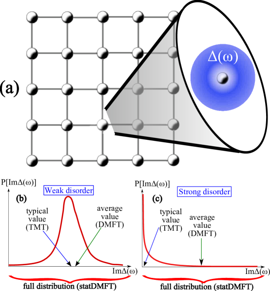
Figure 1: Schematic view of all DMFT-inspired theories of disordered strongly correlated systems. (a) All these theories share the same ingredient: the local site “knows” about the other sites through the self-consistently determined hybridization function $\Delta\left(\omega\right)$ (see Eq. (2)), which acts as an order parameter. They differ in the level of description of this order parameter, which is in general a random quantity (panels b and c). Both DMFT and the Typical Medium Theory (TMT) replace the actual local realization of this random variable by a fixed, non-random function, namely, the average and the typical values of $\Delta\left(\omega\right)$, respectively. These two functions are very similar at weak disorder (panel b), but become increasingly different as the disorder grows (panel c). The statistical dynamical mean field theory (statDMFT), by contrast, retains the full spectrum of spatial fluctuations, since each site “sees” the actual local realization $\Delta_{i}\left(\omega\right)$.

The approach has been very successful in examining the vicinity of the Mott transition in clean systems, in which it has met spectacular success in elucidating various properties of several transition metal oxides georgesrmp, heavy fermion systems, and even Kondo insulators re:Rozenberg96.

3 The clean Mott transition

The Mott transition in a single-band Hubbard model can be regarded as a prototype for a interaction-driven metal-insulator transition, a phenomenon with plausible relevance to many physical systems of current interest. Its basic mechanism has been correctly understood for more than fifty years mott1949, yet the precise nature of this phase transition has long remained controversial and ill-understood. Part of the confusion stems from the fact that at low temperatures the Mott insulator is typically unstable to antiferromagnetic ordering, leading many authors slater51 to focus on magnetism as a proposed driving force. The shortcoming of this view was most lucidly emphasized by Anderson andersonlocrev who stressed that the Mott insulating state persists well above the Néel temperature. It is thus transmutation of conduction electrons into local magnetic moments - not the long range magnetic ordering - that should be regarded as the fundamental physical process behind the Mott transition. The two phenomena can be most clearly separated in systems where the tendency for magnetic ordering can be appreciably weakened due to frustration effects, such as often found in orbitally degenerate transition metal oxides. Here, the competition between antiferromagnetic superexchange and ferromagnetic tendencies due to Hund’s rule couplings typically lead to large cancellations, resulting in very weak magnetic correlations in the paramagnetic phase.

From the theoretical point of view, this situation can be most clearly formulated by focusing on the “maximally frustrated” Hubbard model, with infinite-range hopping of random sign georgesrmp. In this model the magnetic frustration is so strong as to completely suppress any magnetic ordering, while the DMFT approximation becomes exact, allowing precise and detailed characterization of such an “ideal” Mott transition within the paramagnetic phase. In the following we briefly describe the main features of the resulting DMFT picture of the bandwidth-driven Mott transition.

Critical behavior and mass divergence at $T=0$

Within DMFT, the critical regime between the Fermi liquid metal and the Mott insulator features georgesrmp a finite temperature coexistence region and a first-order transition line ending at the critical end-point at $T=T_{c}$. At $T=0$, however, the metallic solution is the stable (lower energy) one throughout the coexistence regime. It is characterized by heavy quasiparticles (QP) with an effective mass that diverges as the transition is approached.

In general, the effective mass is evaluated from the single-particle self-energy using the expression

$${\frac{m^{\ast}}{m}}=\left.{\frac{1-{\frac{\partial}{\partial\omega}}\Sigma^{\prime}(\mathbf{k},\omega)}{1+{\frac{m}{k}}{\frac{\partial}{\partial k}}\Sigma^{\prime}(\mathbf{k},\omega)}}\right|_{k=k_{F},\omega=0},$$ (15)

where $k_{F}$ denotes the Fermi momentum, and $\Sigma^{\prime}$ is the real part of the self-energy $\Sigma(\mathbf{k},\omega)$. The QP weight, on the other hand, is defined by

$$Z^{-1}\equiv\left.1-{\frac{\partial}{\partial\omega}}\Sigma^{\prime}(\mathbf{k},\omega)\right|_{k=k_{F},\omega=0}.$$ (16)

Within DMFT, $\Sigma(\mathbf{k},\omega)=\Sigma(\omega)$ is momentum independent, and $m^{\ast}/m=Z^{-1}$. Note that, since generally $\left.{\frac{\partial}{\partial\omega}}\Sigma^{\prime}(\omega)\right|_{\omega=0}<0$, the interactions increase the effective mass. The actual divergence is obtained only if the quantity $A\equiv\left.-{\frac{\partial}{\partial\omega}}\Sigma^{\prime}(\omega)\right|_{\omega=0}$ itself diverges. This scenario is realized, for example, in the Brinkmann-Rice theory of the Mott transition, as well as in the more recent DMFT solution. Since the QP weight is simply $Z^{-1}=m^{\ast}/m$, it must diverge at the same place as $m^{\ast}$ does.

We should emphasize that this result is exact within the DMFT approach and is an excellent approximation for many Mott compounds where magnetic frustration is sufficiently strong. To put this result in perspective, we contrast it with a popular but uncontrolled weak-coupling approach, based on the so-called “on-shell approximation” quinn75prl for the effective mass of the correlated electron gas. Here, an approximate expression for the effective mass is proposed

$${\frac{m^{\ast}}{m}}\approx\left.{\frac{1}{1+{\frac{m}{k}}{\frac{d}{dk}}\Sigma^{\prime}(\mathbf{k},\xi_{\mathbf{k}})}}\right|_{k=k_{F}},$$ (17)

where $\xi_{\mathbf{k}}$ is the unrenormalized band dispersion. When this approximation is applied to the low-density electron gas within the Random Phase Approximation (RPA) scheme dassarma05prb, one finds that the effective mass diverges before the QP weight $Z$ vanishes. This result seems quite pathological, since the natural interpretation of the effective mass divergence is the localization of itinerant electrons, where one also expects the breakdown of the quasiparticle picture.

To benchmark the validity of the proposed “on-shell approximation”, we apply it to the maximally frustrated Hubbard model, where DMFT provides us with an exact result for both the effective mass and the full self-energy. In this case $\Sigma^{\prime}(\mathbf{k},\omega=\xi_{\mathbf{k}})=\Sigma^{\prime}(\omega\mathbf{=}\xi_{\mathbf{k}})$. Noting that

$$\left.{\frac{m}{k}}{\frac{d}{dk}}\Sigma^{\prime}(\omega=\xi_{\mathbf{k}})\right|_{k=k_{F}}=\left.{\frac{\partial}{\partial\omega}}\Sigma^{\prime}(\omega)\right|_{\omega=0},$$

we get the “on-shell” result

$${\frac{m^{\ast}}{m}}\approx\left.{\frac{1}{1+{\frac{\partial}{\partial\omega}}\Sigma^{\prime}(\omega)}}\right|_{\omega=0}={\frac{1}{1-A}}.$$

As we can see, this expression is equivalent to the exact expression $m^{\ast}/m=1+A$, only to leading order, i.e. for $(1-Z)\ll 1$. On the other hand, the positive quantity $A$ is expected to grow with the interaction. As long as it is finite, neither will the properly defined effective mass $m^{\ast}/m,$ nor the inverse QP weight $Z^{-1}$ ever diverge. In contrast, if one uses the “on-shell” expression, then the effective mass will blow up as soon as $A=1$, and this will happen at some point in any approximation where $A$ grows with the interaction. However, as we can see, this will not lead to the divergence of the inverse QP weight $Z^{-1}$. What we can see from these expressions is that the essence of the “on-shell” approximation is simply to linearize the expression for $(m^{\ast}/m)^{-1}$, by expanding it in the quantity $A\equiv\left.-{\frac{\partial}{\partial\omega}}\Sigma^{\prime}(\omega)\right|_{\omega=0}.$ Instead of appearing in the numerator of the effective mass expression, it now enters the denominator, leading to an unphysical effective mass divergence. This example provides a perfect illustration of how dangerous it is to indiscriminately apply weak-coupling results to non-perturbative phenomena near the Mott transition. It also shows how DMFT not only correctly captures the essence of strong correlations, but also provides a simple and transparent insight into their physical content.

Quantum-critical behavior at $T>T_{c}$

Many systems close to the metal-insulator transition (MIT) often display surprisingly similar transport features in the high temperature regime Here, the family of resistivity curves typically assumes a characteristic “fan-shaped” form, reflecting a gradual crossover from metallic to insulating transport. At the highest temperatures the resistivity depends only weakly on the control parameter (concentration of charge carriers or pressure) while as $T$ is lowered, the system seems to “make up its mind” and rapidly converges towards either a metallic or an insulating state. Since temperature acts as a natural cutoff scale for the metal-insulator transition, such behavior is precisely what one expects for quantum criticality. In some cases abrahams-rmp01, the entire family of curves displays beautiful scaling behavior, with a remarkable “mirror symmetry” of the relevant scaling functions gang4me. But under which microscopic conditions should one expect such scaling phenomenology? Should one expect similar or very different transport phenomenology in the Mott picture? Is the paradigm of quantum criticality even a useful language to describe high temperature transport around the Mott point?

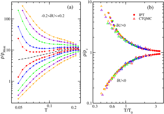
Figure 2: (a) DMFT resistivity curves as functions of the temperature along different trajectories across the Mott transition in a half-filled Hubbard model terletska-mott11prl. (b) Resistivity scaling displaying remarkable “mirror symmetry” gang4me.

Somewhat surprisingly, most DMFT studies of the Mott transition focused on the lowest temperature regime, paying little attention to the high temperature crossover regime relevant to many experiments. On the other hand, it is well known that at very low temperatures $T<T_{c}\sim 0.03T_{F}$, this model features a first order metal-insulator transition terminating at the critical end-point $T_{c}$ (Fig. 2), very similar to the familiar liquid-gas transition. For $T>T_{c}$, however, different crossover regimes have been tentatively identified georgesrmp but they have not been studied in any appreciable detail. The fact that the first order coexistence region is restricted to such very low temperatures provides strong motivation to examine the high temperature crossover region from the perspective of “hidden quantum criticality”. In other words, it is very plausible that the presence of a coexistence dome at $T<T_{c}\ll T_{F}$, an effect with very small energy scale, is not likely to influence the behavior at much higher temperatures $T\gg T_{c}$. In this high temperature regime smooth crossover is found, which may display behavior consistent with the presence of a “hidden” quantum critical (QC) point at $T=0$. To test this idea, very recent work terletska-mott11prl utilized standard scaling methods appropriate for quantum criticality and computed the resistivity curves along judiciously chosen trajectories respecting the symmetries of the problem. Characteristic scaling behavior for the entire family of resistivity curves has been identified, with the corresponding beta-function displaying striking “mirror symmetry” consistent with experiments. These findings provide compelling arguments in support of the suggestion that finite temperature behavior in many Mott systems should be interpreted from the perspective of quantum criticality christos-vlad05. It should stressed, however, that the DMFT solution in question does not contain any physical processes associated with approach to magnetic or charge ordering. If quantum criticality is indeed at play here, it has a fundamentally different nature, one that is associated with the destruction of a Fermi liquid without the aid of any static symmetry breaking pattern - in dramatic contrast to most known critical phenomena.

4 The disordered case

Let us now proceed to write down the equations for the dynamical mean field theory description of a disordered system janisvoll92,janisetal93,dk-prl93,dk-prb94. We will focus on the case of diagonal site disorder, which for the Hubbard model reads

$$H = -\sum_{\left\langle ij\right\rangle,\sigma}t_{ij}c_{i\sigma}^{\dagger}c_{j\sigma}+\sum_{j,\sigma}\varepsilon_{j}c_{j\sigma}^{\dagger}c_{j\sigma}+U\sum_{i}n_{i\uparrow}n_{i\downarrow},$$ (18)

where $\varepsilon_{j}$ are assumed to be independent random variables drawn from a given distribution $P\left(\varepsilon\right)$ whose strength is $W$ (say, a uniform distribution from $-W/2$ to $W/2$). Focusing once more on the local dynamics, it is clear it must now be dictated by

$$S_{eff}\left(j\right) = \sum_{\sigma}\int_{0}^{\beta}d\tau c_{j\sigma}^{\dagger}\left(\tau\right)\left(\partial_{\tau}+\varepsilon_{j}-\mu\right)c_{j\sigma}\left(\tau\right)$$ (19)

$$+ \sum_{\sigma}\int_{0}^{\beta}d\tau\int_{0}^{\beta}d\tau^{\prime}c_{j\sigma}^{\dagger}\left(\tau\right)\Delta\left(\tau-\tau^{\prime}\right)c_{j\sigma}\left(\tau^{\prime}\right)$$

$$+ U\int_{0}^{\beta}d\tau n_{j\uparrow}\left(\tau\right)n_{j\downarrow}\left(\tau\right).$$

Notice that the effective action is now different for different sites because of the $\varepsilon_{j}$ term. However, the hybridization function $\Delta\left(\tau\right)$ is not site-dependent. This is motivated again by the infinite-dimensional limit. Indeed, if the number of nearest-neighbors is infinite, the sum in Eq. (3) is effectively an averaging procedure over all possible realizations of the Green’s function. In fact, in the infinite-dimensional Bethe lattice, Eq. (11) becomes

$$\Delta\left(\tau\right) = zt^{2}\left[\frac{1}{z}\sum_{l=1}^{z}G_{ll}^{\left(j\right)}\left(\tau\right)\right]$$ (20)

$$\xrightarrow[z\to\infty]{} \tilde{t}^{2}\overline{G_{ll}\left(\tau\right)},$$ (21)

where the overbar denotes average over quenched disorder. Again, the effect of removing one nearest-neighbor is negligible in this case. Thus, the hybridization function is proportional to the average local Green’s function (see Fig. 1b and c). Solving the DMFT equations in the disordered case then entails solving an ensemble of single-impurity problems as in Eq. (19), one for each value of $\varepsilon_{j}$, and finding for each of them the local Green’s function and self-energy (which are now also site-dependent)

$$G_{jj}\left(\tau\right) = -\left\langle T\left[c_{j\sigma}\left(\tau\right)c_{j\sigma}^{\dagger}\left(0\right)\right]\right\rangle_{eff},$$ (22)

$$G_{jj}\left(i\omega_{n}\right) = \frac{1}{i\omega_{n}-\varepsilon_{j}+\mu-\Delta\left(i\omega_{n}\right)-\Sigma_{j}\left(i\omega_{n}\right)}.$$ (23)

The self-consistency can then be written, for the Bethe lattice, as (cf. Eqs. (11-13))

$$\Delta\left(i\omega_{n}\right)=\tilde{t}^{2}\overline{G_{jj}\left(i\omega_{n}\right)}=\tilde{t}^{2}\int d\varepsilon\frac{P\left(\varepsilon\right)}{i\omega_{n}-\varepsilon+\mu-\Delta\left(i\omega_{n}\right)-\Sigma\left[\varepsilon,i\omega_{n}\right]},$$ (24)

where we have slightly modified the notation in order to show that the denominator on the right-hand side depends on the site-energy $\varepsilon$ both explicitly and implicitly through the self-energy $\Sigma\left[\varepsilon,i\omega_{n}\right]$. It is obvious that the above procedure reduces to the original DMFT in the clean case (cf. Eq. (13)) but what does it reduce to in the non-interacting, disordered case?

It turns out that the treatment of disordered non-interacting systems obtained from these equations is equivalent to the so-called Coherent Potential Approximations (CPA) elliotetal74,EconomouCPA, which is known to become exact in infinite dimensions vlamingvollhardt92. The CPA equations are usually obtained through a strategy that consists in replacing the effects of scattering off the exact disorder potential by an effective average medium. Formally, one writes the average Green’s function in terms of an average medium self-energy $\Sigma_{AM}\left(i\omega_{n}\right)$ (a frequency-dependent complex quantity)

$$\overline{G\left(\boldsymbol{k},\boldsymbol{k}^{\prime},i\omega_{n}\right)}=\frac{\delta_{\boldsymbol{k},\boldsymbol{k}^{\prime}}}{i\omega_{n}-\varepsilon_{\boldsymbol{k}}+\mu-\Sigma_{AM}\left(i\omega_{n}\right)},$$ (25)

where again $\varepsilon_{\boldsymbol{k}}$ is the clean non-interacting dispersion. $\Sigma_{AM}\left(i\omega_{n}\right)$ is calculated by replacing the average medium by the exact potential (as defined by the actual values of $\varepsilon_{j}$) at a single generic site (while keeping it at the other sites) and imposing that the difference between the exact and the average scattering t-matrices vanishes on the average elliotetal74,EconomouCPA. A similar, effective medium approach, incidentally, can be used to derive the DMFT of clean interacting systems georgesrmp, so it is no surprise that one recovers CPA in this case. In the generic case of disordered interacting systems, $\Sigma_{AM}\left(i\omega_{n}\right)$ is obtained from the local part of the average Green’s function

$$\overline{G_{jj}\left(i\omega_{n}\right)} = \int d\varepsilon\frac{P\left(\varepsilon\right)}{i\omega_{n}-\varepsilon+\mu-\Delta\left(i\omega_{n}\right)-\Sigma\left[\varepsilon,i\omega_{n}\right]}$$ (26)

$$= \frac{1}{N_{s}}\sum_{\boldsymbol{k}}\frac{1}{i\omega_{n}-\varepsilon_{\boldsymbol{k}}+\mu-\Sigma_{AM}\left(i\omega_{n}\right)}.$$

One may wonder what is the form of the DMFT self-consistency for generic disordered interacting systems, beyond the Bethe lattice case, in other words, the analogue of Eq. (14). This is most easily done through the analogy with CPA. Once we have the local self-energy for every value of $\varepsilon_{j}$, $\Sigma_{j}\left(i\omega_{n}\right)$, for a given $\Delta\left(i\omega_{n}\right)$, Eqs. (22,23), we first find the average medium self-energy $\Sigma_{AM}\left(i\omega_{n}\right)$ through Eq. (26). We then note that the average local Green’s function within CPA is also given by

$$\overline{G_{jj}\left(i\omega_{n}\right)}=\frac{1}{i\omega_{n}+\mu-\Delta\left(i\omega_{n}\right)-\Sigma_{AM}\left(i\omega_{n}\right)},$$ (27)

since this is what you get if you replace the actual scattering potential $\varepsilon_{j}+\Sigma_{j}\left(i\omega_{n}\right)$ in Eq. (23) by the effective medium self-energy $\Sigma_{AM}\left(i\omega_{n}\right)$. Finally, from comparing Eqs. (26) and (27) we arrive at the desired self-consistency condition

$$\frac{1}{N_{s}}\sum_{\boldsymbol{k}}\frac{1}{i\omega_{n}-\varepsilon_{\boldsymbol{k}}+\mu-\Sigma_{AM}\left(i\omega_{n}\right)}=\frac{1}{i\omega_{n}+\mu-\Delta\left(i\omega_{n}\right)-\Sigma_{AM}\left(i\omega_{n}\right)},$$ (28)

which would give an improved hybridization function $\Delta\left(i\omega_{n}\right)$ in an iterative procedure. We should note in passing that the average medium self-energy and the average Green’s function (25) are the key ingredients in the calculation of the conductivity, which as mentioned before involves no vertex corrections within DMFT dk-prb94.

It is important to know what the limitations of this approach are. The main one is its inability to describe the disorder-induced Anderson metal-insulator transition anderson58. As the self-consistency condition makes quite apparent, the central order parameter of this mean field theory is the average local Green’s function, see Eqs. (21), (26) or (28). However, as explained by Anderson in the original 1958 paper anderson58, the average local Green’s function, which is non-critical and finite at the mobility edge, is unable to signal the phase transition between extended and localized states. Indeed, the spatial fluctuations of the local Green’s function are so large that its typical value is far removed from the average one (see Fig. 1b and c). Thus, DMFT cannot describe the Anderson localization transition and one needs to go beyond this approximation if Anderson localization effects are to be incorporated. It had long been known that CPA has no Anderson transition, so this should not come as a big surprise. We will show below, however, that one can in fact address the effects of localization, while at the same time retaining the local description of all correlation effects.

5 Applications of the disordered DMFT

Early applications of the disordered DMFT scheme focused on the phase diagram of the disordered Hubbard model. In particular, the fate of the antiferromagnetic phase of the clean model when disorder is introduced was investigated ulmkeetal95,singhetal98. Appropriate incorporation of broken symmetry phases, like antiferromagnetism, requires generalizing the procedure of Section 4 through the introduction of sub-lattice structure and spin-dependent single particle quantities, which is quite straightforward and will not be discussed here georgesrmp. The main findings are a surprising enhancement of the ordering tendencies at weak disorder and strong interactions, which was attributed to a peculiar disorder-induced delocalization effect ulmkeetal95,singhetal98. More recently, the phase diagram of the paramagnetic Hubbard model (suitable for systems with a high degree of magnetic frustration) has been determined, showing a gradual suppression of the region of coexistence of metallic and insulating phases found in the clean case aguiaretal05.

Kondo disorder

A very attractive feature of the disordered DMFT approach is its ability to provide full distributions of local quantities, which in turn may have profound effects on the low temperature behavior of physical systems. Consider for example the ensemble of effective actions in Eq. (19), which, as explained before, can be viewed as an ensemble of Anderson single-impurity problems, with the same conduction electron bath (Eq. (6)), but different impurity-site energies $\varepsilon_{j}$. As is well known, at sufficiently strong coupling $U$, a local magnetic moment can be stabilized at these impurity sites at high temperatures Anderson1961. However, below an energy scale set by the Kondo temperature $T_{Kj}$, the moments are “quenched” by the conduction electrons and form a singlet bound state (or Kondo resonance) Anderson1961,Kondo1964,Yuval-Anderson2,Yuval-Anderson1,Nozi‘eres1974,K.G.Wilson1975,Hewson1993. The dependence of $T_{Kj}$ on $\varepsilon_{j}$ is given by

$$T_{Kj}\approx D\exp\left(-1/\rho_{F}J_{j}\right),$$ (29)

where $D$ and $\rho_{F}$ are the conduction electron half band-width and density of states at the Fermi level, respectively, and $J_{j}$ is the local Kondo exchange coupling constant Schrieffer1966

$$J_{j}=2\left|V_{k_{F}}\right|^{2}\left[\frac{1}{\left|\varepsilon_{j}\right|}+\frac{1}{\left|\varepsilon_{j}+U\right|}\right].$$ (30)

Therefore, because of the strong exponential dependence of the Kondo temperature on the local parameters, a distribution of site energies can give rise to a wide distribution of Kondo temperatures Dobrosavljevi’c1992b. As a consequence, depending on whether a specific site has $T_{Kj}<T$ or $T_{Kj}>T$, it will behave as a free spin in the former case or as a quenched inert impurity in the latter one, with significant effects on thermodynamic and transport properties, see Fig. (3).

Figure 3: Distribution of Kondo temperatures for the alloys $\mathrm{UCu_{4}Pd}$ (long dashed line) and $\mathrm{UCu_{3.5}Pd_{1.5}}$ (short dashed line). Spins with $T_{K}$ in the hatched area ($T>T_{K}$) behave as effectively free and lead to a singular thermodynamic response. From reference mirandavladgabi1.

This scenario has received strong experimental support in the context of disordered heavy fermion systems. This was initially sparked by NMR experiments done on the Kondo alloy $\mathrm{UCu_{4-x}Pd_{x}}$, whose broad temperature-dependent line-widths were analyzed in terms of a distribution of Kondo temperatures Bernal1995. The same distribution was then used to calculate the magnetic susceptibility and the specific heat, with very good agreement with the observed behavior Bernal1995. In this context, this phenomenology has been dubbed the Kondo disorder model. This was particularly striking because this system was among many intensively studied heavy fermion compounds stewartNFL,Stewart2006 whose properties are in apparent contradiction with Landau’s theory of Fermi liquids Landau1957,Landau1957a,Landau1959. In particular, the magnetic susceptibility showed an approximately logarithmic divergence with lowering temperatures, in contrast with the usual saturation to a constant found in weakly, or even some strongly correlated Fermi liquid metals. The reason for the observed anomalous behavior was quite clear within the Kondo disorder model. Indeed, the distribution of Kondo temperatures needed to explain the NMR line-widths was so broad that $P\left(T_{K}\right)\approx P_{0}=\mathrm{const.}$ when $T_{K}<\Lambda$, where $\Lambda$ is some low energy scale of the distribution. In this case, no matter how low the temperature is, there are always a few unquenched spins left over with $T_{K}<T$ whose contribution to the susceptibility is Curie-like and large (Fig. (3))

$$\chi\left(T\right)\sim\frac{1}{T}.$$ (31)

Thus, by using a fairly accurate parametrization of the Kondo susceptibility K.G.Wilson1975

$$\chi_{Kondo}\left(T\right)\sim\frac{1}{T+\alpha T_{K}},$$ (32)

one can immediately find that the bulk susceptibility obtained from an average over the local contributions calculated with the empirical $P\left(T_{K}\right)$ distribution is dominated by the low-$T_{K}$ spins (with $T_{K}\ll T\sim\Lambda$) and is logarithmically divergent

$$\overline{\chi}\left(T\right)\sim\int\frac{P\left(T_{K}\right)}{T+\alpha T_{K}}dT_{K}\sim\int_{0}^{\Lambda}\frac{P_{0}}{T+\alpha T_{K}}dT_{K}\sim\ln\left(\frac{T_{0}}{T}\right),$$ (33)

where $T_{0}$ is a distribution-dependent constant.

Clearly, the Kondo disorder model found a natural setting within the DMFT approach to disordered systems, which put the phenomenology obtained from NMR on a firmer basis mirandavladgabi1,mirandavladgabi2,mirandavladgabi3. Because heavy fermion systems are characterized by a lattice of ions with incomplete f-shells, the most appropriate model Hamiltonian is a disordered Anderson lattice Hamiltonian

$$H_{And} = -\sum_{\left\langle ij\right\rangle,\sigma}t_{ij}c_{i\sigma}^{\dagger}c_{j\sigma}+\sum_{j,\sigma}\left(\varepsilon_{j}-\mu\right)c_{j\sigma}^{\dagger}c_{j\sigma}+\sum_{j,\sigma}\left(E_{fj}-\mu\right)f_{j\sigma}^{\dagger}f_{j\sigma}$$ (34)

$$+ \sum_{j,\sigma}\left(V_{j}c_{j\sigma}^{\dagger}f_{j\sigma}+\mathrm{H.c.}\right)+U\sum_{j}f_{j\uparrow}^{\dagger}f_{j\uparrow}^{\phantom{\dagger}}f_{j\downarrow}^{\dagger}f_{j\downarrow}^{\phantom{\dagger}},$$

in usual notation, and in which we have in general assumed that both f- and c-site energies, $E_{fj}$ and $\varepsilon_{j}$, as well as the local hybridizations $V_{j}$ between them are random quantities, each with its own independent distribution. The effective local action in this case reads

$$S_{eff}\left(j\right) = \int_{0}^{\beta}d\tau\sum_{\sigma}\left[c_{j\sigma}^{\dagger}\left(\tau\right)\left(\partial_{\tau}+\varepsilon_{j}-\mu\right)c_{j\sigma}\left(\tau\right)+f_{j\sigma}^{\dagger}\left(\tau\right)\left(\partial_{\tau}+E_{fj}-\mu\right)f_{j\sigma}\left(\tau\right)\right]$$ (35)

$$+ \int_{0}^{\beta}d\tau\int_{0}^{\beta}d\tau^{\prime}\sum_{\sigma}\left[c_{j\sigma}^{\dagger}\left(\tau\right)\Delta\left(\tau-\tau^{\prime}\right)c_{j\sigma}\left(\tau^{\prime}\right)\right]$$

$$+ \int_{0}^{\beta}d\tau\left[V_{j}\sum_{\sigma}c_{j\sigma}^{\dagger}\left(\tau\right)f_{j\sigma}\left(\tau\right)+Uf_{j\uparrow}^{\dagger}\left(\tau\right)f_{j\uparrow}\left(\tau\right)f_{j\downarrow}^{\dagger}\left(\tau\right)f_{j\downarrow}\left(\tau\right)\right],$$

and the self-consistency condition is analogous to the one in Eq. (24)

$$\Delta\left(i\omega_{n}\right)=\tilde{t}^{2}\overline{G_{jj}^{c}\left(i\omega_{n}\right)},$$ (36)

where the local $c$-electron Green’s function $G_{jj}^{c}\left(i\omega_{n}\right)$ is

$$\left[G_{jj}^{c}\left(i\omega_{n}\right)\right]^{-1}=i\omega_{n}-\varepsilon_{j}+\mu-\frac{V_{j}^{2}}{i\omega_{n}-E_{fj}-\Sigma_{j}\left(i\omega_{n}\right)}-\Delta\left(i\omega_{n}\right),$$ (37)

and the averaging procedure is performed over the random quantities $\varepsilon_{j}$, $V_{j}$ and $E_{fj}$. Thus, $T_{K}$ fluctuations can have several origins in general, as the local Kondo temperature is affected by $\varepsilon_{j}$, $E_{fj}$ and $V_{j}$. Within DMFT, it was possible to better justify the ad hoc assumptions of the Kondo disorder model. In particular, one could quantify the validity of and thus justify the approximation of calculating the bulk susceptibility as an average over single-site contributions mirandavladgabi1. In addition, good agreement was also found with the dynamic magnetic susceptibility obtained through neutron scattering experiments Aronson1995. Furthermore, going well beyond the simple Kondo disorder phenomenology, the DMFT approach is able to give direct information about transport properties. It was found that mirandavladgabi1,mirandavladgabi2,mirandavladgabi3

• There is a strong interaction-induced renormalization of the disorder seen by the conduction electrons.

• This, in turn, leads to a rapid suppression of the low-temperature Fermi liquid coherence characteristic of clean heavy fermion materials, as a function of increasing disorder.

• Finally, when the quasi-particle coherence is completely destroyed and the distribution of Kondo temperatures develops a finite intercept in the limit of $T_{K}\to 0$, the non-Fermi liquid thermodynamics described above is accompanied by a non-Fermi liquid linear in $T$ resistivity

  $$\rho\left(T\right)=\rho_{0}-AT,$$ (38)

  where $A>0$. Like in the case of the thermodynamic properties, the anomalous resistivity is also due to left-over low-$T_{K}$ free spins off which the conduction electrons scatter incoherently.

It was possible to verify that the self-consistency does not lead to a large disorder dependence of the hybridization function $\Delta\left(\tau\right)$. As a result, the distribution of Kondo temperatures is fairly sensitive to the bare distribution of random parameters $\varepsilon_{j}$, $E_{fj}$ and $V_{j}$. Going beyond DMFT, as we will discuss later, one finds that this is an artifact of the approximations and, in general, self-consistency leads to a much more robust dependence on disorder.

Elastic and inelastic scattering in the disordered Hubbard model

The interplay between local correlation effects and transport is a striking feature which is made almost obvious by the DMFT scheme. This has been demonstrated in studies of the disordered Hubbard model, Eq. (18), in references Tanaskovi’c2003 and Aguiar2004, as we now describe.

The first study Tanaskovi’c2003 was confined to $T=0$ and thus addresses only the effects of elastic scattering. This was done using the Kotliar-Ruckenstein slave boson mean field theory as the impurity solver kotliarruckenstein (see Section 2 for further details). The relevant question is how interactions renormalize the scattering of quasiparticles by the disorder potential at the Fermi level (hence at $T=0$). In Hartree-Fock theory, the renormalized disorder potential is determined by the self-consistently determined distribution of the electronic charge. This, in turn, is governed by the charge compressibility if the charge can be assumed to readjust itself to the disorder potential in a fashion dictated by linear response theory. For small $U$, the response is that of a good metal and allows for a flexible adjustment of the charge to the bare random potential, leading to a weakened renormalized disorder (“disorder screening”) Herbut2001. For strong interactions close to Mott localization, however, the charge compressibility is significantly reduced (the metal becomes increasingly less compressible) and Hartree-Fock theory predicts poor disorder screening.

It was shown in Tanaskovi’c2003 that indeed the efficient disorder screening predicted by Hartree-Fock theory is recovered by DMFT at weak interactions. However, it was found that another phenomenon intervenes and strong disorder screening does occur even as the system approaches the Mott transition. The reason why this happens is once again related to the peculiarities of the Kondo effect discussed above. Indeed, as several DMFT studies have shown georgesrmp, the Mott transition is signaled by the disappearance of the metallic quasiparticles Brinkman1970. The coherent nature of these quasiparticles exists only within a narrow energy range around the Fermi level whose width is set by the Kondo temperature of the associated single-impurity problem: as $U\to U_{c}$, $T_{K}\to 0$. In the disordered case, there is a distribution of $T_{K}$’s, but all of them vanish at the transition. Now, the value assumed by the renormalized disorder potential on a given site is set by the position of the local Kondo resonances (within DMFT), which are known to be strongly pinned to the Fermi level Hewson1993. Therefore, Kondo resonance pinning strongly reduces the bare disorder fluctuations and screens the disorder rather effectively, leading to a correlation-induced suppression of the renormalized disorder, in sharp contrast to the simple Hartree-Fock prediction.

Kondo physics again comes in when one looks at inelastic scattering Aguiar2004. This was done by means of iterative perturbation theory georgeskotliar92,X.Y.Zhang1993,kajuetergabi (see Section 2 for more details). Indeed, $T_{K}$ governs also the temperature above which inelastic scattering dominates over elastic scattering. It is found that a gradual and mild temperature dependence of the resistivity is observed in the weakly correlated regime $U\approx W\ll D$, which is reasonably captured by Hartree-Fock theory. As interactions become of the order of (or larger than) the Fermi energy $U\approx W\gg D$, however, a sharper temperature dependence sets in. This is due to the strong suppression of the low-temperature scales of the associated Kondo impurity problems, which is not well described within Hartree-Fock theory.

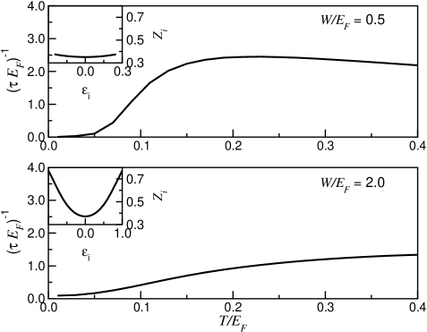
Figure 4: Scattering rate $1/\tau$ as a function of temperature for the disordered Hubbard model within DMFT at $U=2D\equiv 2E_{F}$ for weak ($W=0.5D$, top panel) and strong disorder ($W=2D$, bottom panel). Insets show the dependence of the local Kondo temperature $\sim Z_{i}$ on the site energy $\varepsilon_{i}$. At weak disorder, a sharp distribution of Kondo temperatures gives rise to a steep rise, whereas stronger disorder leads to a broad distribution and a slow temperature dependence. From reference Aguiar2004.

Furthermore, varying the disorder strength $W$ at strong interactions ($U\gg D$) leads to vastly different temperature dependences of the resistivity. Here, the distribution of Kondo temperatures defines the range over which inelastic processes become progressively more dominant. When $U\approx W$, a wide distribution of Kondo temperatures is generated and a rather slow growth of the resistivity with temperature is found. In contrast, in the cleaner case $W\ll U,$ there is a much narrower distribution of $T_{K}$’s resulting in a sharp temperature dependence of the resistivity, typical of the onset of coherence in heavy fermion materials Stewart1984 (see Fig. (4)).

2 Mott-Anderson transitions: Typical Medium Theory

Although the dynamical mean field theory described above is able to capture many features which are expected to be quite independent of its underlying assumptions (e. g., a distribution of local energy scales governing both thermodynamic and transport properties), it is clear its limitations call for improvements at several points. In particular, it would be highly desirable to incorporate Anderson localization effects. As we have seen, these are conspicuously absent in the original DMFT, as the latter is essentially a mean field theory whose order parameter is $\Delta\left(\omega\right)$, which in turn is determined by the average local Green’s function, see Eq. (24) or (27-28). As Anderson localization originates precisely in the spatial fluctuations of this quantity, this is not enough. Physically, $\Delta\left(\omega\right)$ represents the available electronic states to which an electron can “jump” on its way out of a given lattice site. From Fermi’s golden rule, the transition (“escape”) rate to a neighboring site is proportional to the imaginary part of $\Delta\left(\omega\right)$. If this is zero at the Fermi energy, the electrons cannot hop out and are effectively localized. In a clean system, in which this quantity is the same at every site, this is a good order parameter for localization, as in the case of the clean Mott transition. In a highly disordered system, $\Delta\left(\omega\right)$ shows strong spatial fluctuations from site to site and its average value is not a good measure of the conducting properties. A “typical” site in an Anderson insulator will have a hybridization function $\Delta_{i}\left(\omega\right)$ with large gaps and a few isolated peaks, reflecting the nearby localized wave functions that have an overlap with it. The vanishing of its imaginary part signals the electron’s inability to leave the site and is a good indicator of localized behavior. However, averaging over the whole sample washes out these gaps hiding the true insulating behavior. The discrepancy between the typical and average values of $\Delta_{i}\left(\omega\right)$ persists even on the metallic side, where $\Delta_{typ}\left(\omega\right)$ can be much smaller than $\overline{\Delta\left(\omega\right)}$.

Two alternative routes can be taken at this point. The ideal solution is to track the actual local hybridization or escape rate at each site. We will focus on this possibility in Section 3, where we analyze the so-called Statistical Dynamical Mean Field Theory. The other option is to focus on a simpler, yet meaningful measure of the escape rate which, though incapable of incorporating the richness of the actual local realizations, does not “throw away the (localization) baby with the bath water”. Here we should take as guidance the remark by Anderson that “no real atom is an average atom” andersonlocrev and seek a more apt description of a “real atom”. Indeed a good measure of the typical escape rate $\mathrm{Im}\Delta_{typ}\left(\omega\right)$ is the geometric average $\exp\left\langle\ln\left[\mathrm{Im}\Delta_{i}\left(\omega\right)\right]\right\rangle$. This has the great advantage of serving as an order parameter for the localization transition: indeed, in contrast to the algebraic average, the geometric average vanishes at the mobility edge anderson58 (see also M.Janssen1998,A.D.Mirlin2000,schubertetal10). We can then reason by analogy with the regular Dynamical Mean Field Theory approach explained above and construct a self-consistent extension centered around this typical escape rate function. This theory has been dubbed the Typical Medium Theory (TMT) tmt.

1 Formulation of the theory

We can proceed by analogy with the DMFT equations as explained in Section 4, see Eqs. (25-28), to obtain the Typical Medium Theory. We again focus on a disordered Hubbard model, Eq. (18), and imagine replacing the disordered medium by an effective typical medium described by a self-energy function $\Sigma_{TMT}\left(\omega\right)$. How do we determine this self-energy? Focusing on a generic site $j$, it is described by an effective action which has the same form as Eq. (19). The hybridization function $\Delta\left(\omega\right)$ is still left unspecified at this point, but we envisage that it will reflect a “typical” site as opposed to an “average” one, so we set $\Delta\left(\omega\right)=\Delta_{typ}\left(\omega\right)$ in Eq. (19). The local Green’s function is still defined as in Eqs. (22) and (23). The local density of states is given by the imaginary part of the local Green’s function

$$\rho_{j}\left(\omega\right)=\frac{1}{\pi}\mathrm{Im}G_{jj}\left(\omega-i\delta\right).$$ (39)

The typical local density of states can be defined through its geometric average

$$\rho_{typ}\left(\omega\right)=\exp\left[\int d\varepsilon_{j}P\left(\varepsilon_{j}\right)\ln\rho_{j}\left(\omega\right)\right].$$ (40)

Note that we have reverted to the real frequency axis because we need a positive-definite quantity in order to be able to define a geometric average. To preserve causality, the typical local Green’s function is obtained through the usual Hilbert transform

$$G_{typ}\left(\omega\right)=\int_{-\infty}^{\infty}d\omega^{\prime}\frac{\rho{}_{typ}\left(\omega^{\prime}\right)}{\omega-\omega^{\prime}}.$$ (41)

Note the analogous average quantity in the second equality of Eq. (26), which appears in DMFT. The typical medium self-energy $\Sigma_{TMT}\left(\omega\right)$ is then defined through the inversion of the following equation

$$G_{typ}\left(\omega\right)=\frac{1}{N_{s}}\sum_{\boldsymbol{k}}\frac{1}{\omega-\varepsilon_{\boldsymbol{k}}+\mu-\Sigma_{TMT}\left(\omega\right)},$$ (42)

which is the analogue of the first equality in Eq. (26). Finally, the loop is closed by setting

$$G_{typ}\left(\omega\right)=\frac{1}{\omega+\mu-\Delta_{typ}\left(\omega\right)-\Sigma_{TMT}\left(\omega\right)},$$ (43)

which can be used in an iterative scheme to generate an updated hybridization function $\Delta_{typ}\left(\omega\right)$ and is the analogue of Eq. (28). It becomes clear that the crucial difference between TMT and DMFT is the replacement of the average local Green’s function by the typical one (see Fig. 1b and c). This has been shown to capture even quantitative features of the Anderson localization transition, as we will discuss below. For a more comprehensive review, see TMTbook.

2 Applications of TMT

We will now describe the most important results obtained from the TMT theory of disordered systems. We will focus on the non-interacting case in Section 2 and on the disordered Hubbard model in Section 2. We should also mention a study of the Falicov-Kimball model within TMT in reference Byczuk2005a.

Critical behavior in the non-interacting case

As a first test of the usefulness of the TMT approach, it was first applied to the non-interacting three-dimensional case, Eq. (18) with $U=0$ tmt. In fact, the results of applying the TMT equations to a cubic lattice were directly compared to a numerical diagonalization of the Hamiltonian. In particular, the numerically determined arithmetic and geometric averages of the local density of states at the Fermi level, $\rho_{av}\left(\omega=0\right)$ and $\rho_{geo}\left(\omega=0\right)$, were compared to the results of CPA elliotetal74,EconomouCPA and of TMT (see Fig. 5). A remarkably accurate agreement between $\rho_{av}\left(\omega=0\right)$ and CPA was observed. As is known, this quantity is not critical at the Anderson transition. On the other hand, the geometric average of the local density of states does vanish at a critical disorder strength $W_{c}$. A reasonably good agreement between the numerical $\rho_{geo}\left(\omega=0\right)$ and TMT is found for most values of the disorder strength, even though TMT misses the correct critical behavior. This is not too surprising as TMT has the flavor of a mean field theory. Physically, it is clear the $\rho_{geo}\left(\omega\right)$ should be viewed as the density of extended states of system, decreasing with increasing disorder and eventually vanishing altogether for sufficiently large randomness. Thus, the spectral weight described by $\rho_{geo}\left(\omega\right)$ is not conserved.

In fact, further insight into the critical behavior of TMT can be achieved analytically tmt. By assuming an elliptic density of states for the clean lattice, $\rho_{0}\left(\omega\right)=\frac{2}{\pi D}\sqrt{1-\left(\frac{\omega}{D}\right)^{2}}$, it can be proved that in the critical region $W\to W_{c}=eD$, the typical density of states (given, as usual, by the geometric average) assumes a universal form

$$\rho_{typ}\left(\omega,W\right)\approx\rho\left(\omega=0,W\right)f\left[\omega/\omega_{0}\left(W\right)\right],$$ (44)

where

$$\rho\left(\omega=0,W\right)=\left(\frac{4}{\pi}\right)^{2}\left(W_{c}-W\right),$$ (45)

the frequency scale

$$\omega_{0}\left(W\right)=\sqrt{\frac{e}{4}\left(W_{c}-W\right)},$$ (46)

and the scaling function has a simple form $f\left(x\right)=1-x^{2}$. Note that Eq. (45) gives an order parameter critical exponent $\beta_{TMT}=1$, which should be compared to the accepted value in three dimensions $\beta_{3D}\approx 1.58$ slevinohtsuki99.

Figure 5: Comparison between the TMT and CPA with numerical results (circles) on the non-interacting 3D tight-binding model with diagonal disorder. The average local density of states at the band center $\rho_{av}$ is remarkably well captured by the Coherent Potential Approximation (dashed line) but is not critical at the Anderson localization transition at $W_{c}\approx 1.38$ (in units of the clean bandwidth). The geometrically averaged local density of states $\rho_{typ}$, on the other hand, vanishes at the transition and is well described by the Typical Medium Theory (full line), except for the detailed critical behavior. The inset shows the numerics for the critical behavior of $\rho_{typ}$ as a function of the correlation length $\xi\left(W\right)$, where $\xi\left(W\right)\sim\left|W-W_{c}\right|^{\nu}$, $\nu\approx 1.58$. From reference tmt.

The disordered Hubbard model at half filling

We now direct our attention to disordered interacting systems. The TMT was applied to the disordered Hubbard model byczuketal05,aguiaretal09. The phase diagram of the paramagnetic half-filled case at $T=0$ was obtained with two different impurity solvers: Wilson’s numerical renormalization group (NRG) K.G.Wilson1975 was used in byczuketal05 and the Kotliar-Ruckenstein slave boson mean field theory (SB4) kotliarruckenstein was applied in aguiaretal09. The results obtained largely agree with each order but there are some small discrepancies in the details. Essentially, three different phases are observed: a disordered correlated metal phase, characterized by $\rho_{c}\equiv\rho_{typ}\left(\omega=0\right)\neq 0$, a Mott-like insulating phase (which we will call simply a Mott insulator) and a Anderson-like insulating phase (for which we will use the name Mott-Anderson insulator), the latter two phases having $\rho_{c}=0$. We will discuss each set of results and then the discrepancies. For reviews, see TMTbook and byczuketal10.

For small values of disorder and interaction, both approaches find that the system is metallic, although this is not too surprising. There is also agreement on the fact that, for a fixed small disorder strength, the order parameter $\rho_{c}$ increases with increasing interaction ($U>W$). This is a reflection of disorder screening by interactions (see Section 5). Eventually, at a critical value of the interaction strength $U_{c}\left(W\right)$, the order parameter $\rho_{c}$ exhibits a finite jump and drops to zero, signaling a metal-Mott insulator phase transition. Furthermore, both methods agree that, for a fixed small value of $U$, as one increases the disorder ($W>U$) $\rho_{c}$ decreases monotonically, indicating that the spectral weight due to extended states is decreasing. At the critical value $W_{c}\left(U\right)$, $\rho_{c}$ vanishes and the system enters a Mott-Anderson insulating phase.

The differences in the results of the two approaches are the following. The NRG-based TMT byczuketal05 predicts the metal-Mott insulator transition for $U>W$ to be first order in character, with typical hysteretic behavior: the metallic solution is locally stable for $U<U_{c2}\left(W\right)$ and the Mott-insulating solution is locally stable for $U>U_{c1}\left(W\right)$, where $U_{c1}\left(W\right)<U_{c2}\left(W\right)$. In the coexistence region $U_{c1}\left(W\right)<U<U_{c2}\left(W\right)$, both solutions can be stabilized (although only one is a true global energy minimum at each $U$). The SB4-based TMT aguiaretal09, on the other hand, predicts no hysteresis. To understand this, it should be mentioned that SB4 is a good description of the low-energy properties of the impurity spectral function, although it misses the higher-energy features which give rise to the Hubbard bands in the lattice. An important ingredient of this description is the quasiparticle weight $Z_{i}\equiv Z\left(\varepsilon_{i}\right)$, well known from Fermi liquid theory, which in the impurity problem - Eq. (19) - determines the width of the Kondo resonance (essentially the Kondo temperature). Formally, it appears in the local Green’s function at site $i$

$$G_{ii}\left(i\omega_{n}\right)=\frac{Z_{i}}{i\omega_{n}-\tilde{\varepsilon}_{i}+\mu-Z_{i}\Delta_{typ}\left(i\omega_{n}\right)},$$ (47)

where $\tilde{\varepsilon}_{i}$ is the renormalized local site energy, which gives the position of the resonance. In the clean lattice case, $Z$ vanishes continuously as the interaction strength is tuned to its critical value $U\to U_{c}$, $Z\sim U_{c}-U\to 0$, signaling the Mott localization of the itinerant electrons, which become localized magnetic moments. The continuous nature of the transition in the clean case, with no accompanying hysteresis, survives the introduction of disorder within the SB4-based TMT. In fact, in this approach all the $Z_{i}$’s vanish at a unique $U_{c}\left(W\right)$. It should be stressed that in both approaches $\rho_{c}$ is discontinuous at the transition, a fact which can be ascribed (at least for small disorder) to the observed perfect screening of disorder ($\rho_{av}\left(\omega=0\right)\to\rho_{geo}\left(\omega=0\right)$ as $U\to U_{c}\left(W\right)$) and the pinning of the clean density of states at the Fermi level to its non-interacting value (see Section 5).

Moreover, the results obtained with the NRG impurity solver indicate that the transition in the region $W>U$ is such that $\rho_{c}\to 0$ continuously as $W\to W_{c}\left(U\right)$ byczuketal05. This is in contrast to the SB4-based approach, which finds that $\rho_{c}$ exhibits a discontinuous jump to zero at $W_{c}\left(U\right)$ aguiaretal09. In fact, the latter method brings out an important ingredient which significantly enhances the physical understanding of the TMT approach to this problem. This is achieved by tracking the behavior of the quasiparticle weights $Z_{i}$. For a given fully-converged hybridization function $\Delta_{typ}\left(i\omega_{n}\right)$, the ensemble of impurity problems is characterized by the function $Z\left(\varepsilon_{i}\right)$ for $\left|\varepsilon_{i}\right|<W/2$ (a uniform disorder distribution is assumed). This function has the property that, as the phase transition is approached, $Z\left(\varepsilon_{i}\right)\to 0$ for $\left|\varepsilon_{i}\right|<U/2$, whereas $Z\left(\varepsilon_{i}\right)\to 1$ if $\left|\varepsilon_{i}\right|>U/2$ (see Fig. 6) aguiaretal06. In the SB4 language kotliarruckenstein, $Z\to 0$ implies a singly occupied site with a localized magnetic moment, whereas $Z\to 1$ means either a doubly occupied or a singly occupied site, either of which is essentially non-interacting. Thus, in the region $W>U$, a fraction of the sites, those with $\left|\varepsilon_{i}\right|<U/2$, experience Mott localization, while those sites with $\left|\varepsilon_{i}\right|>U/2$ undergo Anderson localization. The picture that emerges is that of a spatially inhomogeneous system, composed of Mott-localized droplets intermingled with Anderson insulating regions. This situation has been dubbed a “site-selective Mott transition” aguiaretal09. Analytical insight into the SB4-results can be brought to bear in order to show that in that approach any finite $U$ renders the vanishing of $\rho_{c}$ discontinuous, in sharp contrast to the non-interacting case tmt.

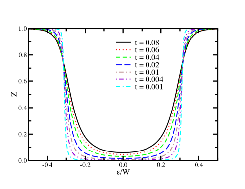
Figure 6: $Z\left(\varepsilon_{i}\right)$ showing the two-fluid behavior of the Mott-Anderson transition within TMT. As the transition is approached ($t\to 0$) for $W=2.8>U=1.75$, sites with $\left|\varepsilon_{i}\right|<U/2\approx 0.31W$ represent Mott insulating regions with $Z\left(\varepsilon_{i}\right)\to 0$, whereas sites with $\left|\varepsilon_{i}\right|>U/2$ are Anderson localized with $Z\left(\varepsilon_{i}\right)\to 1$. From reference aguiaretal06.

Finally, in the intermediate region of $W\approx U$, it was suggested, based on the NRG results that there might be a crossover from a metal to a disordered Mott insulator byczuketal05. However, since their results clearly show regions where $\rho_{c}\neq 0$ and regions where $\rho_{c}=0,$ we believe the correct interpretation is to identify the former as metallic and the latter as insulating. Besides, this is expected from the sharp distinction between an insulator and a metal at zero temperature. Having said that, however, it is clear that the nature of the transition in this problematic region certainly deserves a further more detailed investigation.

The disordered Hubbard model was also studied within TMT by allowing antiferromagnetic order on a bipartite lattice byczuketal09. The phase diagram at zero temperature as a function of disorder and interactions was determined, with the identification of both paramagnetic and antiferromagnetic metallic phases (for finite disorder only), an antiferromagnetic Mott insulating phase and a paramagnetic Anderson insulating phase at large disorder strength.

3 Mott-Anderson transitions: Statistical DMFT

As outlined above, the most natural and accurate extension of the DMFT philosophy which can incorporate Anderson localization effects is one which replaces the algebraic average of the hybridization function $\overline{\Delta\left(\omega\right)}$ (as in the original DMFT) or its typical value/geometric average $\Delta_{typ}\left(\omega\right)$ (as in the TMT), by the actual realizations of $\Delta_{j}\left(\omega\right)$ at each site motand,london (see Fig. 1b and c). As is to be expected, the complexity of the equations increases considerably and one has to rely heavily on numerical computations. However, many insights have been obtained regarding the systems analyzed. Besides, a much larger degree of universality of the distributions is observed when compared with the much more “rigid” approaches of DMFT or TMT.

1 Formulation of the theory

Let us examine how the statDMFT works. We begin with the by now familiar disordered Hubbard model of Eq. (18) and focus, as usual, on the dynamics of a given site $j$, dictated by an effective action (we now revert back to imaginary time)

$$S_{eff}\left(j\right) = \sum_{\sigma}\int_{0}^{\beta}d\tau c_{j\sigma}^{\dagger}\left(\tau\right)\left(\partial_{\tau}+\varepsilon_{j}-\mu\right)c_{j\sigma}\left(\tau\right)$$ (48)

$$+ \sum_{\sigma}\int_{0}^{\beta}d\tau\int_{0}^{\beta}d\tau^{\prime}c_{j\sigma}^{\dagger}\left(\tau\right)\Delta_{j}\left(\tau-\tau^{\prime}\right)c_{j\sigma}\left(\tau^{\prime}\right)$$

$$+ U\int_{0}^{\beta}d\tau n_{j\uparrow}\left(\tau\right)n_{j\downarrow}\left(\tau\right).$$

Notice the crucial difference now: the hybridization function $\Delta_{j}\left(i\omega_{n}\right)$ is now site-dependent. Each site, besides having a different energy $\varepsilon_{j}$, also “sees” a different local environment $\Delta_{j}\left(i\omega_{n}\right)$. The local dynamics is again encoded in a site-dependent self-energy $\Sigma_{j}\left(i\omega_{n}\right)$, obtained from the local Green’s function as before, see Eqs. (22) and 23). It is important to note that this description assumes a diagonal (albeit site-dependent) self-energy function, adhering to the generic philosophy of incorporating only local interaction effects.

Unlike the previous DMFT or TMT approaches, statDMFT does not try to mimic this self-energy function $\Sigma_{j}\left(i\omega_{n}\right)$ through any type of effective medium. Instead, we choose to include its full spatial fluctuations. We do so by appealing to the physical picture of the self-energy as a shift of the local site energy, albeit a complex, frequency-dependent one: $\varepsilon_{j}\to\varepsilon_{j}+\Sigma_{j}\left(i\omega_{n}\right)$. Single-particle propagation can thus be viewed as described by the effective resolvent

$$\widehat{G}\left(i\omega_{n}\right)=\left[i\omega_{n}\widehat{1}-\widehat{t}-\widehat{\varepsilon}-\widehat{\Sigma}\left(i\omega_{n}\right)\right]^{-1},$$ (49)

where $\widehat{1}$ is the identity operator, $\widehat{t}$ and $\widehat{\varepsilon}$ are, respectively, the hopping and site-energy terms (first and second terms of the Hamiltonian (18)), and the matrix elements of the self-energy operator $\widehat{\Sigma}\left(i\omega_{n}\right)$ are given in the site basis as

$$\left\langle i\left|\widehat{\Sigma}\left(i\omega_{n}\right)\right|j\right\rangle=\Sigma_{j}\left(i\omega_{n}\right)\delta_{ij}.$$ (50)

Although any matrix element of the resolvent (49), both intra- and inter-site, can in principle be calculated (which is important, for example, for a Landauer-type calculation of the conductivity), the self-consistency requires only the diagonal part, related to the local Green’s function

$$\left\langle j\left|\widehat{G}\left(i\omega_{n}\right)\right|j\right\rangle=G_{jj}\left(i\omega_{n}\right)=\frac{1}{i\omega_{n}-\varepsilon_{j}-\Delta_{j}\left(i\omega_{n}\right)-\Sigma_{j}\left(i\omega_{n}\right)}.$$ (51)

This last equation closes the self-consistency loop by providing, in an iterative scheme, an updated hybridization function for each site $\Delta_{j}\left(i\omega_{n}\right)$. We summarize the self-consistency loop for completeness:

1. For a given realization of disorder, $\varepsilon_{j}$, start from a set of “initial trial” hybridization functions $\Delta_{j}\left(i\omega_{n}\right)$, one for each site.

2. For the set of effective actions (48), calculate the local Green’s function $G_{jj}\left(i\omega_{n}\right)$ (Eq. (22)) and the local self-energy $\Sigma_{j}\left(i\omega_{n}\right)$ (Eq. (23)) for each site.

3. Invert the matrix resolvent (49) and get its diagonal elements $G_{jj}\left(i\omega_{n}\right)$.

4. Obtain an updated set of hybridization functions $\Delta_{j}\left(i\omega_{n}\right)$ by equating these diagonal elements to the expression of the local Green’s functions, Eq. (51).

In general, the set of Eqs. (48-51) forms the so-called Statistical Dynamical Mean Field Theory of disordered correlated electron systems. It should be noted that, besides the challenge of solving the ensemble of impurity problems represented by Eq. (48), Eq. (51) poses the numerical problem of inversion of a complex matrix for each value of the frequency, which can be very time-consuming. The pay-off is a description which incorporates all Anderson localization effects. Indeed, when interactions are turned off, the theory becomes exact, since, e. g., Eq. (49) becomes the exact single-particle Green’s function (from which transport properties can be obtained with the Landauer formalism). In the absence of randomness, we recover, of course, the DMFT equations. In the presence of both disorder and interactions, this is the optimal theory of disordered interacting lattice fermions which includes only local correlation effects.

2 Early implementations of statDMFT: the Bethe lattice

It had long been known that the Bethe lattice (or “Cayley tree”) leads to considerable simplifications of the treatment of non-interacting disordered systems. For example, the so-called self-consistent theory of localization of Abou-Chacra, Anderson and Thouless abouetal becomes exact on a Bethe lattice. This is so because the local Green’s function with a neighboring site removed, Eq. (4), satisfies a single compact stochastic equation in that lattice, which allows for quite an efficient analysis, both analytically and numerically. It was shown, for example, that for a coordination number $z>2$, there is always an Anderson transition at a non-zero critical disorder strength $W_{c}$. This transition has been extensively studied mirlinfyodorov and is regarded as a large-dimensionality limit of the Anderson transition. Although it has an anomalous critical behavior, with an exponential rather than a power-law dependence, this description has been very fruitful, specially if one is interested in the non-critical region.

Given the complexity of the full statDMFT equations, this suggested that the preliminary investigations could be carried out on a Bethe lattice. Here, it is appropriate to comment on what is, in our view, a misunderstanding of the conceptual basis of the statDMFT approach. It has been stated semmleretal10b that there is somehow a conceptual difference between the statDMFT as applied to the Bethe lattice and the statDMFT used to analyze realistic lattices, like the square or cubic ones (for these, see the later Section 3). The misunderstanding comes from assuming that whereas on a realistic lattice one has a fixed disorder realization, which is then solved by statDMFT, therefore defining a deterministic problem, on the infinite Bethe lattice one does not deal with fixed disorder realizations but with distributions, and the approach becomes non-deterministic and “statistical” (we realize the origin of the misunderstanding may have been the use of this word in the name of the method london). This distinction is unfounded if one realizes that on any infinite lattice with a single fixed disorder realization (with random, spatially uncorrelated, parameters), the infinite values of local quantities (such as the local density of states) on each lattice site give rise to a statistical distribution of local quantities (assuming the lattice-translational invariance of the distributions, see lifshitzbook for a careful discussion). Thus, when one solves a given Hamiltonian with statDMFT on an infinite Bethe lattice, one is actually solving, in practice as well as in principle, for a single fixed disorder realization. Each iteration of the method outlined in abouetal corresponds to “going outwards” on the branches of a fixed disorder realization of an infinite Bethe lattice, while at the same time accumulating random variables and building a histogram of local quantities. By the same token, if one could solve the statDMFT equations for a single disorder realization on an infinite realistic (say, square) lattice, each one of its sites would contribute one random variable for a histogram of the same local quantities (which would be, obviously, different from the ones obtained from the differently connected Bethe lattice). In practice, of course, one solves many disorder realizations of finite, hopefully large, realistic lattices in order to generate distributions with good statistics. However, fundamentally, there is no conceptual difference between the statDMFT solutions on the two types of lattices.

The Mott-Anderson transition

In motand,london, the first implementation of the statDMFT theory, as applied to the Mott-Anderson transition described by the disordered Hubbard model was completed. This was done by using a Fermi liquid parametrization of the associated zero-temperature impurity problems, namely, the infinite-$U$ slave boson mean-field theory N.Read1983,colemanlong. Like its Kotliar-Ruckenstein finite-$U$ counterpart kotliarruckenstein, this theory captures the low energy sector and is known to give a quantitatively good description of this limit. This Fermi liquid description is encapsulated in just two parameters: the quasiparticle weight $Z_{j}$ and the effective level energy (or Kondo resonance location) $\tilde{\varepsilon}_{j}$. The local self-energy is written as

$$\Sigma_{j}\left(i\omega_{n}\right)=\left(1-Z_{j}^{-1}\right)i\omega_{n}+\frac{\tilde{\varepsilon}_{j}}{Z_{j}}-\varepsilon_{j}+\mu,$$ (52)

leading to a local Green’s function

$$G_{j}\left(i\omega_{n}\right)=\frac{Z_{j}}{i\omega_{n}-\tilde{\varepsilon}_{j}-Z_{j}\Delta_{j}\left(i\omega_{n}\right)}.$$ (53)

The results of motand,london reveal that, as in the non-interacting case, the Anderson-Mott transition can be identified by the vanishing of the typical local density of states (as described by the geometric average) at a certain critical disorder strength. Interestingly, in contrast to non-interacting electrons, the critical behavior is conventional (power-law) and the average density of states is divergent. There is at present no good understanding of this divergence.

Furthermore, a great opportunity afforded by statDMFT is the ability to investigate distributions of local quantities. By tracking the distribution of quasiparticle weights, it was found that it broadens considerably with increasing disorder, showing a characteristic power-law form at large randomness

$$P\left(Z\right)\sim Z^{\alpha-1},$$ (54)

with the exponent $\alpha=\alpha\left(W\right)$ a smooth function of disorder. It should be remembered that $Z_{j}$ determines the local Kondo temperature $T_{Kj}\sim Z_{j}$ and thus governs the local contribution to thermodynamic quantities such as the magnetic susceptibility and specific heat (see Section 5). In fact, by averaging over this distribution of $Z$’s as in Eq. (33), one finds power-law dependences for these quantities as well

$$\chi\left(T\right)\sim C\left(T\right)/T\sim T^{\alpha-1}.$$ (55)

As disorder increases, $\alpha$ decreases and eventually becomes smaller than 1 well before the Mott-Anderson transition. When this happens, the thermodynamic response becomes singular and non-Fermi liquid-like

$$\chi\left(T\to 0\right)\to\infty.$$ (56)

Many different correlated systems have indeed been shown to exhibit this form of anomalous behavior stewartNFL, with non-universal exponents $\alpha$. The presence of non-universal, smoothly varying exponents characterizing divergences in physical quantities is reminiscent of a large class of disordered systems and is usually dubbed a quantum Griffiths phase (for reviews, see Miranda2005,Vojta2006), by analogy with a similar situation in classical systems first analyzed by Griffiths griffiths. Most other known examples of quantum Griffiths phases had been found in the vicinity of magnetic phase transitions in the presence of disorder, most notably in insulating magnets D.S.Fisher92,D.S.Fisher95,guo-bhatt-huse-prb96,pichetal98,motrunichetal01, but also in metallic systems castronetoetal1,M.C.deAndrade1998,castroneto-jones-prb00,Millis2002. Here, however, the characteristic power laws are found in the vicinity of the paramagnetic Anderson metal-insulator transition and hence the name Electronic Griffiths phase was adopted. This anomalous behavior is apparently not at all dependent on the particular details of the disordered Hubbard model. Very similar power-law distributions of Kondo temperatures were also found in Bethe lattice implementations of statDMFT for the disordered Anderson lattice Hamiltonian (34) (see Fig. (7)) Miranda1999,Miranda2001,M.C.O.Aguiar2003.

Figure 7: Power-law distributions of Kondo temperatures in a disordered Anderson lattice model for different levels of disorder: the linear behavior for small values of $\log T_{K}$ implies a power-law $P\left(T_{K}\right)\sim T_{K}^{\alpha-1}$. The inset shows the exponent $\alpha$ as a function of disoder $W$. From reference Miranda2001.

It should be remembered that the forms of the distributions of Kondo temperatures obtained within DMFT were strongly dependent on the shape of the bare distributions of parameters. This is in sharp contrast to the ubiquitous power-law distributions found in the statDMFT approach. Thus, although the exponent $\alpha$ is disorder-dependent and non-universal, the power-law shape is quite independent of whether the bare parameters are given by, say, uniform, Gaussian or binary distributions M.C.O.Aguiar2003. This is again easy to understand if we note that the local Kondo temperature depends exponentially on the local density of states at the Fermi level (and less strongly on its value at higher energies). Now, due to the extended nature of the electronic wave functions in metallic systems, the density of states at one site is influenced by spatial fluctuations at very distant sites and thus samples a great number of local environments. The resulting distributions of local quantities thus reflect this long-distance sampling.

In order to understand why this effect leads specifically to a power law, an effective model was proposed in tanaskovicetal04. The effective model consisted of a disordered Anderson lattice model with Gaussian distributed conduction electron disorder ($\varepsilon_{j}$ in Eq. (34))

$$P\left(\varepsilon_{j}\right)=\frac{1}{\sqrt{2\pi}W}\exp\left(-\varepsilon_{j}^{2}/2W^{2}\right),$$ (57)

treated within DMFT. In DMFT, the hybridization function $\Delta\left(i\omega_{n}\right)$ is site-independent and the Kondo temperature distribution is solely determined by fluctuations of $\varepsilon_{j}$. It can then be shown that tanaskovicetal04

$$T_{Kj}=T_{K}^{0}e^{-\lambda\varepsilon_{j}^{2}},$$ (58)

where $T_{K}^{0}$ is the Kondo temperature at $\varepsilon_{j}=0$ and $\lambda$ is determined by other model parameters but does not depend on $\varepsilon_{j}$. It is easy to show from Eqs. (57) and (58) that

$$P\left(T_{K}\right)=P\left[\varepsilon_{j}\left(T_{K}\right)\right]\left|\frac{d\varepsilon_{j}}{dT_{K}}\right|\sim T_{K}^{\alpha-1},$$ (59)

which is precisely the power-law distribution of Kondo temperatures found generically within statDMFT treatments. We note, in passing, that this kind of argument is generic to all known quantum Griffiths phases: the relevant energy scales are exponentially suppressed by a certain random parameter (see Eq. (58)), whose probability is in turn also exponentially small (see Eq. (57)) Miranda2005,Vojta2006.

What is the relation between these results, obtained within DMFT, and the power laws observed in the applications of statDMFT? In statDMFT, the single (average) hybridization function of DMFT gets replaced by a strongly fluctuating distribution of local hybridizations $\Delta_{j}\left(i\omega_{n}\right)$. The imaginary part of each of these functions describes the available density of states for Kondo screening at site $j$ and enters the expression for the local Kondo temperature much like $\rho_{F}$ does in Eq. (29). From the central-limit theorem, fluctuations of the available densities of states around the mean value are generically Gaussian for weak and intermediate disorder and lead to a power-law distribution of $T_{K}$’s in a fashion quite similar to the effective model. Indeed, detailed calculations showed that the effective model is quite accurate when compared with full statDMFT results tanaskovicetal04. Crucially, these arguments can be used to show that the non-Fermi liquid behavior occurs already at quite moderate values of disorder and strictly precedes the Anderson metal-insulator transition. This elucidates then the microscopic origin of the electronic Griffiths phase.

Iterative perturbation theory as impurity solver

Most of the early statDMFT results on the Bethe lattice were obtained through the use of the infinite-U slave boson mean-field theory N.Read1983,colemanlong as impurity solver. These are good descriptions of the low-energy coherent Fermi-liquid part of the impurity spectrum but fail to account for inelastic scattering at low energies as well as higher-energy incoherent features such as upper and lower Hubbard bands. A technique which is able to incorporate there features is the so-called iterative perturbation theory georgeskotliar92,X.Y.Zhang1993,kajuetergabi. The iterative perturbation theory approach lends itself also more easily for an analysis of the temperature dependence of physical quantities. It has been used to analyze the disordered Anderson lattice model M.C.O.Aguiar2003 as well as the disordered Hubbard model semmleretal10. It suffers from the disadvantage of not being able to capture the correct exponential dependence of the low-energy Kondo scale, see Eqs. (29) and (58), leaving out, therefore, the possibility of characterizing Griffiths phase behavior (Section 2).

In the case of the disordered Anderson lattice, one of the interesting findings was the interplay between elastic scattering off the disorder potential and inelastic electron-electron scattering M.C.O.Aguiar2003. If one uses the inverse of the typical density of states at the Fermi level as a rough guide to the resistivity (a direct calculation of the resistivity was numerically prohibitive at the time of those studies), its temperature dependence is found to be quite sensitive to the amount of disorder. Indeed, low-disorder regimes are marked by an increase of the resistive properties with rising temperatures, signaling the onset of inelastic scattering processes, much like in the clean case. On the other hand, strongly disordered samples exhibit a decrease in the resistivity with increasing temperatures, because a decrease in the effective elastic scattering outweighs the increase in the inelastic one. This type of fan-like family of resistivity curves (see Fig. 8) has been seen in several disordered strongly correlated materials, being known as Mooij correlations mooij. They are seen to arise here within a local approach to electronic correlations and disorder.

Figure 8: Temperature dependence of the inverse typical conduction electron density of states of the disordered Anderson lattice model for different levels of disorder. This “fan-like” family of curves is generic to many disordered, strongly correlated systems (“Mooij correlations”). From reference M.C.O.Aguiar2003.

More recently the Hubbard model with binary alloy disorder has been also studied on a Bethe lattice with iterative perturbation theory as impurity solver semmleretal10. Particular attention has been paid to the dependence of the distribution of local densities of states on the small imaginary part (“broadening”) that is usually added to the frequency in numerical determinations of Green’s functions. The dependence of the distribution of local densities of states on this parameter can be used to characterize the localized or extended nature of the electronic states. The main result of that paper is the determination of the zero-temperature phase diagram of the model at a particular filling as a function of interaction and disorder strengths and the identification of regions with metallic, Mott-Anderson insulating and band insulating behaviors. In particular, the opening of the Mott gap occurs at values of the interaction and disorder strengths for which the gapless system is already Anderson localized. It is difficult to compare this phase diagram with the one obtained by the infinite-U slave boson mean field theory motand,london because the models were solved with different types of disorder and in different regimes.

3 StatDMFT on realistic lattices

Although the Bethe lattice implementations were very informative, its exotic connectivity introduces some unwanted features, especially with regard to the critical behavior of the Anderson transition mirlinfyodorov, which is believed to correspond to some infinite-dimensional limit. Therefore, it is important to check what the effects of finite dimensions are. Motivated by this, the full statDMFT equations have been implemented in realistic lattices in recent years. Given the successful application of DMFT to the description of the Mott-Hubbard transition, a natural candidate is the analysis of the disordered Mott-Hubbard transition.

The disordered Mott-Hubbard transition

As with any other phase transition, the characterization of the effects of disorder on the Mott transition poses an important yet difficult problem. In the particular case of phase transitions incontrovertibly described by an order parameter, this characterization has seen considerable advances. In insulating quantum magnets, many examples have been found in which a whole vicinity of the disordered critical point is described as a quantum Griffiths phase. This is a phase in which rare regions of nearly ordered material dominate the physics and the thermodynamic response becomes divergent Miranda2005,Vojta2006. The sizes and energy scales governing the rare regions span several orders of magnitude and their description requires taking account of very broad distributions. Furthermore, in many cases, as the critical point itself is approached, the relative widths of the distributions grow without limit, a situation generically described as an infinite randomness fixed point. This has been well established in systems with both Ising and continuous symmetry D.S.Fisher92,D.S.Fisher94,D.S.Fisher95,Hyman1996,yangetal,guo-bhatt-huse-prb96,Hyman1997,Fisher1998,pichetal98,narayanan-vojta-belitz-kirkpatrick-prl99,narayanan-vojta-belitz-kirkpatrick-prb99,motrunichetal01,G.Refael2002. More recently, a symmetry-based classification scheme of these Griffiths phases has been proposed and applied to several different systems with great success T.Vojta2003,vojta-schmalian-prb05,vojta-schmalian-prl05,Vojta2006,hoyos-vojta-prb06,hoyos-kotabage-vojta-prl07,hoyos-vojta-prl08,vojta-kotabage-hoyos-prb09. The Mott transition, however, poses a problem of a different nature, as it is not described by an order parameter in an obvious way. It is thus not clear how to extend the above insights into its description.

The implementation of statDMFT offers a natural way out. In particular, the clean problem is aptly described by DMFT, as we mentioned at the end of Section 2. The first implementation of statDMFT for the disordered Hubbard model was performed in songetal08 using the so-called “Hubbard I” (HI) approximation J.Hubbard1963 as the impurity solver. This simple impurity solver captures the physics close to the atomic limit and is therefore convenient for a study of the Mott insulating phase. However, it suffers from the deficiency of not giving rise to a quasiparticle peak in the single-impurity spectral function, a feature known to exist for any finite $U$ when the hybridization function is that of a good metal. The method was applied to the cases of half and quarter filling and the density of states and inverse participation ratio were obtained. Interestingly, the localization length has a non-monotonic behavior as a function of the interaction $U$: it increases initially with $U$, showing a tendency to delocalization, but eventually decreases and becomes even smaller than the non-interacting value at the Mott transition. At quarter filling, an Altshuler-Aronov B.L.Altshuler1979a density of states anomaly is found, which is however absent at half-filling, due to an interaction induced-suppression of the charge susceptibility.

Shortly afterwards, the disordered Hubbard model in a two-dimensional square lattice at $T=0$ was solved with statDMFT Andrade2009a,andrade09physicsB using the Kotliar-Ruckenstein slave boson mean field theory as the impurity solver kotliarruckenstein. Very similar results were also obtained pezzolietal09,pezzolietal10 within an approach based on a Gutzwiller variational wave function Gutzwiller1963,Gutzwiller1964,Gutzwiller1965. This is not too surprising, as the Kotliar-Ruckenstein theory, when applied to the Mott transition, is known to be equivalent to the Gutzwiller wave function approach. This kind of approach is known to be able to capture the low-energy features, such as the disappearance of the quasiparticle peak as the transition is approached, unlike the HI approximation. In the impurity problem language, the low-energy sector is described by two parameters, like in the infinite-$U$ case (see Section 2): the quasiparticle weight $Z$, well known from Fermi liquid theory, which determines the width of the Kondo resonance (essentially the Kondo temperature) and the resonance position $\tilde{\varepsilon}$, which measures its shift from the chemical potential. It is important to notice that in the clean lattice, $Z$ also determines the effective carrier mass ($m/m^{\ast}\sim Z$), a feature unique to cases in which the self-energy only depends on the frequency. Indeed, as the interaction strength is tuned to its critical value $U\to U_{c}$, $Z\sim U_{c}-U\to 0$, signaling the transmutation of the itinerant carriers into localized magnetic moments. In the statDMFT description, these local quantities vary from site to site, $Z\to Z_{i}$ and $\tilde{\varepsilon}\to\tilde{\varepsilon}_{i}$, and their distributions were thoroughly analyzed. Surprisingly, their critical behaviors were found to be very dissimilar.

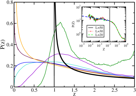
Figure 9: Power-law distributions of quasiparticle weights $Z$ in the half-filled disordered Hubbard model for different interaction strengths ($U/U_{c}\left(W\right)=0.6,0.8,0.9,0.92,0.94,0.97$) showing characteritic power-law behavior $P\left(Z\right)\sim Z^{\alpha-1}$: as $U\to U_{c}$, $\alpha\to 0$ and the curves become increasingly singular at small $Z$. The inset shows the weak dependence on the lattice size. From reference Andrade2009a.

As the transition is approached, which now happens at a disorder-dependent critical interaction $U_{c}\left(W\right)$, all $Z_{i}\to 0$, just like in the conventional Gutzwiller-Brinkman-Rice scenario. However, the quasiparticle weight distribution $P\left(Z\right)$ becomes increasingly broader as $U\to U_{c}\left(W\right)$. In fact, the typical value $Z_{typ}=\exp\left(\left\langle\ln Z\right\rangle\right)\to 0$, whereas the mean value remains finite, indicating that although almost all sites become local moments, some remain empty or doubly occupied aguiaretal06. Besides, the $Z$ distribution acquires a generic power-law shape, as in other Griffiths phases (see Fig. (9))

$$P\left(Z\right)\sim Z^{\alpha-1}.$$ (60)

This is very similar to the Bethe lattice studies of Section 2 and like in those cases, these power laws generate a singular thermodynamic response, see Eq. (55). Nevertheless, whereas before we had a disorder-driven Anderson-type transition, here this generic behavior is found in the proximity of the interaction-driven Mott transition for fixed disorder strength, clearly showing the amplifying effects of electronic correlations. The similarity to the quantum Griffiths scenario of magnets is not fortuitous. The low-$Z$ values which dominate the thermodynamics occur in exponentially rare regions of suppressed disorder. Finally, we note that just like in other known quantum Griffiths phases, this electronic Griffiths phase seems to be tied to a phase transition characterized by an infinite randomness fixed point: we find that, up to the numerical uncertainty, $\alpha\to 0$ as $U\to U_{c}\left(W\right)$.

Interestingly, correlations have the opposite effect on the distribution of resonance positions $\tilde{\varepsilon}_{i}$. Indeed, the width of the $\tilde{\varepsilon}$ distribution decreases as $U\to U_{c}\left(W\right)$ (see Fig. (10)). This is easily understood from the pinning of the Kondo resonances to the chemical potential, as already noted within DMFT Tanaskovi’c2003 (see Section 5). Just like in DMFT, this leads to a strong disorder screening effect, although, unlike in DMFT, here the screening effect is not perfect: a small amount of disorder seems to survive as the transition is approached.

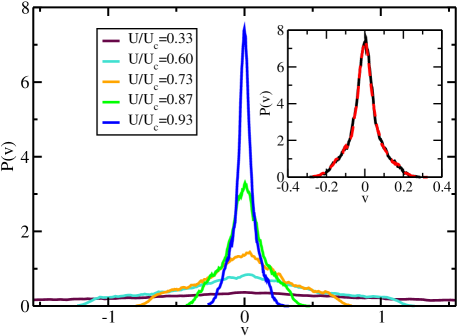
Figure 10: Distributions of the ratio of the local Kondo resonance position $\tilde{\varepsilon}_{i}$ to the quasiparticle weight $Z_{i}$, $v_{i}\equiv\tilde{\varepsilon}_{i}/Z_{i}$ in the half-filled disordered Hubbard model showing a decreasing effective disorder strength, as measured by $\tilde{\varepsilon}_{i}$, with increasing interactions. The inset shows the weak dependence on the lattice size (full line for $L=20$ and dashed line for $L=50$). From reference andrade09physicsB.

The disordered Hubbard model has also been investigated very recently in two dimensions with statDMFT and iterative perturbation theory as impurity solver semmleretal10. The disorder model used, however, was not the usual uniform diagonal disorder, but rather a combination of diagonal and off-diagonal disorder, together with disorder in the interaction term. This choice was intended to describe the so-called speckle disorder found in some set-ups of fermionic cold atoms loaded in optical lattices. The phase diagram was determined at half filling at zero as well as finite temperatures. A feature specific to this kind of disorder is the fact that it is unbounded and arbitrarily large values of on-site potentials occur. As a result, long (exponential) tails arise flanking the Hubbard bands which contribute to filling up a possible interaction-induced Hubbard gap. The main consequence of the presence of these tails is a partial suppression of the Mott insulating phase, in favor of a disordered strongly correlated metal phase. As a result, the Mott insulator and Anderson(-Mott) insulator phases do not share a phase boundary and are separated by a metallic phase. This is in contrast to the phase diagram obtained within TMT, see Section 2.

A single impurity in a strongly correlated host

The smallest element in an analysis of the effects of inhomogeneities in a crystal is a single isolated point-like impurity in an otherwise homogeneous host. In the case of a weakly correlated host, the expected effect is the formation of a potential scattering center, which can be usually be quite simply described at low energies by a set of phase shifts with a negligible temperature dependence. If the host is a weakly correlated metal, the localized impurity generates a radially oscillatory disturbance of the host charge. The oscillation is characterized by a wave vector determined by the extremal radii of the Fermi surface and an envelope which decays as the inverse of the distance to the impurity raised to the power $d$ in $d$ dimensions

$$\delta n\left(\boldsymbol{x}\right)\sim\frac{\cos\left(2k_{F}r\right)}{r^{d}}.$$ (61)

These are known as Friedel oscillations M.A.Ruderman1954,T.Kasuya1956,K.Yosida1957. A dilute collection of these impurities can then be treated as independent and their effects on transport properties is readily computed by conventional techniques, such as the Boltzmann equation.

The situation can be very different if the host is a strongly correlated system. The local inhomogeneity can disrupt the delicate balance of its host and lead to a spatially dependent pattern which has to be computed in a fully self-consistent manner. For example, local moments or antiferromagnetic ordering can be induced in the vicinity of the impurity allouletal09. Superconducting correlations, specially of the unconventional type (e. g., d-wave), also lead to characteristic spatial patterns in the vicinity of impurities, which can be probed by scanning tunneling microscopy (STM) techniques balatskyetal06. Besides, strong correlations typically generate very low energy scales. Therefore, one should expect a non-negligible energy and temperature dependence with possibly observable effects. Indeed, STM studies have revealed a non-trivial interplay between spatial fluctuations and the energy dependence of the local density of states in the cuprate superconductors McElroyetal05. In this case, the spectral function, probed by STM, is hardly affected by disorder up to the superconducting gap energy, whereas much stronger spatial fluctuations are observed at higher energies.

In general, the localized imperfection can be viewed as a source probe coupled to all wave vectors of the host charge. Therefore, if this coupling can be treated within linear response theory, the relevant quantity to keep track of is the host wave-vector-dependent charge susceptibility. The vicinity to the Mott metal-insulator transition causes the charge susceptibility to be strongly suppressed as the system becomes increasingly more localized. Therefore, we would expect considerable changes in the spatial pattern of the Friedel oscillations in a strongly correlated metal. The statDMFT is the tool of choice to study this situation. A single non-magnetic impurity in a half-filled Hubbard model has been studied using just such a tool andradeetal10. A great deal of analytical insight can then be obtained through an expansion in the disorder strength to first non-trivial order, using the Kotliar-Ruckenstein slave-boson impurity solver kotliarruckenstein. Note that the procedure is fully non-perturbative in the interaction strength. In the weak coupling limit, $U\ll D$, the approach has been shown to be fully equivalent to the Hartree-Fock approximation, which predicts a static self-energy

$$\Sigma_{j}\left(i\omega_{n}\right)=Un_{j}^{\left(0\right)},$$ (62)

where $n_{j}^{\left(0\right)}$ is the non-interacting charge density

$$n_{i}^{\left(0\right)}=1+2\Pi_{i0}^{\left(0\right)}V,$$ (63)

where $\Pi_{ij}^{\left(0\right)}$is the real-space static Lindhard polarization function and $V$ is the potential of the single impurity at site 0. This contains the usual Friedel oscillation pattern of Eq. (61).

However, as the interaction strength is tuned to be close to the Mott localization limit $U_{c}$, a very different situation arises. In this case, the charge density pattern decays as andradeetal10

$$n_{0}\approx-4\frac{\left(U_{c}-U\right)^{3}}{U_{c}^{5}}\left[\Pi^{\left(0\right)}\right]_{i0}^{-1}V\qquad\left(U\to U_{c}\right).$$ (64)

Two features of this result stand out. First, the spatial pattern is determined by the inverse of the static Lindhard function. Surprisingly, however, up to logarithmic corrections, the inverse static Lindhard function behaves very much the same as the usual Lindhard function. Second, the amplitude of the strongly-correlated Friedel oscillations is significantly suppressed as $U\to U_{c}$ down by the third power of the parametric distance to the transition. As a result, the charge perturbation dies out significantly as one recedes from the impurity, implying a short “healing length” (see Fig. 11). Comparison with numerical solutions of the statDMFT equations shows that the analytical expressions are quite accurate even for $\left|V\right|\lesssim D$.

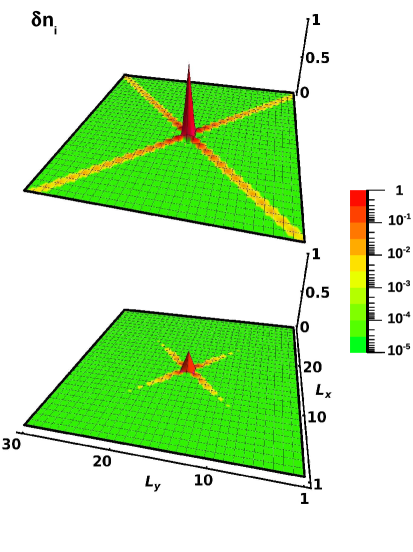
Figure 11: Friedel oscillation patterns of charge oscillations generated by a localized non-magnetic impurity in a half-filled Hubbard model. The long-ranged oscillations of $\delta n_{i}=n_{i}-1$ in the non-interacting case (top figure) are strongly suppressed in the strongly correlated regime (bottom figure, $m/m^{\ast}=0.3$). From reference andradeetal10.

The scattering T-matrix, which governs the transport properties, can also be computed with the same technique. We find its real space expression to be

$$T_{i}=\left[\delta_{i,0}+U\Pi_{i0}^{\left(0\right)}\right]V\qquad\left(U\ll U_{c}\right),$$ (65)

at small $U$ and

$$T_{i}=-\frac{U_{c}-U}{U_{c}^{2}}\left[\Pi^{\left(0\right)}\right]_{i0}^{-1}V\qquad\left(U\to U_{c}\right),$$ (66)

as one approaches the Mott transition. Here, the point to note is once again the strong suppression of scattering in the critical region, a situation by now already familiar (“disorder screening”).

The temperature dependence of the scattering is also very special. Indeed, it is known that the resistivity in the ballistic regime in two dimensions exhibits an anomalous, non-Fermi liquid linear in temperature dependence Zala2001, due to the coherent scattering off the Friedel oscillations created by the dilute impurities. Since we find these oscillations to be strongly suppressed by correlations it is important to study if the anomalous behavior survives. Besides, strong interactions also give rise to large inelastic scattering effects, and it is unclear if these are strong enough to mask the anomalous temperature dependence. The full analysis shows that andradeetal10:

• The interaction suppression of scattering (disorder screening), Eq. (66), acts to weaken both elastic and inelastic contributions from impurities, but does not destroy the non-Fermi liquid, anomalous behavior.

• However, inelastic scattering limits considerably the temperature range in which the linear in $T$ behavior of the resistivity is observed. These effects come both from the Friedel-oscillation regions, close to the impurities, as well as from the bulk, impurity-free regions of the system. It is found that, although both contributions are deleterious to the anomalous behavior, it is the bulk contribution which always dominates. In practice, even for quite modest mass renormalizations, the linear in $T$ regime is probably already unobservable: for $m/m^{\ast}\sim 0.6$, for example, it is restricted to $T\lesssim 10^{-4}T_{F}$, where $T_{F}\approx D$.

Both effects above seem to make the observation of the anomalous resistivity in two dimensions very unlikely in the strongly correlated regime.

In more general terms, the strategy of expansion in weak disorder strength outlined above, which is quite general, seems to be a good avenue for exploration of strongly correlated spatially inhomogeneous systems.

4 Inhomogeneous systems with slab geometries

Although the local approach outlined in Sections 1, 2 and 3 has been described in the context of random systems, its microscopic formulation motand,london is clearly applicable in any spatially non-uniform situation, whether random or not. Indeed, in the past several years this method has been applied to a number of non-random, yet spatially non-uniform systems. Because of this conceptual similarity, we chose to describe it here under the statDMFT “umbrella”, although the systems have nothing “statistical” in them. A particular focus has been put on systems composed of different materials arranged in a slab geometry. Motivation for these investigations has come both from advances in growth techniques of epitaxial heterostructures of complex materials, particularly transition metal oxides ohtomoetal02, and also from the use of surface sensitive probes of strongly correlated materials, such as photoemission experiments sekiyamaetal00,moetal03,rodolakisetal09. A number of different spatial arrangements of complex, strongly correlated materials have been considered: semi-infinite strongly correlated systems with a free-standing planar boundary (“strongly correlated surface physics”) potthoffnolting99,liebsch03,schwiegeretal03,borghietal09,borghietal10, planar interfaces between two semi-infinite materials Helmes2008, heterostructures okamotomillis04,okamotomillis04b, semi-infinite metallic leads sandwiching barriers of strongly correlated metals or insulators freericks04,chenfreericks07,zeniaetal09,borghietal10. Studies of other types of inhomogeneities have also been performed snoeketal08.

The abrupt change of chemical properties at the planes of surfaces or interfaces can lead to novel phenomena, some of which have been identified and characterized by the local approach we are describing here. This a fast moving area of research and we will not attempt to cover the richness of behavior that has been and continues to be uncovered. We will confine ourselves to a few important findings which serve to convey the flavor of these phenomena.

The interface between a metal and a Mott insulator

Metal-insulator and metal-semiconductor interfaces have been produced and studied for many years. Phenomena such as band bending due to charge rearrangement are well known. However, the question of what happens when a metal is grown epitaxially onto a Mott insulator has received much less attention. A first attempt to elucidate this question has been made by considering an ideal interface between particle-hole symmetric metallic and Mott insulating systems Helmes2008,borghietal09,borghietal10. In the absence of antiferromagnetism and within the DMFT picture, the spins of a bulk Mott insulator are not quenched because there are no conduction electrons available at the Fermi level with which they can form a singlet. When a Mott insulator is brought into contact with a metal, however, the layers which are closest to the interface can have access to the metallic carriers (through tunneling) and be quenched by means of the Kondo effect. This has been dubbed the “Kondo proximity effect”. Evidently, the metallization and Kondo quenching processes are established in a spatially smooth fashion as one enters the insulator, thus creating a strongly correlated metallic surface layer. The metallic character can be characterized by means of the by now familiar quasiparticle weight $Z\left(x\right)$, which is here a spatially varying quantity that depends on the distance $x$ from the interface. It is found that $Z\left(x\right)$ decays exponentially as a function of $x$

$$Z\left(x\right)\sim\exp\left(-x/\xi\right),$$ (67)

with a characteristic length scale $\xi$ which sets the size of the metallic surface layer and is determined by the parametric distance to the Mott transition, $\xi\sim\left(U_{c}-U\right)^{-1/2}$. The 1/2 value of the critical exponent is expected from the mean-field character of the approach. At Mott criticality, this characteristic length diverges and

$$Z\left(x\right)=\frac{A}{x^{2}}.$$ (68)

The numerical value of the constant $A$ above is found to be extremely small ($\sim 0.008$), showing the Kondo induced penetration of the metal into the Mott insulator to be extremely ineffective. The small values of the quasiparticle residues, which govern the local Fermi energy scale, also lead to a strong dependence on temperature, energy or applied voltage. Very small values of these perturbations are able to completely destroy the metallic behavior, leading to the concept of a “fragile” Fermi liquid zeniaetal09.

Surface dead layer

Another important phenomenon occurs at the free planar surface bounding a strongly correlated metal borghietal09,borghietal10. Here again the proximity to the interface with the vacuum induces variations of the quasiparticle residue $Z$. Interestingly, since the outermost layer electrons cannot tunnel further out of the material, they have less of a chance to hybridize and stabilize the metallic behavior. As a consequence, there is a strong suppression of the quasiparticle weight close to the open surface. In effect, the outermost electrons are a very “fragile” Fermi liquid if not completely Mott localized, thus creating a surface layer of almost Mott insulating character, the so-called “dead layer”. Once again the characteristic width of this layer also depends on the proximity to criticality as $\xi\sim\left(U-U_{c}\right)^{-1/2}$.

This has important consequences for the interpretation of photoemission experiments. For a long time, a quasiparticle peak had been sought in the photoemission spectra of strongly correlated materials with little success. While there have been many attempts to explain this mystery, it is clear now that one expects on general grounds that the quasiparticle peak width (which is proportional to $Z$) becomes extremely narrow close to the surface. Since conventional photoemission spectra only probe the outer surface layers of the material, it is not too surprising that it has been difficult to detect a well-formed quasiparticle peak in the past. More recently, however, higher-energy photons have been used, which are able to penetrate deeper into the compound and thus probe the behavior more typical of the bulk. As expected from the theoretical results outlined above, the quasiparticle becomes much better defined with increasing incident photon energy sekiyamaetal00,moetal03,rodolakisetal09.

4 Glassy behavior of correlated electrons

We discussed so far the nature of strongly inhomogeneous metallic phases, resulting from the interplay of strong correlations and disorder. Such ‘electronic Griffiths phases”, which can be viewed as precursors to the metal-insulator transition, reflect the formation of rare regions with anomalously slow dynamics. The resulting non-Fermi-liquid behavior is generically characterized by power law anomalies, with non-universal, rapidly varying exponents. In contrast, many experimental data, especially in Kondo alloys, seem to show reasonably weak anomalies, close to marginal Fermi liquid behavior stewartNFL.

1 Instability of the electronic Griffiths phases to spin-glass ordering

Physically, it is clear what is missing from the theory. Similarly as magnetic Griffiths phases Miranda2005,Vojta2006, the electronic Griffiths phase is characterized Miranda2001,tanaskovicetal04 by a broad distribution $P\left(T_{K}\right)\sim\left(T_{K}\right)^{\alpha-1}$ of local energy scales (Kondo temperatures), with the exponent $\alpha\sim W^{-2}$ rapidly decreasing with disorder $W$. At any given temperature, the local moments with $T_{K}(i)<T$ remain unscreened. As disorder increases, the number of such unscreened spins rapidly proliferates. Within the existing theory mirandavladgabi1,mirandavladgabi2,Miranda2001,tanaskovicetal04 these unscreened spins act essentially as free local moments and provide a very large contribution to the thermodynamic response. In a more realistic description, however, even the Kondo-unscreened spins are not completely free, since the metallic host generates long-ranged Ruderman-Kittel-Kasuya-Yosida (RKKY) interactions even between relatively distant spins.

In a disordered metal, impurity scattering introduces random phase fluctuations in the usual periodic oscillations of the RKKY interaction, which, however, retains its power law form (although its average value decays exponentially jagannathanetal88,narozhnyetal00). Hence, such an interaction acquires a random amplitude $J_{ij}$ of zero mean but finite variance jagannathanetal88,narozhnyetal00

$$\langle J_{ij}^{2}(R)\rangle\sim\frac{1}{R^{2d}}.$$ (69)

As a result, in a disordered metallic host, a given spin is effectively coupled with random but long range interactions to many other spins, often leading to spin-glass freezing at the lowest temperatures. How this effect is particularly important in Griffiths phases can also be seen from the mean-field stability criterion braymoore80 for spin glass ordering, which takes the form

$$J\chi_{loc}(T)=1.$$ (70)

Here, $J$ is a characteristic interaction scale for the RKKY interactions, and $\chi_{loc}(T)$ is the disorder average of the local spin susceptibility. As we generally expect $\chi_{loc}(T)$ to diverge within a Griffiths phase, this arguments strongly suggests that in the presence of RKKY interactions such systems should have an inherent instability to finite (even if very low) temperature spin glass ordering.

Similarly as other forms of magnetic order, the spin glass ordering is typically reduced by quantum fluctuations (e.g. the Kondo effect) which are enhanced by coupling of the local moments to itinerant electrons. Sufficiently strong quantum fluctuations can completely suppress spin-glass ordering even at $T=0$, leading to a quantum critical point separating a metallic spin glass from the conventional Fermi liquid ground state. As in other QCP’s, one expects the precursors to magnetic ordering to emerge even before the transition is reached and produce non-Fermi liquid behavior within the corresponding quantum critical region. Since many systems where disorder-driven non-Fermi-liquid behavior is observed are not too far from incipient spin-glass ordering, it is likely that these effects play an important role and should be theoretically examined in detail.

From the theoretical point of view, a number of recent works have examined the general role of quantum fluctuations in glassy systems and the associated quantum critical behavior. Most of the results obtained so far have concentrated on the behavior within the mean-field picture (i.e., in the limit of large coordination), where a consistent description of the quantum critical point (QCP) behavior has been obtained for several models. In a few cases re:Read95, corrections to mean-field theory have been examined, but the results appear inconclusive and controversial at this time. In the following, we briefly review the most important results obtained within the mean-field approaches.

Quantum critical behavior in insulating and metallic spin glasses

• Ising spin glass in a transverse field

The simplest framework to study the quantum critical behavior of spin glasses is provided by localized spin models such as the infinite-range Ising model in a transverse field (TFIM) with random exchange interactions $J_{ij}$ of zero mean and variance $J^{2}/N$ ($N\longrightarrow\infty$ is the number of lattice sites).

$$H_{TFIM}=-\sum_{ij}J_{ij}\sigma_{i}^{z}\sigma_{j}^{z}-\Gamma\sum_{i}\sigma_{i}^{x}.$$ (71)

In the classical limit ($\Gamma=0$), this model reduces to the well-studied Sherrington-Kirkpatrick model re:Mezard86, where spins freeze with random orientations below a critical temperature $T_{SG}(\Gamma=0)=J$. Quantum fluctuations are introduced by turning on the transverse field, which induces up-down spin flips with tunneling rate $\sim\Gamma$. As $\Gamma$ grows, the critical temperature $T_{SG}(\Gamma)$ decreases, until the quantum critical point is reached at $\Gamma=\Gamma_{c}\approx 0.731J$, signaling the $T=0$ transition from a spin-glass to a quantum-disordered paramagnetic state (Fig. 12).

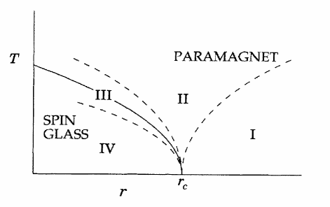
Figure 12: Generic phase diagram (following re:Read95) of the quantum critical behavior for spin glasses. The parameter $r$, which measures the quantum fluctuations, can represent the transverse field for localized spin models or the Fermi energy in metallic spin glasses.

Similarly as in DMFT theories for electronic systems, such infinite range models can be formally reduced to a self-consistent solution of an appropriate quantum impurity problem, as first discussed in the context of quantum spin glasses by Bray and Moore braymoore80. Early work quickly established the phase diagram dobrosavljevic87 of this model, but the dynamics near the quantum critical point proved more difficult to unravel, even when the critical point is approached form the quantum-disordered side. Here, the problem reduces to solving for the dynamics of a single Ising spin in a transverse field, described by an effective Hamiltonian re:Miller93 of the form

$$H=-\frac{1}{2}J^{2}\int\int d\tau d\tau^{\prime}\sigma^{z}(\tau)\chi(\tau-\tau^{\prime})\sigma^{z}(\tau^{\prime})+\Gamma\int d\tau\sigma^{x}(\tau).$$

Physically, the interaction of the considered spin with the spin fluctuations of its environment generates the retarded interaction described by the “memory kernel” $\chi(\tau-\tau^{\prime})$. An appropriate self-consistency condition relates the memory kernel to the disorder-averaged local dynamical susceptibility of the quantum spin

$$\chi(\tau-\tau^{\prime})=\overline{\left\langle T\sigma^{z}(\tau)\sigma^{z}(\tau^{\prime})\right\rangle}.$$

A complete solution of the quantum critical behavior can be obtained, as first established in a pioneering work by Miller and Huse re:Miller93. These authors have set up a diagrammatic perturbation theory for the dynamic susceptibility, showing that the leading loop approximation already captures the exact quantum critical behavior, as the higher order corrections provide only quantitative renormalizations. The dynamical susceptibility takes the general form

$$\chi(\omega_{n})=\chi_{o}+\left(\omega_{n}^{2}+\Delta^{2}\right)^{1/2},$$

where the local static susceptibility $\chi_{o}$ remains finite throughout the critical regime, and the spin excitations exist above a gap

$$\Delta\sim\left(r/\left|\ln r\right|\right)^{1/2}$$

which vanishes as the transition is approached from the paramagnetic side (here $r=\left(\Gamma-\Gamma_{c}\right)/\Gamma_{c}$ measures the distance from the critical point).

• The quantum spin-glass phase and the replicon mode

The validity of this solution was confirmed by a generalization ye93 to the $M$-component rotor model (the Ising model belongs to the same universality class as the $M=2$ rotor model), which can be solved in closed form in the large $M$ limit. This result, which proves to be exact to all orders in the $1/M$ expansion, could be extended even to the spin glass phase, where a full replica symmetric solution was obtained. Most remarkably, the spin excitation spectrum remains gapless ($\Delta=0$) throughout the ordered phase. Such gapless excitations commonly occur in ordered states with broken continuous symmetry, but are generally not expected in classical or quantum models with a discrete symmetry of the order parameter. In glassy phases (at least within mean-field solutions), however, gapless excitations generically arise for both classical and quantum models. Here, they reflect the marginal stability re:Mezard86 found in the presence of replica symmetry breaking, a phenomenon which reflects the high degree of frustration in these systems. The role of the Goldstone mode in this case is played by the so-called “replicon” mode, which describes the collective low energy excitations characterizing the glassy state.

A proper treatment of the low energy excitations in this regime requires special attention to the role of replica symmetry breaking (RSB) in the $T\rightarrow 0$ limit. The original work ye93 suggested that RSB is suppressed at $T=0$, so that the simpler replica symmetric solution can be used at low temperatures. Later work georgesetal01, however, established that the full RSB solution must be considered before taking the $T\rightarrow 0$ limit, and only then can the correct form of the leading low temperature corrections (e.g., the linear $T$-dependence of the specific heat) be obtained.

• Physical content of the mean-field solution

In appropriate path-integral language dobrosavljevic87,ye93, the problem can be shown to reduce to solving a one dimensional classical Ising model with long-range interactions, the form of which must be self-consistently determined. Such classical spin chains with long range interactions in general can be highly nontrivial. Some important examples are the Kondo problem Yuval-Anderson1,Yuval-Anderson2,Yuval-Anderson3, and the dissipative two-level system leggettetal87, both of which map to an Ising chain with $1/\tau^{2}$ interactions. Quantum phase transitions in these problems correspond to the Kosterlitz-Thouless transition found in the Ising chain kosterlitz76prl, the description of which required a sophisticated renormalization-group analysis. Why then is the solution of the quantum Ising spin glass model so simple? The answer was provided in the paper by Ye, Sachdev, and Read ye93, which emphasized that the critical state (and the RSB spin-glass state) does not correspond to the critical point, but rather to the high-temperature phase of the equivalent Ising chain, where a perturbative solution is sufficient. In Kondo language, this state corresponds to the Fermi-liquid solution characterized by a finite Kondo scale, as demonstrated by a quantum Monte-Carlo calculation of Rozenberg and Grempel rozenberg98prl, which also confirmed other predictions of the analytical theory.

From a more general perspective, the possibility of obtaining a simple analytical solution for quantum critical dynamics has a simple origin. It follows from the fact that all corrections to Gaussian (i.e. Landau) theory are irrelevant above the upper critical dimension, as first established by the Hertz-Millis theory hertz,millis for conventional quantum criticality. The mean-field models become exact in the limit of infinite dimensions, hence the Gaussian solution of Refs. re:Miller93,ye93 becomes exact. Leading corrections to mean-field theory for rotor models were examined by an $\varepsilon$-expansion below the upper critical dimension $d_{c}=8$ for the rotor models by Read, Sachdev, and Ye, but these studies found run-away flows, presumably indicating non-perturbative effects that require more sophisticated theoretical tools. Most likely these include Griffiths phase phenomena controlled by the infinite randomness fixed point, as already discussed in Section 3.

• Metallic spin glasses

A particularly interesting role of the low-lying excitations associated with the spin-glass phase is found in metallic spin glasses. Here the quantum fluctuations are provided by the Kondo coupling between the conduction electrons and local moments, and therefore can be tuned by controlling the Fermi energy in the system. The situation is again the simplest for Ising spins where an itinerant version of the rotor model of Sengupta and Georges senguptageorges can be considered, and similar results have obtained for the “spin-density glass” model of Sachdev, Read, and Oppermann sachdevreadopper. The essential new feature in these models is the presence of itinerant electrons which, as in the Hertz-Millis approach hertz,millis, have to be formally integrated out before an effective order-parameter theory can be obtained. This is justified provided that the quasiparticles remain well defined at the quantum critical point, i.e. that the quasiparticle weight $Z\sim T_{K}$ remains finite and the Kondo effect remains operative. The validity of these assumptions is by no means obvious, and led to considerable controversy before a detailed quantum Monte Carlo solution of the model became available rozenberg99prb, confirming the proposed scenario.

Under these assumptions, the theory can again be solved in closed form, and we only quote the principal results. Physically, the essential modification is that the presence of itinerant electrons now induces Landau damping, which creates dissipation for the collective mode. As a result, the dynamics is modified, and the local dynamic susceptibility now takes the following form

$$\chi(\omega_{n})=\chi_{o}+\left(\left|\omega_{n}\right|+\omega^{\ast}\right)^{1/2}.$$ (72)

The dynamics is characterized by the crossover scale $\omega^{\ast}\sim r$ ($r$ measures the distance to the transition) which defines a crossover temperature $T^{\ast}\sim\omega^{\ast}$ separating the Fermi liquid regime (at $T\ll T^{\ast}$) from the quantum critical regime (at $T\gg T^{\ast}$). At the critical point $\chi(\omega_{n})=\chi_{o}+\left|\omega_{n}\right|^{1/2}$, leading to non-Fermi liquid behavior of all physical quantities, which acquire a leading low-temperature correction of the $T^{3/2}$ form. This is a rather mild violation of Fermi liquid theory, since both the static spin susceptibility and the specific heat coefficient remain finite at the QCP. A more interesting feature, which is specific to glassy systems, is the persistence of such quantum critical non-Fermi-liquid behavior throughout the metallic glass phase, reflecting the role of the replicon mode.

Spin-liquid behavior, destruction of the Kondo effect by bosonic dissipation, and fractionalization

• Quantum Heisenberg spin glass and the spin-liquid solution

Quantum spin glass behavior proves to be much more interesting in the case of Heisenberg spins, where the Berry phase term Fradkin plays a highly nontrivial role, completely changing the dynamics even within the paramagnetic phase. While the existence of a finite temperature spin-glass transition was established even in early work braymoore80, solving for the details of the dynamics proved difficult until the remarkable work of Sachdev and Ye sachdevye. By a clever use of large-$N$ methods, these authors identified a striking spin-liquid solution within the paramagnetic phase. In contrast to the nonsingular behavior of Ising or rotor quantum spin glasses, the dynamical susceptibility now displays a logarithmic singularity at low frequency. On the real axis it takes the form

$$\chi(\omega)\sim\ln(1/\left|\omega\right|)+i\frac{\pi}{2}\mathrm{sgn}(\omega).$$

A notable feature of this solution is that it is precisely of the form postulated for “marginal Fermi liquid” phenomenology mfl of doped cuprates. The specific heat is also found to assume a singular form $C\sim\sqrt{T}$, which was shown georgesetal01 to reflect a nonzero extensive entropy if the spin liquid solution is extrapolated to $T=0$. Of course, the spin-liquid solution becomes unstable at a finite ordering temperature, and the broken symmetry state has to be examined to discuss the low temperature properties of the model.

Subsequent work georgesetal01 demonstrated that this mean-field solution remains valid for all finite $N$ and generalized the solution to the spin-glass (ordered) phase. A closed set of equations describing the low temperature thermodynamics in the spin glass phase was obtained, which was very recently re-examined in detail rozenberg04prl to reveal fairly complicated behavior.

• Metallic Heisenberg spin glasses and fractionalization

Even more interesting is the fate of this spin liquid solution in itinerant systems, where an additional Kondo coupling is added between the local moments and the conduction electrons. The mean-field approach can be extended to this interesting situation by examining a Kondo-Heisenberg spin glass model burdinetal with the Hamiltonian

$$H_{KH}=-t\sum_{\langle ij\rangle\sigma}(c_{i\sigma}^{\dagger}c_{j\sigma}^{\phantom{\dagger}}+\mbox{H. c.})+J_{K}\sum_{i}\mathbf{S}_{i}\cdot\mathbf{s}_{i}+\sum_{\langle ij\rangle}J_{ij}\mathbf{S}_{i}\cdot\mathbf{S}_{j}.$$ (73)

In the regime where the scale of the RKKY interaction $J=\left\langle J_{ij}^{2}\right\rangle^{1/2}$ is small compared to the Kondo coupling $J_{K}$, one expects Kondo screening to result in standard Fermi liquid behavior. In the opposite limit, however, the spin fluctuations associated with the retarded RKKY interactions may be able to adversely affect the Kondo screening, and novel metallic behavior could emerge. This intriguing possibility can be precisely investigated in the mean-field (infinite range) limit, where the problem reduces to a single-impurity action of the form burdinetal

$$S_{eff}^{KH} =\sum_{\sigma}\int_{0}^{\beta}d\tau c_{\sigma}^{\dagger}\left(\tau\right)\left(\partial_{\tau}-\mu+v_{j}\right)c_{\sigma}^{\phantom{\dagger}}\left(\tau\right)$$

$$-t^{2}\sum_{\sigma}\int_{0}^{\beta}d\tau\int_{0}^{\beta}d\tau^{\prime}c_{\sigma}^{\dagger}(\tau)G_{c}(\tau-\tau^{\prime})c_{\sigma}^{\phantom{\dagger}}(\tau^{\prime})$$

$$+J_{K}\int_{0}^{\beta}d\tau\mathbf{S}(\tau)\cdot\mathbf{s}(\tau)$$

$$-\frac{J^{2}}{2}\int_{0}^{\beta}d\tau\int_{0}^{\beta}d\tau^{\prime}\chi(\tau-\tau^{\prime})\mathbf{S}(\tau)\cdot\mathbf{S}(\tau^{\prime}).$$ (74)

Such a single-impurity action (74) describes the so-called Bose-Fermi Kondo (BFK) impurity model qimiao96prl,sengupta,zhusi02,zaranddemler02 where, in addition to the coupling to the fermionic bath of conduction electrons, the Kondo spin also interacts with a bosonic bath of spin fluctuations, with local spectral density $\chi\left(\omega_{n}\right)$. Because the same BFK model also appears in “extended” DMFT theories qimiao00prb of quantum criticality in clean systems qimiao96prl,sengupta,sietal,zhusi02,zaranddemler02, its properties have been studied in detail and are by now well understood.

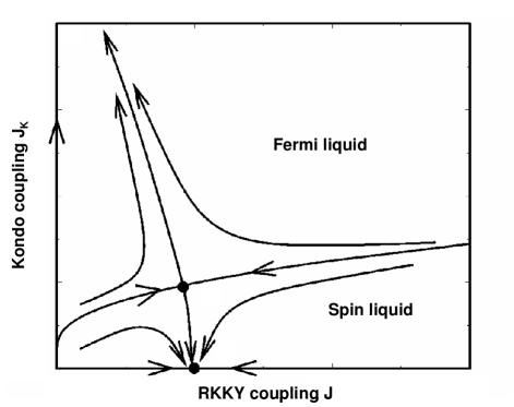
Figure 13: Phase diagram of the Bose-Fermi Kondo model in the presence of a sub-Ohmic bosonic bath qimiao96prl,sengupta,zhusi02,zaranddemler02. Kondo screening is destroyed for sufficiently large dissipation (RKKY coupling to spin fluctuations).

In the absence of the RKKY coupling ($J=0$), the ground state of the impurity is a Kondo singlet for any value of $J_{K}\neq 0$. By contrast, when $J>0$, the dissipation induced by the bosonic bath tends to destabilize the Kondo effect. For a bosonic bath of “Ohmic” form ($\chi\left(\omega_{n}\right)=\chi_{o}-C\left|\omega_{n}\right|$), this effect only leads to a finite decrease of the Kondo temperature, but the Fermi liquid behavior persists. In contrast, for “sub-Ohmic” dissipation ($\chi\left(\omega_{n}\right)=\chi_{o}-C\left|\omega_{n}\right|^{1-\epsilon}$ with $\epsilon>0)$ two different phases exist, and for sufficiently large RKKY coupling the Kondo effect is destroyed. The two regimes are separated by a quantum phase transition (see Fig. 13).

Of course, in the considered Kondo lattice model with additional RKKY interactions, the form of the bosonic bath $\chi\left(\omega_{n}\right)$ is self-consistently determined and can take different forms as the RKKY coupling $J$ is increased. The model was analytically solved within a large $N$ approach by Burdin et al. burdinetal, who calculated the evolution of the Fermi liquid coherence scale $T^{\ast}$ and the corresponding quasiparticle weight $Z$ in the presence of RKKY interactions. Within the paramagnetic phase both $T^{\ast}(J)$ and $Z(J)$ are found to decrease with $J$ until the Kondo effect (and thus the Fermi liquid) is destroyed at $J=J_{c}\approx 10T_{K}^{o}$ (here $T_{K}^{o}$ is the $J=0$ Kondo temperature), where both scales vanish burdinetal,tanaskovic-2005-95. At $T>T^{\ast}(J)$ (and of course at any temperature for $J>J_{c}$) the spins effectively decouple from conduction electrons and spin liquid behavior, essentially identical to that of the insulating model, is established. Thus, sufficiently strong and frustrating RKKY interactions are able to suppress Fermi liquid behavior, and marginal Fermi liquid behavior emerges in a metallic system. This phenomenon, corresponding to spin-charge separation resulting from the destruction of the Kondo effect, is sometimes called “fractionalization” colemanandrei,kaganetal92,demleretal02,senthiletal,senthiletal2. Such behavior has often been advocated as an appealing scenario for exotic phases of strongly correlated electrons, but with the exception of the described model, there are very few well established results and model calculations to support its validity. Finally, we should mention related work parcolletgeorges on doped Mott insulators with random exchanges, with many similarities with the above picture.

We should note, however, that this exotic solution is valid only within the paramagnetic phase, which is generally expected to become unstable to magnetic (spin glass) ordering at sufficiently low temperatures. Since fractionalization emerges only for sufficiently large RKKY coupling (in the large $N$ model $J_{c}\approx 10T_{K}^{o}$), while in general one expects magnetic ordering to take place already at $J\sim T_{K}^{o}$ (according to the famous Doniach criterion Doniach), one expects burdinetal the system to magnetically order much before the Kondo temperature vanishes. If this is true, then one expects the quantum critical behavior to be very similar to metallic Ising spin glasses, i.e., to assume the conventional Hertz-Millis form, at least for the mean-field spin glass models we discussed here. The precise relevance of this paramagnetic spin liquid solution thus remains unclear, at least for systems with weak or no disorder in the conduction band.

• Fractionalized two-fluid behavior of electronic Griffiths phases

The situation seems more promising in the presence of sufficient amounts of disorder, where the electronic Griffiths phase forms. Here the disorder generates a very broad distribution of local Kondo temperatures, making the system much more sensitive to RKKY interactions. This mechanism has recently been studied within an extended DMFT approach tanaskovic-2005-95, which is able to incorporate both the formation of the Griffiths phase and the effects of frustrating RKKY interactions leading to spin-glass dynamics. At the local impurity level, the problem is still reduced to the Bose-Fermi Kondo model, but the presence of conduction electron disorder qualitatively modifies the self-consistency conditions determining the form of $\chi\left(\omega_{n}\right)$.

To obtain a sufficient condition for decoupling, we examine the stability of the Fermi liquid solution, by considering the limit of infinitesimal RKKY interactions. To leading order we replace

$$\chi(\omega_{n})\longrightarrow\chi_{o}\left(\omega_{n}\right)\equiv\chi(\omega_{n};J=0),$$

and the calculation reduces to the “bare model” of Ref. tanaskovic-2005-95. In this case, $P\left(T_{K}\right)\sim T_{K}^{\alpha-1}$, where $\alpha\sim 1/W^{2}$, and

$$\chi_{0}\left(\omega_{n}\right)\sim\int dT_{K}P\left(T_{K}\right)\chi\left(\omega_{n},T_{K}\right)\sim\chi_{0}\left(0\right)-C_{0}\left|\omega_{n}\right|^{1-\epsilon},$$ (75)

where $\epsilon=2-\alpha$. Thus, for sufficiently strong disorder (i.e. within the electronic Griffiths phase), even the “bare” bosonic bath is sufficiently singular to generate decoupling. The critical value of $W$ will be modified by self-consistency, but it is clear that decoupling will occur for sufficiently large disorder.

Once decoupling is present, the system is best viewed as composed of two fluids, one made up of a fraction $n$ of decoupled spins, and the other of a fraction $(1-n)$ of Kondo screened spins. The self-consistent $\chi\left(\omega_{n}\right)$ acquires contributions from both fluids

$$\chi\left(\omega_{n}\right)=n\chi_{dc}\left(\omega_{n}\right)+\left(1-n\right)\chi_{s}\left(\omega_{n}\right).$$ (76)

A careful analysis tanaskovic-2005-95 shows that, for a bath characterized by an exponent $\epsilon$

$$\chi_{dc}\left(\omega_{n}\right) \sim\chi_{dc}\left(0\right)-C\left|\omega_{n}\right|^{1-\left(2-\epsilon\right)};$$ (77)

$$\chi_{s}\left(\omega_{n}\right) \sim\chi_{s}\left(0\right)-C^{\prime}\left|\omega_{n}\right|^{1-\left(2-\epsilon-1/\nu\right)},$$ (78)

where $\nu=\nu\left(\epsilon\right)$ is a critical exponent governing how the Kondo scale vanishes at the quantum critical point of the Bose-Fermi model. Since $\nu>0$, the contribution of the decoupled fluid is more singular and dominates at lower frequencies. Self-consistency then yields $\epsilon=1$, as in the familiar spin liquid state of Sachdev and Ye sachdevye. For $\epsilon=1$, the local susceptibility is logarithmically divergent (both in $\omega_{n}$ and $T$). This does not necessarily mean that the bulk susceptibility, which is the experimentally relevant quantity, behaves in the same manner parcolletgeorges. More work remains to be done to determine the precise low temperature form of this and other physical quantities and to assert the relevance of this mechanism for specific materials.

As in the case where conduction electron disorder is absent, the spin liquid state is unstable towards spin-glass ordering at sufficiently low temperatures. However, numerical estimates for the Griffiths phase model tanaskovic-2005-95 suggest a surprisingly wide temperature window where the marginal behavior should persist above the ordering temperature. Fig. 14 represents the predicted phase diagram of this model. For weak disorder the system is in the Fermi liquid phase, while for $W>W_{c}$ the marginal Fermi liquid phase emerges. The crossover temperature (dashed line) delimiting this regime can be estimated from the frequency up to which the logarithmic behavior of the local dynamical susceptibility $\chi(i\omega)$ is observed. The spin glass phase, obtained from Eq. (70), appears only at the lowest temperatures, well below the marginal Fermi liquid boundary. Interestingly, recent experiments dougetal have indeed found evidence of dynamical spin freezing in the milliKelvin temperature range for the same Kondo alloys that display normal phase non-Fermi-liquid behavior in a much broader temperature window.

Figure 14: Phase diagram of the electronic Griffiths phase model with RKKY interactions tanaskovic-2005-95. The inset shows the fraction of decoupled spins as a function of the disorder strength $W$.

The two-fluid phenomenology of the disordered Kondo lattice we have described above is very reminiscent of earlier work on the clean Kondo lattice, where the conduction electrons effectively decouple from the local moments, the latter forming a spin liquid state colemanandrei,kaganetal92,demleretal02,senthiletal,senthiletal2. The major difference between the results presented in this Section and these other cases is that here local spatial disorder fluctuations lead to an inhomogeneous coexistence of the two fluids, as each site decouples or not from the conduction electrons depending on its local properties. The discussed mean-field models should be considered as merely the first examples of this fascinating physics. The specific features of the spin liquid behavior that was obtained from these models may very well prove to be too restrictive and perhaps even inaccurate. For example, the specific heat enhancements may well be overestimated, reflecting the residual $T=0$ entropy of the mean-field models. Nevertheless, the physics of Kondo screening being destroyed by the interplay of disorder and RKKY interactions will almost certainly play a central role in determining the properties of many non-Fermi-liquid systems, and clearly needs to be investigated in more detail in the future.

2 Electron glass

Another aspect of disordered interacting electrons poses a fundamental problem. Very generally, Coulomb repulsion favors a uniform electronic density, while disorder favors local density fluctuations. When these two effects are comparable in magnitude, one can expect many different low energy electronic configurations, i.e. the emergence of many metastable states. Similarly as in other “frustrated” systems with disorder, such as spin glasses, these processes can be expected to lead to glassy behavior of the electrons, and the associated anomalously slow relaxational dynamics. Indeed, both theoretical eglass1,eglass2 and experimental films22,films23,bogdanovich-prl02,JJPRL02 work has found evidence of such behavior deep on the insulating side of the transition. However, at present very little is known as to the precise role of such processes in the critical region. Nevertheless, it is plausible that the glassy freezing of the electrons must be important, since the associated slow relaxation clearly will reduce the mobility of the electrons. From this point of view, the glassy freezing of electrons may be considered, in addition to the Anderson and the Mott mechanism, as a third fundamental process associated with electron localization. Interest in understanding the glassy aspects of electron dynamics has experienced a genuine renaissance in the last few years, primarily due to experimental advances. Emergence of many metastable states, slow relaxation and incoherent transport have been observed in a number of strongly correlated electronic systems. These included transition metal oxides such as high T_c materials, manganites, and ruthenates. Similar features have recently been reported in two-dimensional electron gases and even three-dimensional doped semiconductors such as Si:P.

• Infinite-dimensional model of an electron glass

The interplay of the electron-electron interactions and disorder is particularly evident deep on the insulating side of the metal-insulator transition (MIT). Here, both experimental re:Massey96 and theoretical studies re:Efros75 have demonstrated that they can lead to the formation of a soft “Coulomb gap”, a phenomenon that is believed to be related to the glassy behavior films22,films23,bogdanovich-prl02,JJPRL02 of the electrons. Such glassy freezing has long been suspected re:Belitz95 to be of importance, but more recent theoretical work gang4me,Sudip has suggested that it may even dominate the MIT behavior in certain low carrier density systems. The classic work of Efros and Shklovskii re:Efros75 has clarified some basic aspects of this behavior, but a number of key questions have remain unanswered.

As a simplest example pastor-prl99 displaying glassy behavior of electrons, we focus on a simple lattice model of spinless electrons with nearest neighbor repulsion $V$ in presence of random site energies $\varepsilon_{i}$ and inter-site hopping $t$, as given by the Hamiltonian

$$H=\sum_{<ij>}(-t_{ij}+\varepsilon_{i}\delta_{ij})c^{\dagger}_{i}c_{j}+V\sum_{<ij>}c^{\dagger}_{i}c_{i}c^{\dagger}_{j}c_{j}.$$ (79)

This model can be solved in a properly defined limit of large coordination number georgesrmp, where an extended dynamical mean-field theory (EDMFT) formulation becomes exact. We concentrate on the situation where the disorder (or more generally frustration) is large enough to suppress any uniform ordering. We then rescale both the hopping elements and the interaction amplitudes as $t_{ij}\rightarrow t_{ij}/\sqrt{z}$;    $V_{ij}\rightarrow V_{ij}/\sqrt{z}$. As we will see shortly, the required fluctuations then survive even in the $z\rightarrow\infty$ limit, allowing for the existence of the glassy phase. Within this model:

$\star$

The universal form of the Coulomb gap re:Efros75 proves to be a direct consequence of glassy freezing.

$\star$

The glass phase is identified through the emergence of an extensive number of metastable states, which in our formulation is manifested as a replica symmetry breaking instability re:Mezard86.

$\star$

As a consequence of this ergodicity breaking re:Mezard86, the zero-field cooled compressibility is found to vanish at T=0, suggesting the absence of screening re:Efros75 in disordered insulators.

$\star$

The quantum fluctuations can melt this glass even at $T=0$, but the relevant energy scale is set by the electronic mobility and is therefore a nontrivial function of disorder.

We should stress that although this model allows us to examine the interplay of glassy ordering and quantum fluctuations due to itinerant electrons, it is too simple to describe the effects of Anderson localization. These effects require extensions to lattices with finite coordination and will be discussed in the next section.

For simplicity, we focus on a Bethe lattice at half filling and examine the $z\rightarrow\infty$ limit. This strategy automatically introduces the correct order parameters and after standard manipulations dk-prb94 the problem reduces to a self-consistently defined single site problem, as defined by an the effective action of the form

$$S_{eff}(i)=\sum_{a}\int_{o}^{\beta}\int_{o}^{\beta}d\tau d\tau^{\prime}\;[c^{\dagger a}_{i}(\tau)(\delta(\tau-\tau^{\prime})\partial_{\tau}+\varepsilon_{i}+t^{2}G(\tau,\tau^{\prime}))c^{a}_{i}(\tau^{\prime})$$

$$+\frac{1}{2}V^{2}\delta n_{i}^{a}(\tau)\chi(\tau,\tau^{\prime})\delta n_{i}^{a}(\tau^{\prime})]+\frac{1}{2}V^{2}\sum_{a\neq b}\int_{o}^{\beta}\int_{o}^{\beta}d\tau d\tau^{\prime}\;\delta n_{i}^{a}(\tau)\;q_{ab}\;\delta n_{i}^{b}(\tau^{\prime}).$$ (80)

Here, we have used functional integration over replicated Grassmann fields dk-prb94 $c_{i}^{a}(\tau)$ that represent electrons on site $i$ and replica index $a$, and the random site energies $\varepsilon_{i}$ are distributed according to a given probability distribution $P(\varepsilon_{i})$. The operators $\delta n_{i}^{a}(\tau)=(c^{\dagger a}_{i}(\tau)c_{i}^{a}(\tau)-1/2)$ represent the density fluctuations from half filling. The order parameters $G(\tau-\tau^{\prime})$, $\chi(\tau-\tau^{\prime})$ and $q_{ab}$ satisfy the following set of self-consistency conditions

$$G(\tau-\tau^{\prime})=\int d\varepsilon_{i}P(\varepsilon_{i})<c^{\dagger a}_{i}(\tau)c_{i}^{a}(\tau^{\prime})>_{eff},$$ (81)

$$\chi(\tau-\tau^{\prime})=\int d\varepsilon_{i}P(\varepsilon_{i})<\delta n^{\dagger a}_{i}(\tau)\delta n_{i}^{a}(\tau^{\prime})>_{eff},$$ (82)

$$q_{ab}=\int d\varepsilon_{i}P(\varepsilon_{i})<\delta n^{\dagger a}_{i}(\tau)\delta n_{i}^{b}(\tau^{\prime})>_{eff}.$$ (83)

• Order parameters

In these equations, the averages are taken with respect to the effective action of Eq. (80). Physically, the “hybridization function” $t^{2}G(\tau-\tau^{\prime})$ represents the single-particle electronic spectrum of the environment, as seen by an electron on site $i$. In particular, its imaginary part at zero frequency can be interpreted dk-prb94 as the inverse lifetime of the local electron and as such remains finite as long as the system is metallic. We recall dk-prb94 that for $V=0$ these equations reduce to the familiar CPA description of disordered electrons, which is exact for $z=\infty$. The second quantity $\chi(\tau-\tau^{\prime})$ represents an (interaction-induced) mode-coupling term that reflects the retarded response of the density fluctuations of the environment. Note that very similar objects appear in the well-known mode-coupling theories of the glass transition in dense liquids re:Cummins94. Finally the quantity $q_{ab}$ $(a\neq b)$ is nothing but the familiar Edwards-Anderson order parameter $q_{EA}$. Its nonzero value indicates that the time averaged electronic density is spatially non-uniform.

• Equivalent Infinite Range model

From a technical point of view, a RSB analysis is typically carried out by focusing on a free energy expressed as a functional of the order parameters. In our Bethe lattice approach, one directly obtains the self-consistency conditions from appropriate recursion relations dk-prb94, without invoking a free energy functional. However, we have found it useful to map our $z=\infty$ model to another infinite range model, which has exactly the same set of order parameters and self-consistency conditions, but for which an appropriate free energy functional can easily be determined. The relevant model is still given Eq. (79), but this time with random hopping elements $t_{ij}$ and random nearest-neighbor interaction $V_{ij}$, having zero mean and variances $t^{2}$, and $V^{2}$, respectively. For this model, standard manipulations dk-prb94 result in the following free energy functional

$$F[G,\chi,q_{ab}]= - \frac{1}{2}\sum_{a}\int_{o}^{\beta}\int_{o}^{\beta}d\tau d\tau^{\prime}\;[t^{2}G^{2}(\tau,\tau^{\prime})+V^{2}\chi^{2}(\tau,\tau^{\prime})]-\frac{1}{2}\sum_{a\neq b}(\beta V)^{2}q^{2}_{ab}$$ (84)

$$- \ln\left[\int d\varepsilon_{i}P(\varepsilon_{i})\int Dc^{\dagger a}_{i}Dc^{a}_{i}\exp\left\{-S_{eff}(i)\right\}\right],$$

with $S_{eff}(i)$ given by Eq. (80). The self-consistency conditions, Eqs. (81-83) then follow from

$$0=\delta F/\delta G(\tau,\tau^{\prime});\;0=\delta F/\delta\chi(\tau,\tau^{\prime});\;0=\delta F/\delta q_{ab}.$$ (85)

We stress that Eqs. (81-83) have been derived for the model with uniform hopping elements $t_{ij}$ and interaction amplitudes $V_{ij}$, in the $z\rightarrow\infty$ limit, but the same equations hold for an infinite range model where these parameters are random variables.

• The glass transition

In our electronic model, the random site energies $\varepsilon_{i}$ play a role of static random fields. As a result, in the presence of disorder, the Edwards-Anderson parameter $q_{EA}$ remains nonzero for any temperature, and thus cannot serve as an order parameter. To identify the glass transition, we search for a replica symmetry breaking (RSB) instability, following standard methods re:AT,re:Mezard92. We define $\delta q_{ab}=q_{ab}-q$, and expand the free energy functional of Eq. (84) around the replica symmetric solution. The resulting quadratic form (Hessian matrix) has the matrix elements given by

$$\frac{\partial^{2}F}{\partial q_{ab}\partial q_{cd}} = (\beta V)^{2}\delta_{ac}\delta_{bd}+[<\delta n_{a}(\tau_{1})\delta n_{b}(\tau_{2})>_{RS}<\delta n_{c}(\tau_{3})\delta n_{d}(\tau_{4})>_{RS}$$

$$- V^{4}\int_{0}^{\beta}\int_{0}^{\beta}\int_{0}^{\beta}\int_{0}^{\beta}d\tau_{1}d\tau_{2}d\tau_{3}d\tau_{4}[<\delta n_{a}(\tau_{1})\delta n_{b}(\tau_{2})\delta n_{c}(\tau_{3})\delta n_{d}(\tau_{4})>_{RS}],$$

where the expectation values are calculated in the RS solution. Using standard manipulations re:AT, and after lengthy algebra, we finally arrive at the desired RSB stability criterion that takes the form

$$1=V^{2}\left[\left(\chi_{loc}(\varepsilon_{i})\right]^{2}\right]_{dis}.$$ (87)

Here, $[...]_{dis}$ indicates the average over disorder and $\chi_{loc}(\varepsilon_{i})$ is the local compressibility, that can be expressed as

$$\chi_{loc}(\varepsilon_{i})=\frac{\partial}{\partial\varepsilon_{i}}\frac{1}{\beta}\int_{o}^{\beta}d\tau<\delta n_{i}(\tau)>,$$ (88)

and which is evaluated by carrying out quantum averages for a fixed realization of disorder. The relevant expectation values have to be carried with respect to the full local effective action $S_{eff}(i)$ of Eq. (2), evaluated in the RS theory. In general, the required computations cannot be carried out in closed form, primarily due to the unknown “memory kernel” $\chi(\tau-\tau^{\prime})$. However, as we will see, the algebra simplifies in several limits, where explicit expressions can be obtained.

• Classical electron glass

In the classical $(t=0)$ limit, the problem can be easily solved in closed form. We first focus on the replica symmetric (RS) solution and set $q_{ab}=q$ for all replica pairs. The corresponding equation reads

$$q=\frac{1}{4}\int_{-\infty}^{+\infty}\frac{dx}{\sqrt{\pi}}e^{-x^{2}/2}\tanh^{2}\left[\frac{1}{2}x\left((\beta V)^{2}q+(\beta W)^{2}\right)^{1/2}\right],$$ (89)

where we have considered a Gaussian distribution of random site energies of variance $W^{2}$. Note that the interactions introduce an effective, enhanced disorder strength

$$W_{eff}=\sqrt{W^{2}+V^{2}q},$$ (90)

since the frozen-in density fluctuations introduce an added component to the random potential seen by the electrons. As expected, $q\neq 0$ for any temperature when $W\neq 0$. If the interaction strength is appreciable as compared to disorder, we thus expect the resistivity to display an appreciable increase at low temperatures. We emphasize that this mechanism is different from Anderson localization, which is going to be discussed in the next section, but which also gives rise to a resistivity increase at low temperatures.

Next, we examine the instability to glassy ordering. In the classical ($t=0$) limit Eq. (87) reduces to

$$1=\frac{1}{16}(\beta V)^{2}\int_{-\infty}^{+\infty}\frac{dx}{\sqrt{\pi}}e^{-x^{2}/2}\cosh^{-4}\left[\frac{1}{2}x\beta W_{eff}(q)\right],$$ (91)

with $W_{eff}(q)$ given by Eq.(90). The resulting RSB instability line separates a low temperature glassy phase from a high temperature “bad metal” phase. At large disorder, these expressions simplify and we find

$$T_{G}\approx\frac{1}{6\sqrt{2\pi}}\frac{V^{2}}{W},\;W\rightarrow\infty.$$ (92)

We conclude that $T_{G}$ decreases at large disorder. This is to be expected, since in this limit the electrons drop into the lowest potential minima of the random potential. This defines a unique ground state, suppressing the frustration associated with the glassy ordering and thus reducing the glassy phase. It is important to note that for the well known de Almeida-Thouless (AT) line $T_{RSB}$ decreases exponentially in the strong field limit. In contrast, we find that in our case, $T_{G}\sim 1/W$ decreases only slowly in the strong disorder limit. This is important, since the glassy phase is expected to be most relevant for disorder strengths sufficient to suppress uniform ordering. At the same time, glassy behavior will only be observable if the associated glass transition temperature remains appreciable.

• The glassy phase

To understand this behavior, we investigate the structure of the low-temperature glass phase. Consider the single-particle density of states at T=0, which in the classical limit can be expressed as

$$\overline{\rho}(\varepsilon,t=0)=\frac{1}{N}\sum_{i}\delta(\varepsilon-\varepsilon^{R}_{i}),$$ (93)

where $\varepsilon_{i}^{R}\equiv\varepsilon_{i}+\sum V_{ij}n_{j}$ are the renormalized site energies. In the thermodynamic limit, this quantity is nothing but the probability distribution $P_{R}(\varepsilon^{R}_{i})$. It is analogous to the “local field distribution” in the spin-glass models and can be easily shown to reduce to a simple Gaussian distribution in the RS theory, establishing the absence of any gap for $T>T_{G}$. Obtaining explicit results from a replica calculation in the glass phase is more difficult, but useful insight can be achieved by using standard simulation methods re:Palmer79,re:Pazmandi99 on our equivalent infinite-range model; some typical results are shown in Fig. 15.

Figure 15: Single particle density of states in the classical ($t=0$) limit at $T=0$, as a function of disorder strength. Results are shown from a simulation on $N=200$ site system, for $W/V=0.5$ (thin line) and $W/V=1.0$ (full line). Note that the low energy form of the gap takes a universal form, independent of the disorder strength $W$. The dashed line follows Eq. (94).

We find that as a result of glassy freezing, a pseudo-gap emerges in the single-particle density of states, reminiscent of the Coulomb gap of Efros and Shklovskii (ES) re:Efros75. The low energy form of this gap appears universal,

$$\rho(\varepsilon)\approx C\varepsilon^{\alpha}/V^{2},\;\mathrm{for}\;\varepsilon<E_{g};\;\;\;C=\alpha=1,$$ (94)

independent of the disorder strength $W$, again in striking analogy with the predictions of ES. To establish this result, we have used stability arguments very similar to those developed for spin-glass (SG) models re:Pazmandi99, demonstrating that the form of Eq. (94) represents an exact upper bound for $\rho(\varepsilon)$. For infinite-ranged SG models, as in our case, this bound appears to be saturated, leading to universal behavior. Such universality is often associated with a critical, self-organized state of the system. Recent work re:Pazmandi99 finds strong numerical evidence of such criticality for SG models; we believe that the universal gap form in our case has the same origin. Furthermore, assuming that the universal form of Eq. (94) is obeyed immediately allows for an estimate of $T_{G}(W)$. Using Eq. (87) to estimate the gap size for large disorder gives $T_{G}\sim E_{g}\sim V^{2}/W$, in agreement with Eq. (92).

The ergodicity breaking associated with the glassy freezing has important consequences for our model. Again, using the close similarity of our classical infinite range model to standard SG models re:Mezard86, it is not difficult to see that the zero-field cooled (ZFC) compressibility vanishes at $T=0$, in contrast to the field-cooled one, which remains finite. Essentially, if the chemical potential is modified after the system is cooled to $T=0$, the system immediately falls out of equilibrium and displays hysteretic behavior re:Pazmandi99 with vanishing typical compressibility. If this behavior persists in finite dimensions and for more realistic Coulomb interactions, it could explain the absence of screening in disordered insulators.

• Arbitrary lattices and finite coordination: mean-field glassy phase of the random-field Ising model

The simplest theories of glassy freezing re:Mezard86 are obtained by examining models with random inter-site interactions. In the case of disordered electronic systems, the interactions are not random, but glassiness still emerges due to frustration introduced by the competition of the interactions and disorder. As we have seen for the Bethe lattice pastor-prl99, random interactions are generated by renormalization effects, so that standard DMFT approaches can still be used. However, one would like to develop systematic approaches for arbitrary lattices and in finite coordination. These issues already appear on the classical level, where our model reduces to the random-field Ising model (RFIM) re:Nattermann97. To investigate the glassy behavior of the RFIM horbach02, a systematic approach that can incorporate short-range fluctuation corrections to the standard Bragg-Williams theory is the method of Plefka re:Plefka and Georges et al. Georges90. This work has shown that: (i) corrections to even the lowest nontrivial order immediately result in the appearance of a glassy phase for sufficiently strong randomness; (ii) this low-order treatment is sufficient in the joint limit of large coordination and strong disorder; (iii) the structure of the resulting glassy phase is characterized by universal hysteresis and avalanche behavior emerging from the self-organized criticality of the ordered state.

• Long-range Coulomb interactions and the Efros-Shklovskii gap

So far we focused on the limit of large coordination, where the EDMFT approximation is essentially exact and the resulting electron glass phase shows many similarities to the standard Parisi theory of spin glasses re:Mezard86. While it produced many appealing results, this mean-field approach has remained very controversial for short-range spin glasses in finite dimensions; a competing “droplet” theory fisherandhuse86 approach suggested that many of Parisi’s predictions may not survive in physical dimensions $d=2,3$. The situation is more promising in the case of the physically relevant long-ranged Coulomb interaction, where the prediction of the mean-field approach may possibly persist even in low dimensions.

The most interesting test of these ideas relates to the possibility of describing the emergence of the “Coulomb gap” in $d=2,3$ for localized electrons interacting via long-range Coulomb interactions, as first predicted, based on heuristic arguments, a long time ago re:Efros75. Here, the single particle density of states is predicted to assume a powerlaw form $g(\varepsilon)\sim\varepsilon^{\gamma}$, notably with a dimensionality-dependent exponent $\gamma=d-1$.

Conventional mean-field theories typically produce universal dimensionality independent exponents and thus cannot be expected to explain this unfamiliar situation. On the other hand, the EDMFT chitra00prl approach does include the effects of spatial correlations, as the bosonic collective modes describing the “cavity field” are treated at a Gaussian level, similar to the familiar Hertz-Millis theories of quantum criticality hertz,millis. When applied to the case of long-range Coulomb interactions, the corresponding plasmon propagator does reflect chitra00prl both the specific form of the long-range interactions and the dimensionality of the system. When applied to disordered electrons, the replica version of this method produces self-consistency conditions which assume a very similar form as in ordinary Parisi theory or the simple infinite range electron glass model we examined in previous sections. Indeed, recent work has generalized our EDMFT method to the long-range models, where the glassy phase of the generalized Coulomb interactions pankov05prl of the form $V(R)\sim 1/R^{\alpha}$ has been examined in finite dimensions. We will not elaborate of the details of these theories here, but we emphasize that most qualitative features of the resulting glassy phase have been found to share very similar behavior muller04prl as for the infinite-range model of electron glasses, including the corresponding pattern of replica symmetry breaking pankov06prl,pankov07prb. Most remarkably, however, this theory produced pankov05prl an interaction-range and dimensionality dependent Coulomb gap exponent

$$\gamma=(d-\alpha)/\alpha,$$ (95)

in precise agreement with an appropriate generalization of the Efros-Shklovskii argument re:Efros75. This early result was later confirmed pankov07prb by a more detailed low-temperature solution of the same equations deep in the replica-symmetry broken phase, based on a $T=0$ new solution of the Parisi equation due to Pankov pankov06prl.

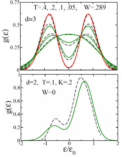
Figure 16: The analytical EDMFT predictions pankov05prl for the single-particle density of states (full lines) are found to be in excellent quantitative agreement with simulation results (dashed lines), with no adjustable parameters. Shown are results for the three dimensional case studied in Ref. re:Sarvestani95, corresponding to $W=1/(2\sqrt{3})$, and temperatures $T=0.4,0.2,0.1,0.05$ (top panel), and the two dimensional model of Ref. efros92prl, corresponding to $W=0$, $T=0.1$, $K=0.2$. Green lines correspond to the fluid pseudogap phase, while the red curve corresponds to $T=0.05$, close to the glass transition temperature.

Another striking result of these theories should be noted. Namely, one finds pankov05prl that the Coulomb pseudogap starts to form around a crossover temperatures $T^{*}\sim T_{C}$ (the Coulomb energy), much above the glass transition temperature $T_{G}\approx 0.05T_{C}$, and in perfect quantitative agreement (Fig. 16 with earlier numerical work clareyu93prl. The EDMFT theory, in fact, demonstrated the following: (1) the universal value of the Efros-Shklovskii exponent $\gamma$ is a direct consequence of the marginal stability of the glassy phase; (2) in contrast, the emergence of a non-universal Coulomb pseudogap in the high temperature regime $T_{G}<T<T^{*}$ is not related to glassy freezing and the breakdown of screening muller04prl,pankov07prb, and is a robust effect found efros92prl even in the absence of disorder. The two mechanisms for pseudogap formation have often been confused clareyu93prl in previous work, leading to incorrect and even misleading interpretations of what determines its form in a given temperature range.

• Quantum melting of the electron glass

Next, we investigate how the glass transition temperature can be depressed by quantum fluctuations introduced by inter-site electron tunneling. For simplicity, we again focus on the simplest infinite-range model of the electron glass. As in other quantum glass problems, quantum fluctuations introduce dynamics in the problem, and the relevant self-consistency equations cannot be solved in closed form for general values of the parameters. In the following, we will see that in the limit of large randomness an exact solution is possible. The main source of difficulty in general quantum glass problems relates to the existence of a self-consistently determined “memory kernel” $\chi(\tau-\tau^{\prime})$ in the local effective action. By the same reasoning as in the classical case, one can also ignore this term since this quantity is also bounded.

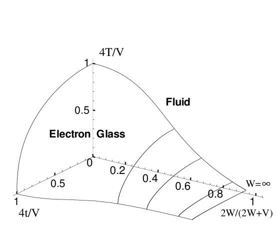
Figure 17: Phase diagram as a function of quantum hopping $t$, temperature $T$ and disorder strength $W$. The glass transition temperature $T_{G}$ decreases only slowly (as $\sim 1/W$) in the strong disorder limit. In contrast, the critical value of the hoping element $t_{G}$ remains finite as $W\rightarrow\infty$

The remaining action is that of noninteracting electrons in the presence of a strong random potential. The resulting local compressibility then takes the form

$$\chi_{loc}(\varepsilon)=\frac{\beta}{4}\int_{-\infty}^{+\infty}d\omega\rho_{\varepsilon}(\omega)\cosh^{-2}(\frac{1}{2}\beta\omega).$$ (96)

Here, $\rho_{\varepsilon}(\omega)$ is the local density of states, which in the considered large $z$ limit is determined by the solution of the CPA equation

$$\rho_{\varepsilon}(\omega)=-\frac{1}{\pi}{\rm Im}G(\omega);\;\;G(\omega)=\int\frac{d\varepsilon P(\varepsilon)}{\omega+i\eta-\varepsilon-t^{2}G(\omega)},$$ (97)

In the limit $W/t>>1$, it reduces to a narrow resonance of width $\Delta=\pi t^{2}P(0)\sim t^{2}/W$

$$\rho_{\varepsilon}(\omega)\approx\frac{1}{\pi}\frac{\Delta}{(\omega-\varepsilon)^{2}+\Delta^{2}}.$$ (98)

The resulting expression for the quantum critical line in the large disorder limit takes the form

$$t_{G}(T=0,W\rightarrow\infty)=V/\sqrt{\pi}.$$ (99)

At first glance, this result is surprising, since it means that a finite value of the Fermi energy is required to melt the electron glass at $T=0$, even in the $W\rightarrow\infty$ limit! This is to be contrasted with the behavior of $T_{G}$ in the classical limit, which according to Eq. (92) was found to decrease as $1/W$ for strong disorder. At first puzzling, the above result in fact has a simple physical meaning. Namely, the small resonance width (or “hybridization energy”) $\Delta\sim t^{2}/W$ can be interpreted anderson58,motand as the characteristic energy scale for the electronic motion. As first pointed out by Anderson anderson58, according to Fermi’s golden rule, the transition rate to a neighboring site is proportional to $\Delta$ and not $t$, and thus becomes extremely small at large disorder. Thus the “size” of quantum fluctuations, which replace the thermal fluctuations at $T=0$, is proportional to $\Delta\sim 1/W$, and thus becomes very small in the large $W$ limit. We can now easily understand the qualitative behavior shown in Eq. (99) by replacing $T_{G}\rightarrow\Delta\sim t_{G}^{2}/W$ in Eq. (92). The leading $W$ dependence cancels out, and we find a finite value for $t_{G}$ in the $W\rightarrow\infty$ limit.

More generally, we can write an expression for the glass transition critical line in the large disorder limit, as a function of $\beta=1/T$ and $t$ in the scaling form

$$1=(V/t)^{2}\phi(\beta t^{2}/W),$$ (100)

with

$$\phi(z)=\frac{1}{4}z^{2}\int_{-\infty}^{+\infty}dx\left[\int_{-\infty}^{+\infty}dy\frac{1}{\pi}\frac{1}{1+(x-y)^{2}}\cosh^{-2}(\frac{1}{2}zy)\right]^{2}.$$ (101)

At finite disorder an exact solution is not possible, but we can make analytical progress motivated by our discussion of the large $W$ limit. Namely, one can imagine evaluating the required local compressibilities in Eq. (88) by a “weak coupling” expansion in powers of the interaction $V$. To leading order, this means evaluating the compressibilities at $V=0$, an approximation which becomes exact for $W$ large. Such an approximation can be tested for other spin glass problems. We have carried out the corresponding computations for the infinite range Ising spin glass model in a transverse field, where the exact critical transverse field is known from numerical studies. We can expect the leading approximation to underestimate the size of the glassy region, i. e. the critical field, since the omitted “memory kernel” introduces long range correlations in time, which make the system more “classical”. Indeed, we find that the leading approximation underestimates the critical field by only about 30%, whereas the next order correction gives an error of less than 5%. Encouraged by these arguments, we use this “weak-coupling” approximation for arbitrary disorder strength $W$. Again, the computation of the compressibility reduces to that of noninteracting electrons in a CPA formulation; the resulting phase diagram is shown in Fig. 17.

• Quantum critical behavior of the electron glass

So far, we have seen how our extended DMFT equations can be simplified for large disorder, allowing an exact computation of the phase boundary in this limit. In our case, this quantum critical line separates a (non-glassy) Fermi liquid phase from a metallic glass phase which, as we will see, features non-Fermi liquid behavior. If one is interested in the details of the dynamics of the electrons near the quantum critical line, the above simplifications do not apply and one is forced to self-consistently calculate the form of the “memory kernel” (local dynamic compressibility) $\chi(\tau-\tau^{\prime})$. Fortunately, this task can be carried out using methods very similar to those developed for DMFT models for metallic spin glasses re:Read95. Formulating such a theory is technically possible because the exact quantum critical behavior is captured when the relevant field theory is examined at the Gaussian level re:Miller93, in the considered limit of large dimensions.

Because of the technical complexity of this calculation, we only report the main results, while the details can be found in Denis. In this paper, the full replica-symmetry broken (RSB) solution was found, both around the quantum critical line and in the glassy phase. In the Fermi liquid phase, the memory kernel was found to take the form

$$V^{2}\chi(\omega_{n})=D(\omega_{n})+\beta q_{{\rm EA}}\delta_{\omega_{n},0},$$

with

$$D(\omega_{n})=-yq_{{\rm EA}}^{2}/V^{4}-\sqrt{|\omega_{n}|+\Delta}.$$

Here, $\Delta$ is a characteristic energy scale that vanishes on the critical line, which also determines the crossover temperature scale separating the Fermi liquid from the quantum-critical regime. In contrast to conventional quantum critical phenomena, but similarly to metallic spin glasses, the “gap” scale $\Delta$ is equal to zero not only on the critical line, but remains zero throughout the entire glassy phase. As a result, the excitations in this region assume a non-Fermi liquid form

$$D(\omega_{n})=-yq_{{\rm EA}}^{2}/V^{4}-\sqrt{|\omega_{n}|}.$$

This behavior reflects the emergence of soft “replicon” modes re:Mezard86 describing in our case low energy charge rearrangements inside the glassy phase. At finite temperatures, electrons undergo inelastic scattering from such collective excitations, leading to a temperature dependence of the resistivity that takes the following non-Fermi liquid form

$$\rho(T)=\rho(o)+AT^{3/2}.$$

Interestingly, very recent experiments bogdanovich-prl02 on two-dimensional electron gases in silicon have revealed precisely such a temperature dependence of the resistivity. This behavior has been observed in what appears to be an intermediate metallic glass phase separating a conventional (Fermi liquid) metal at high carrier density from an insulator at the lowest densities.

Another interesting feature of the predicted quantum critical behavior relates to the disorder dependence of the crossover exponent $\phi$ describing how the gap scale $\Delta\sim\delta r^{\phi}$ vanishes as a function of the distance $\delta r$ from the critical line. Calculations arrachea show that $\phi=2$ in the presence of site energy disorder, which for our model plays the role of a random symmetry breaking field, and $\phi=1$ in its absence. This indicates that site disorder, which is common in disordered electronic systems, produces a particularly large quantum critical region, which could be the origin of the large dephasing observed in many materials near the metal-insulator transition.

• Glassy behavior near the Mott-Anderson transition

As we have seen, the stability of the glassy phase is crucially determined by the electronic mobility at $T=0$. More precisely, we have shown that the relevant energy scale that determines the size of quantum fluctuations introduced by the electrons is given by the local “resonance width” $\Delta$. It is important to recall that precisely this quantity may be considered anderson58 as an order parameter for Anderson localization of noninteracting electrons. Recent work motand,london demonstrated that the typical value of this quantity plays the same role even at a Mott-Anderson transition. We thus expect $\Delta$ to generally vanish in the insulating state. As a result, we expect the stability of the glassy phase to be strongly affected by Anderson localization effects, as we will explicitly demonstrate in the next section.

On physical grounds, one expects the quantum fluctuations pastor-prl99 associated with mobile electrons  to suppress glassy ordering, but their precise effects remain to be elucidated. Note that even the amplitude of such quantum fluctuations must be a singular function of the distance to the MIT, since they are dynamically determined by processes that control the electronic mobility.

To clarify the situation, the following basic questions need to be addressed: (1) Does the MIT coincide with the onset of glassy behavior? (2) How do different physical processes that can localize electrons  affect the stability of the glass phase? In the following, we provide simple and physically transparent  answers to both questions. We find that: (a) Glassy behavior generally emerges before the electrons localize; (b) Anderson localization anderson58 enhances the stability of the glassy phase, while Mott localization mott-book90 tends to suppress it.

In order to be able to examine both the effects of Anderson and Mott localization, we concentrate on extended Hubbard models given by the Hamiltonian

$$H=\sum_{ij\sigma}(-t_{ij}+\varepsilon_{i}\delta_{ij})c_{i,\sigma}^{\dagger}c_{j,\sigma}+U\sum_{i}n_{i\uparrow}n_{i\downarrow}+\sum_{ij}V_{ij}\delta n_{i}\delta n_{j}.$$

Here, $\delta n_{i}=$ $n_{i}-$ $\left\langle n_{i}\right\rangle$ represent local density fluctuations ( $\left\langle n_{i}\right\rangle$ is the site-averaged electron density), $U$ is the on-site interaction, and $\varepsilon_{i\ }$are${}_{\ }$Gaussian distributed random site energies of variance $W^{2}$. In order to allow for glassy freezing of electrons in the charge sector, we introduce weak inter-site density-density interactions $V_{ij}$, which we also choose to be Gaussian distributed random variables of variance $V^{2}$ /$z$ ($z$ is the coordination number). We emphasize that, in contrast to previous work tmt, we shall now keep the coordination number $z$ finite, in order to allow for the possibility of Anderson localization. To investigate the emergence of glassy ordering, we formally average over disorder by using standard replica methods mitglass-prl03 and introduce collective $Q$-fields to decouple the inter-site $V$-term mitglass-prl03. A mean-field is then obtained by evaluating the $Q$-fields at the saddle-point level. The resulting stability criterion takes a form similar to the one previously discussed (Eq. 87)

$$1-V^{2}{\displaystyle\sum\limits_{j}}[\chi_{ij}^{2}]_{dis}=0.$$ (102)

Here, the non-local static compressibilities are defined (for a fixed realization of disorder) as

$$\chi_{ij}=-\partial n_{i}/\partial\varepsilon_{j},$$ (103)

where $n_{i}$ is the local quantum expectation value of the electron density, and $[\cdots]_{dis}$ represents the average over disorder. Obviously, the stability of the glass phase is determined by the behavior of the fourth-order correlation function $\chi^{(2)}=\sum\limits_{j}[\chi_{ij}^{2}]_{dis}$ in the vicinity of the metal-insulator transition. We emphasize that this quantity is to be calculated in a disordered Hubbard model with finite range hopping, i.e. in the vicinity of the Mott-Anderson transition. The critical behavior of $\chi^{(2)}$ is very difficult to calculate in general, but we will see that simple results can be obtained in the limits of weak and strong disorder, as follows.

3 Large disorder

As the disorder grows, the system approaches the Anderson transition at $t=t_{c}(W)\sim W$. The first hint of singular behavior of $\chi^{(2)}$ in an Anderson insulator is seen by examining the deeply insulating, i. e., atomic limit $W\gg t,$ where to leading order we set $t=0$ and obtain $\chi_{ij}=\delta(\varepsilon_{i}-\mu)\delta_{ij}$, i.e. $\chi^{(2)}=[\delta^{2}(\varepsilon_{i}-\mu)]_{dis}=+\infty$! Since we expect all quantities to behave in qualitatively the same fashion throughout the insulating phase, we anticipate $\chi^{(2)}$ to diverge already at the Anderson transition. Note that, since the instability of the glassy phase occurs already at $\chi^{(2)}=V^{-2}$, the glass transition must precede the localization transition. Thus, for any finite inter-site interaction $V$, we predict the emergence of an intermediate metallic glass phase separating the Fermi liquid from the Anderson insulator. Assuming that near the transition

$$\chi^{(2)}\simeq\frac{A}{W^{2}}((t/W)-B)^{-\alpha}$$ (104)

($A$ and $B=t_{c}/W$ are constants of order unity), from Eq. $\left(\ref{instab}\right)$ we can estimate the form of the glass transition line and we get

$$\delta t(W)=t_{G}(W)-t_{c}(W)\sim V^{2/\alpha}W^{1-2/\alpha};\;W\rightarrow\infty.$$ (105)

The glass transition and the Anderson transition lines are predicted to converge at large disorder for $\alpha<2$ and diverge for $\alpha>2$. Since all the known exponents characterizing the localization transition seem to grow with dimensionality, we may expect a particularly large metallic glass phase in large dimensions.

Bethe lattices. In order to confirm this scenario by explicit calculations, we compute the behavior of $\chi^{(2)}$ at the Anderson transition of a half-filled Bethe lattice of coordination $z=3.$ We use an essentially exact numerical approach motand based on the recursive structure of the Bethe lattice abouetal. In this approach, local and non-local Green’s functions on a Bethe lattice can be sampled from a large ensemble and the compressibilities $\chi_{ij}$ can then be calculated by examining how a local charge density $n_{i}$ is modified by an infinitesimal variation of the local site energy $\varepsilon_{j}$ on another site. To do this, we have taken special care in evaluating the local charge densities $n_{i}$ by numerically computing the required frequency summations over the Matsubara axis, where the numerical difficulties are minimized. Using this method, we have calculated $\chi^{(2)}$ as a function of $W/t$ (for this lattice at half-filling $E_{F}=$ 2$\sqrt{2}t$), and find that it decreases exponentially mirlinfyodorov as the Anderson transition is approached. We emphasize that only a finite enhancement of $\chi^{(2)}$ is required to trigger the instability to glassy ordering, which therefore occurs well before the Anderson transition is reached. The resulting $T=0$ phase diagram, valid in the limit of large disorder, is presented in Fig. 18. Note that the glass transition line in this case has the form $t_{G}(W)\sim W$, in agreement with the fact that exponential critical behavior of $\chi^{(2)}$ corresponds to $\alpha\rightarrow\infty$ in the above general scenario. These results are strikingly different from those obtained in a theory which ignores localization pastor-prl99, where $t_{G}(W)$ was found to be weakly dependent on disorder and remain finite as $W\longrightarrow\infty$. Anderson localization effects thus strongly enhance the stability of the glass phase at sufficiently large disorder. Nevertheless, since the Fermi liquid to metallic glass (FMG) transition occurs at a finite distance before the localization transition, we do not expect the leading quantum critical behavior Denis at the FMG transition to be qualitatively modified by localization effects.

Figure 18: Phase diagram for the $z=3$ Bethe lattice, valid in the large disorder limit. The inset shows $\chi^{(2)}$ as a function of disorder $W$.

Typical medium treatment. As an alternative approach to the Bethe lattice calculation, in this section we introduce Anderson localization to the problem by using the formalism of “Typical Medium Theory” (TMT) tmt, which was explained in detail in Section 2. We calculate the cavity field $\Delta_{TYP}(\omega)$ by solving the relevant self-consistency condition tmt, which in turn allows us to find local compressibilities:

$$\chi_{ii} = -{\partial n\over\partial\varepsilon_{i}}={1\over\pi}{\partial\over\partial\varepsilon_{i}}\int_{-\infty}^{0}d\omega ImG(\varepsilon_{i},\omega,W),$$ (106)

$$G(\varepsilon_{i},\omega,W) = {1\over\omega-\varepsilon_{i}-\Delta_{TYP}(\omega)},$$ (107)

needed to determine the critical line of the glass transition. These calculations were performed using a model semicircular bare density of states $\rho_{0}(\omega)$ and a box distribution of disorder $P(\varepsilon_{i})$. The resulting phase diagram is shown in Fig. 19.

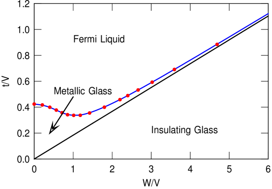
Figure 19: Phase diagram from Typical Medium Theory of Anderson localization tmt, giving $\alpha=1$. The intermediate metallic glass phase shrinks as disorder $W$ grows. Compare this to the Bethe lattice case (Fig. 18), where $\alpha=\infty$.

The intermediate metallic glassy phase still exists, but shrinks as $W\rightarrow\infty$, reflecting the small value of the critical exponent $\alpha=1$, which can be shown analytically within TMT. A more realistic value for this exponent, corresponding to $d=3$, requires more detailed numerical calculations, which remains a challenge for future work.

Low disorder - Mott transition. In the limit of weak disorder $W\ll U,V$, interactions drive the metal-insulator transition. Concentrating on the model at half-filling, the system will undergo a Mott transition mott-book90 as the hopping $t$ is sufficiently reduced. Since for the Mott transition $t_{Mott}(U)\sim U$, near the transition $W\ll t$ and to leading order we can ignore localization effects. In addition, we assume that $V\ll U$ and to leading order the compressibilities have to be calculated with respect to the action $S_{el}$ of a disordered Hubbard model. The simplest formulation that can describe the effects of weak disorder on such a Mott transition is obtained from the dynamical mean-field theory (DMFT) georgesrmp. This formulation, which ignores localization effects, is obtained by rescaling the hopping elements $t\rightarrow t/\sqrt{z}$ and then formally taking the limit of large coordination $z\rightarrow\infty$ (see Section 4). To obtain qualitatively correct analytical results describing the vicinity of the disordered Mott transition at $T=0,$ we have solved the DMFT equations using a 4-boson method mitglass-prl03. At weak disorder, these equations can be easily solved in closed form and we simply report the relevant results. The critical value of hopping for the Mott transition is found to decrease with disorder as

$$t_{c}(W)\approx t_{c}^{o}\,(1-4(W/U)^{2}+\cdots),$$ (108)

where for a simple semi-circular density of states georgesrmp $t_{c}^{o}=3\pi U/64$ (in this model, the bandwidth $B=4t$). Physically, the disorder tends to suppress the Mott insulating state, since it broadens the Hubbard bands and narrows the Mott-Hubbard gap. At sufficiently strong disorder $W\geq U$, the Mott insulator is suppressed even in the atomic limit $t\rightarrow 0$. The behavior of the compressibilities can also be calculated near the Mott transition and to leading order we find

$$\chi^{(2)}=\left[\frac{8}{3\pi t_{c}^{o}}(1-\frac{t_{c}(W)}{t})\right]^{2}(1+28(W/U)^{2}).$$ (109)

Therefore, as with any compressibility, $\chi^{(2)}$ is found to be very small in the vicinity of the Mott transition, even in the presence of finite disorder. As a result, the tendency to glassy ordering is strongly suppressed at weak disorder when one approaches the Mott insulating state.

Finally, having analyzed the limits of weak and strong disorder, we briefly comment on what may be expected in the intermediate region $W\sim U$. The Mott gap cannot exist for $W>U$, so in this region and for sufficiently small $t$ (i. e. kinetic energy), one enters a gapless (compressible) Mott-Anderson insulator. For $W\sim U,$ the computation of $\chi^{(2)}$ requires the full solution of the Mott-Anderson problem. The required calculations can and should be performed using the formulation of motand, but that difficult task is a challenge for the future. However, based on general arguments presented above, we expect $\chi^{(2)}$ to vanish as one approaches the Mott insulator $(W<U)$, but to diverge as one approaches the Mott-Anderson insulator ($W>U).$ Near the tetracritical point, we may expect $\chi^{(2)}\sim\delta W^{-\beta}\delta t^{\alpha},$ where $\delta W=W-W_{Mott}(t)$ is the distance to the Mott transition line, and $\delta t=t-t_{c}(W)$ is the distance to the Mott-Anderson line. Using this Ansatz and Eq. (102), we find the glass transition line to take the form

$$\delta t=t_{G}(W)-t_{c}(W)\sim\delta W^{\beta/\alpha};\;W\sim W_{Mott}.$$ (110)

We thus expect the intermediate metallic glass phase to be suppressed as the disorder is reduced, and one approaches the Mott insulating state. Physically, glassy behavior of electrons corresponds to many low-lying rearrangements of the charge density; such rearrangements are energetically unfavorable close to the (incompressible) Mott insulator, since the on-site repulsion $U$ opposes charge fluctuations. Interestingly, very recent experiments on low density electrons in silicon MOSFETs have revealed the existence of exactly such an intermediate metallic glass phase in low mobility (highly disordered) samples bogdanovich-prl02. In contrast, in high mobility (low disorder) samples JJPRL02, no intermediate metallic glass phase is seen and glassy behavior emerges only as one enters the insulator, consistent with our theory. Similar conclusions have also been reported in studies of highly disordered InO₂ films films22,films23, where the glassy slowing down of the electron dynamics seems to be suppressed as the disorder is reduced and one crosses over from an Anderson-like to a Mott-like insulator. In addition, these experiments bogdanovich-prl02,JJPRL02 provide striking evidence of scale-invariant dynamical correlations inside the glass phase, consistent with the hierarchical picture of glassy dynamics, that generally emerges from mean-field approaches re:Mezard86 such as the one used in this work.

5 Beyond DMFT: loop expansion and diffusion modes

DMFT approaches to correlation and disorder have already provided significant insight in a number of key phenomena and processes around the metal-insulator transition. Most importantly, these methods have made it possible to describe strong correlation effects associated with both “Mottness” and the glassy behavior of electrons. The information provided is, in many ways, rather complementary to the conventional weak-coupling approaches which focused on the effects of long-wavelength diffusion modes within the Fermi liquid picture. Because of their focus on local correlation effects, the DMFT theories are ill-suited to describe those phenomena and regimes where long-range spatial correlations dominate. One of the biggest challenges for future work is to find ways to combine the strength of both approaches and introduce systematic methods to incorporate the non-local spatial correlations ignored by DMFT. While little has been done so far to implement this ambitious program, some approaches have already been outlined that provide guidance on how the problem should be formulated. We conclude our discussion by a brief outline of a promising approach to include both the local correlation processes and the diffusion-mode effects within a single theory.

1 Gauge Invariant Models of Wegner

The task of identifying the leading nonlocal corrections to DMFT can be formulated in a particularly elegant and transparent fashion for certain special models of disorder. Here, the DMFT equations can be obtained dk-prb94 from a functional-integral formulation at the saddle-point level, allowing systematic corrections using a loop expansion. In this class, the inter-site hopping elements are assumed to be random variables of the form

$$t_{ij}=y_{ij}\;g(x_{i},x_{j}),$$ (111)

and in addition, there can be an arbitrary distribution of site energies $\varepsilon_{i}$. Here, $y_{ij}$-s are independent bond variables with a symmetric distribution, i. e. $\overline{y_{ij}^{2n+1}}=0$, and $g(x_{i},x_{j})$ is an arbitrary function of local site variables $x_{i}$.

The special class of models which have a symmetric distribution of hopping elements has a very simple physical interpretation. As first observed by Wegner wegner79,wegner80, in these “gauge invariant” models, the phases of the electrons undergo random shifts at every lattice hop and so the mean free path $\ell$ reduces to one lattice spacing. On general grounds, on length scales longer than $\ell$ the details of the lattice structure are washed out by disorder, so that for gauge invariant models in the large dimensionality limit, the details of the lattice structure become irrelevant. We contrast this with the models with arbitrary disorder discussed previously, which have a well defined pure limit and accordingly can also have an arbitrarily large mean free path. The presence of this intermediate length scale ($\ell$ can be much larger than the lattice spacing $a$, but much smaller than the localization length $\xi$) is often irrelevant to both long-wavelength phenomena such as localization and local phenomena such as the Mott transition. The gauge invariant models avoid these unnecessary complications without disrupting any of the qualitative properties on either very short or very long length scales.

The general properties are the same for all the models in this class, but for the simplicity of our presentation, we will restrict our attention to the separable case shiba71 where $g(x_{i},x_{j})=x_{i}x_{j}$, with an arbitrary distribution $P_{X}(x_{i})$ for the site variables $x_{i}$. For the trivial choice of $P_{X}(x_{i})=\delta(x_{i}-1)$, the models reduce to the gauge invariant models of Wegner wegner79,wegner80. Nontrivial distributions $P_{X}(x_{i})$ which extend to small values of the variable $x_{i}$ are useful for the study of disorder-induced local moment formation milovanovic89. Sites with small $x_{i}$ represent sites with weak hybridization. At intermediate correlations, we expect sites with small $x_{i}$ to behave as local moments and give large contributions to thermodynamic quantities such as the specific heat coefficient $\gamma=C/T$, while other sites remain in the itinerant regime.

Also, we take the $y_{ij}$-s to be Gaussian random variables with zero mean and variance

$$\overline{y_{ij}^{2}}=\frac{1}{z}f_{ij}\;t^{2}.$$ (112)

Here, the (uniform) matrix $f_{ij}$ specifies the lattice structure

$$f_{ij}\;=\;\left\{\begin{array}[]{l}1,\ \mbox{for connected sites,}\\ 0,\ \mbox{for disconnected sites,}\end{array}\right.$$ (113)

and we have scaled the (square of the) hopping elements by the coordination number $z=\sum_{j}f_{ij}$, in order to obtain finite results in the $z\rightarrow\infty$ limit.

2 Functional Integral Formulation

At this point, it is convenient to explicitly perform the averaging over the Gaussian random (bond) variables $y_{ij}$, using the standard replica formulation wegner79,wegner80. The hopping part of the action then assumes the form dk-prb94

$$S_{hop}=\frac{1}{2}t^{2}\;\sum_{ij}\;\frac{1}{z}f_{ij}\;x_{i}^{2}\;x_{j}^{2}\;\left[\sum_{\alpha,s}\int_{o}^{\beta}\,d\tau\,[c^{\dagger\;\alpha}_{s,i}(\tau)c_{s,j}^{\alpha}(\tau)+h.c.]\right]^{2}.$$ (114)

As we can see from this expression, the averaging over disorder has generated a quartic term in the action that is nonlocal in (imaginary) time, spin and replica indices. We are now in a position to introduce collective $Q$-fields wegner79,wegner80,fink-jetp83,fink-jetp84 of the form (in terms of Matsubara frequencies $\omega=2n\pi T$; the indices “n” are omitted for brevity)

$$Q_{\omega_{1}\omega_{2}}^{\alpha_{1}\alpha_{2},s_{1}s_{2}}(i)=\frac{1}{z}\sum_{j}f_{ij}\;x_{j}^{2}\;c^{\dagger\;\alpha_{1}}_{j,s_{1}}(\omega_{1})c^{\alpha_{2}}_{j,s_{2}}(\omega_{2}),$$ (115)

by decoupling the (quartic) hopping term using a Hubbard-Stratonovich transformation. For simplicity, as before, we will ignore the superconducting phases, as well as the fluctuations in the particle-particle (Cooper) channel, so that the $Q$-field does not have anomalous components. The procedure can be straightforwardly generalized to include the omitted terms efetov80.

It is now possible to formally integrate out the electron (Grassmann) fields and the resulting action for the $Q$-fields can be written as

$$S[Q]=S_{hop}[Q]\;+\;S_{loc}[Q].$$ (116)

The nonlocal part of the action $S_{hop}[Q]$ takes a simple quadratic form in terms of the $Q$ fields

$$S_{hop}[Q]=-\frac{1}{2}\;t^{2}\;\sum_{ij}\sum_{\alpha_{1}\alpha_{2}}\sum_{s_{1}s_{2}}\sum_{\omega_{1}\omega_{2}}K_{ij}\;Q_{\omega_{1}\omega_{2}}^{\alpha_{1}\alpha_{2},s_{1}s_{2}}(i)Q_{\omega_{2}\omega_{1}}^{\alpha_{2}\alpha_{1},s_{2}s_{1}}(j),$$ (117)

where, $K_{ij}=\frac{1}{z}f^{-1}_{ij}$ is the inverse lattice matrix, scaled by coordination number $z$. In contrast, all the nonlinearities are contained in the local part of the action

$$S_{loc}[Q]=-\sum_{i}\;\ln\int dx_{i}P_{X}(x_{i})\int d\varepsilon_{i}P_{S}(\varepsilon_{i})\int Dc^{\dagger}_{i}Dc_{i}\exp\left\{-S_{eff}[c^{\dagger}_{i},c_{i},Q_{i},x_{i},\varepsilon_{i}]\right\},$$ (118)

where the local effective action takes the form

$$S_{eff}[c^{\dagger}_{i},c_{i},Q_{i},x_{i},\varepsilon_{i}]=$$

$$-\sum_{\alpha_{1}\alpha_{2}}\sum_{s_{1}s_{2}}\sum_{\omega_{1}\omega_{2}}c^{\dagger\;\alpha_{1}}_{i,s_{1}}(\omega_{1})[\left(i\omega_{1}+\mu-\varepsilon_{i}\right)\delta_{\alpha_{1}\alpha_{2}}\delta_{s_{1}s_{2}}\delta_{\omega_{1}\omega_{2}}-x_{i}^{2}\;t^{2}\,Q_{\omega_{1}\omega_{2}}^{\alpha_{1}\alpha_{2},s_{1}s_{2}}(i)]c^{\alpha_{2}}_{i,s_{2}}(\omega_{2})$$

$$+U\sum_{\alpha}\;\sum_{\omega_{1}+\omega_{3}=\omega_{2}+\omega_{4}}\;c^{\dagger\;\alpha}_{i,\uparrow}(\omega_{1})c^{\alpha}_{i,\uparrow}(\omega_{2})c^{\dagger\;\alpha}_{i,\downarrow}(\omega_{3})c^{\alpha}_{i,\downarrow}(\omega_{4}).$$ (119)

The local effective action $S_{eff}[c^{\dagger}_{i},c_{i},Q_{i},x_{i},\varepsilon_{i}]$ is identical to the action of a (generalized) Anderson impurity model embedded in an electronic bath characterized by a hybridization function $x_{i}^{2}\;t^{2}\,Q_{\omega_{1}\omega_{2}}^{\alpha_{1}\alpha_{2},s_{1}s_{2}}(i)$. We can thus interpret our system as a collection of Anderson impurity models Anderson1961 that are “connected” through the existence of collective $Q$-fields. Here we note that, in contrast to an ordinary Anderson model, the hybridization function is now non-diagonal in frequency, spin and replica indices. Physically, this reflects the fact that in general dimensions a given site can be regarded as an Anderson impurity model in a fluctuating bath which breaks translational invariance in time, space and spin.

3 Saddle-Point Solution

The action has a general form which is very similar to standard lattice models investigated in statistical mechanics goldenfeldbook. As usual, the problem simplifies considerably in the limit of large coordination number, when the spatial fluctuations of the Hubbard-Stratonovich field ($Q$ in our case) are suppressed and the mean-field theory becomes exact. It is worth pointing out that there are two classes of lattices which can have large coordination:

(a) Lattices with short-range bonds but living in a space of large dimensionality. For example, on a hypercubic lattice with nearest neighbor hopping in $d$ dimensions, $z=2d$.

(b) Lattices embedded in a finite dimensional space but having long hopping range. In this case, the lattice matrix $f_{ij}$ takes the form

$$f_{ij}\;=\;\left\{\begin{array}[]{l}1,|i-j|<\,L,\\ 0,\mbox{otherwise,}\end{array}\right.$$ (120)

and the coordination number $z\sim L^{d}$.

In either case, when $z\rightarrow\infty$, the functional integral over $Q$-fields, representing the partition function, can be evaluated (exactly) by a saddle-point method and we obtain a mean-field theory. In order to derive the mean-field equations in our case, we look for extrema of the action $S[Q]$ with respect to variations of the $Q$-fields, i. e.

$$\frac{\delta\,S[Q]}{\delta\,Q_{\omega_{1}\omega_{2}}^{\alpha_{1}\alpha_{2},s_{1}s_{2}}(i)}=0.$$ (121)

Since the saddle-point solution is translationally invariant in time and space and conserves spin, it is diagonal in all indices

$$\left[Q_{\omega_{1}\omega_{2}}^{\alpha_{1}\alpha_{2},s_{1}s_{2}}(i)\right]|_{SP}=\delta_{\alpha_{1}\alpha_{2}}\delta_{s_{1}s_{2}}\delta_{\omega_{1}\omega_{2}}Q^{SP}_{s}(\omega),$$ (122)

and the saddle-point equations assume the form

$$Q_{s}^{SP}(\omega)=\int d\varepsilon_{i}P_{S}(\varepsilon_{i})\int dx_{i}P_{X}(x_{i})\,x_{i}^{2}\;G_{i,s}(\omega),$$ (123)

where

$$G_{i,s}(\omega)=<c^{\dagger}_{s}(\omega)c_{s}(\omega)>_{S_{eff}[c^{\dagger},c,Q^{SP},x_{i},\varepsilon_{i}]}.$$ (124)

If we identify

$$W_{s,i}(\omega)\equiv x_{i}^{2}\,t^{2}Q_{s}^{SP}(\omega),$$ (125)

we see that our saddle-point equations become identical to the standard DMFT ($d\rightarrow\infty$) equations, when applied to the appropriate model of hopping disorder. We emphasize that the present equations are exact at $z\rightarrow\infty$ for an arbitrary lattice, due to the presence of the “gauge invariant” form of the hopping disorder. Since the saddle point equations determine the local effective action, this means that all the local correlation functions will be insensitive to the lattice structure in this mean-field limit. However, other properties such as the tendency to the formation of spin and charge density waves are very sensitive to the details of the lattice structure.

As an example, we can compare the case of simple hopping disorder, $t_{ij}=y_{ij}$, in a bipartite lattice such as the Bethe lattice and the case of a lattice with infinite range hopping (the limit $L\rightarrow\infty$ of the model (b) above). The self-consistency (mean-field) equations are identical in the two cases and in fact reduce to those of a pure Hubbard model on a Bethe lattice with hopping $t$. On the other hand, it is well established re:Rozenberg92 that in the first case the system is unstable towards the formation of an antiferromagnetic ground state, even for arbitrarily small $U/t$, while in the second, the system remains paramagnetic for any $U/t$, due to the large frustration. In many physical systems, such as doped semiconductors paalanen91, disorder introduces large amounts of frustration and magnetic ordering does not occur, even though the system is strongly correlated. In order to study such situations, it is useful to have at hand microscopic models that have a non-magnetic ground state and allow one to study the approach to the metal-insulator transition which occurs at $T=0$.

4 Loop Expansion

The present approach is particularly convenient for the study of the effects of strong correlations on disorder-driven transitions and the interplay of Anderson localization and strong correlations in general. This is especially true since Anderson localization is not present in $d=\infty$ (or infinite range) models and so one has to extend the approach to include spatial fluctuations missing from the mean-field description. In order to systematically study the fluctuation effects, we proceed to carry out an expansion in terms of the deviations of the collective $Q$-fields from their saddle-point value, i. e., in powers of $\delta Q(i)=Q(i)-Q^{SP}$. This procedure, also known as a loop expansion goldenfeldbook has been used in other disordered problems, such as spin-glasses dominicis91, to generate systematic corrections to the mean-field theory. The method is particularly convenient when applied to long-range models dominicis91 (class (b) above), since in that case the loop corrections are ordered by a small parameter $1/z$. The loop expansion can be applied also to large dimensionality models, but in that case a given order in a loop expansion can be considered to be an infinite resummation of the simple $1/d$ expansion Georges90, since each term contains all powers of $1/d$.

When the expansion of the effective action in terms of $\delta Q$-s is carried to lowest, quadratic order, we obtain a theory describing gaussian fluctuations around the saddle point, which represent weakly interacting collective modes wegner79,wegner80,fink-jetp83,fink-jetp84. Higher order terms in the expansion then generate effective interactions of these modes, which under appropriate conditions can lead to fluctuation-driven phase transitions. In practice, if all the components of the collective $Q$-fields are retained in this analysis, the theory becomes prohibitively complicated and cumbersome. However, in order to analyze the critical behavior, it is not necessary to keep track of all the degrees of freedom, but it suffices to limit the analysis to soft modes, i. e., those that represent low energy excitations. In disordered metallic phases, charge and spin conservation laws lead to the existence of diffusion modes, which are the hydrodynamic modes describing charge- and spin-density relaxation. In the Fermi liquid regime ckl, all the other collective excitations require higher energy and can be neglected in a hydrodynamic description of the system. One is then led to construct a theory of interacting diffusion modes, as a theory of critical phenomena for disordered interacting systems.

This line of reasoning was used in field-theoretical approaches to the localization problem of noninteracting electrons, as first developed by Wegner wegner79,wegner80. In this theory, collective $Q$-fields, similar to the ones presented in this paper, are introduced. At the saddle-point level, no phase transition occurs and all the states are extended. An analysis of the fluctuations of the $Q$-fields is then performed and a subset of those fluctuations identified, which represent the hydrodynamic (diffusion) modes. Only the fluctuations of these modes are retained and an effective hydrodynamic theory is constructed - the non-linear sigma model wegner79,wegner80 . The interactions of these modes lead to the metal-insulator (localization) transition, which was analyzed using renormalization-group techniques and $2+\varepsilon$ expansions. In subsequent work, Finkelshtein fink-jetp83,fink-jetp84 was able to apply a similar procedure to interacting disordered electrons. However, this theory is based on a number of implicit assumptions that restrict its validity to Fermi-liquid regimes. In the language of $Q$-fields, this theory again expands around a noninteracting saddle-point and the interaction effects appear only at the level of the fluctuation corrections.

When strongly correlated electronic systems are considered, much of the physics relates precisely to the destruction of coherent quasiparticles by inelastic processes, so that one needs a description that is not limited to Fermi-liquid regimes. In the language of hydrodynamics, new soft modes appear, which indicate the tendency towards interaction-driven instabilities. In particular, strong correlations can lead to local moment formation and the Mott transition. In both cases, charge fluctuations are suppressed and low-energy spin fluctuations dominate the physics.

In the present approach, in contrast to the work of Wegner and Finkelshtein, the strong correlations are treated in a non-perturbative fashion already at the saddle-point (mean-field) level, so that all the soft modes can be systematically included. In particular, even at the one-loop level, we can address the question of how the disorder-induced local moment formation and the approach to the Mott transition affect the weak localization (diffusion) corrections. Ultimately, our approach indicates how a more general low energy theory can be constructed that extends the $\sigma$-model description so as to include strong correlation effects.

In the present discussion, we will limit our attention to the form of the Gaussian fluctuations of the $Q$-fields, which allow one in principle to compute the leading corrections to mean-field theory. The Gaussian part of the action takes the form

$$S^{(2)}[Q] = -\frac{1}{2}\,t^{2}\,\sum_{l_{1}\cdots l_{4}}\int\frac{dk}{(2\pi)^{d}}\,\delta Q_{l_{1}l_{2}}(k)\left[\left(L^{2}k^{2}+1\right)\delta_{l_{1}l_{4}}\delta_{l_{2}l_{3}}\right.$$ (126)

$$\left.-t^{2}W(l_{1})W(l_{3})\delta_{l_{1}l_{2}}\delta_{l_{3}l_{4}}+t^{2}\Gamma(l_{1}\cdots l_{4})\right]\,\delta Q_{l_{3}l_{4}}(-k).$$

This expression is appropriate for the long-ranged model (b) above, in which case the inverse lattice matrix in momentum space takes the form $K(k)\approx 1+L^{2}k^{2}$ and we cut off the momentum integrals at $\Lambda=2\pi/L$. Note that the coefficient of $k^{2}$, which can be interpreted as the stiffness of the $\delta Q$ modes, is $\sim L^{2}$, so we see that indeed the fluctuations are suppressed at $L\rightarrow\infty$. In the above formula, the index $l_{m}$ is used to represent the frequency, spin and replica indices. The local vertex function $\Gamma(l_{1}\cdots l_{4})$ is given by

$$\Gamma(l_{1}\cdots l_{4})=\int d\varepsilon_{i}P_{S}(\varepsilon_{i})\int dx_{i}P_{X}(x_{i})\,x_{i}^{4}<c^{\dagger}_{i}(l_{1})c_{i}(l_{2})c^{\dagger}_{i}(l_{3})c_{i}(l_{4})>_{S_{eff}[Q^{SP}]}.$$ (127)

At this level, the dynamics of the collective fluctuations $\delta Q$ is governed by the form of $S^{(2)}[\delta Q]$, which is expressed in terms of the local correlation functions of the saddle-point theory, i. e., of the $d=\infty$ disordered Hubbard model. Accordingly, a detailed study of the $d=\infty$ limit does not provide only a mean-field description of the problem, but also determines the form of the leading corrections resulting from fluctuations. Extensions of the theory to include the effects of these fluctuation corrections remain to be addressed in more detail in future work.

6 Acknowledgments

This work was supported by FAPESP through grant 07/57630-5 (EM), CNPq through grant 304311/2010-3 (EM), and by NSF through grants DMR-0542026 and DMR-1005751. (VD).

References

- Abou-Chacra et al. (1973) Abou-Chacra, R., Anderson, P. W., and Thouless, D. J. (1973). J. Phys. C, 6, 1734.
- Abrahams et al. (2001) Abrahams, E., Kravchenko, S. V., and Sarachik, M. P. (2001). Rev. Mod. Phys., 73, 251–266.
- Aguiar et al. (2005) Aguiar, M. C. O., Dobrosavljević, V., Abrahams, E., and Kotliar, G. (2005). Phys. Rev. B, 71, 205115.
- Aguiar et al. (2006) Aguiar, M. C. O., Dobrosavljević, V., Abrahams, E., and Kotliar, G. (2006). Phys. Rev. B, 73, 115117.
- Aguiar et al. (2009) Aguiar, M. C. O., Dobrosavljević, V., Abrahams, E., and Kotliar, G. (2009). Phys. Rev. Lett., 102, 156402.
- Aguiar et al. (2003) Aguiar, M. C. O., Miranda, E., and Dobrosavljević, V. (2003). Phys. Rev. B, 68, 125104.
- Aguiar et al. (2004) Aguiar, M. C. O., Miranda, E., Dobrosavljević, V., Abrahams, E., and Kotliar, G. (2004). Europhys. Lett., 67, 226.
- Alloul et al. (2009) Alloul, H., Bobroff, J., Gabay, M., and Hirschfeld, P. J. (2009). Rev. Mod. Phys., 81, 45.
- Altshuler and Aronov (1979) Altshuler, B. L. and Aronov, A. G. (1979). Solid State Commun., 30, 115.
- Anderson (1958) Anderson, P. W. (1958). Phys. Rev., 109, 1492.
- Anderson (1961) Anderson, P. W. (1961). Phys. Rev., 124, 41.
- Anderson (1978) Anderson, P. W. (1978). Rev. Mod. Phys., 50, 191.
- Anderson and Yuval (1969) Anderson, P. W. and Yuval, G. (1969). Phys. Rev. Lett., 23, 89.
- Anderson et al. (1970) Anderson, P. W., Yuval, G., and Hamman, D. R. (1970). Phys. Rev. B, 1, 4464.
- Andrade et al. (2009a) Andrade, E. C., Miranda, E., and Dobrosavljević, V. (2009a). Phys. Rev. Lett., 102, 206403.
- Andrade et al. (2009b) Andrade, E. C., Miranda, E., and Dobrosavljevic, V. (2009b). Physica B: Condensed Matter, 404, 3167.
- Andrade et al. (2010) Andrade, E. C., Miranda, E., and Dobrosavljević, V. (2010). Phys. Rev. Lett., 104, 236401.
- Aronson et al. (1995) Aronson, M. C., Obsorn, R., Robinson, R. A., Lynn, J. W., Chau, R., Seaman, C. L., and Maple, M. B. (1995). Phys. Rev. Lett., 75, 725.
- Arrachea et al. (2004) Arrachea, L., Dalidovich, D., Dobrosavljević, V., and Rozenberg, M. J. (2004). Phys. Rev. B, 69, 064419.
- Balatsky et al. (2006) Balatsky, A. V., Vekhter, I., and Zhu, Jian-Xin (2006). Rev. Mod. Phys., 78, 373.
- Belitz and Kirkpatrick (1995) Belitz, D. and Kirkpatrick, T. R. (1995). Phys. Rev. B, 52, 13922.
- Ben-Chorin et al. (1993) Ben-Chorin, M., Ovadyahu, Z., and Pollak, M. (1993). Phys. Rev. B, 48, 15025.
- Bernal et al. (1995) Bernal, O. O., MacLaughlin, D. E., Lukefahr, H. G., and Andraka, B. (1995). Phys. Rev. Lett., 75, 2023.
- Bogdanovich and Popović (2002) Bogdanovich, S. and Popović, D. (2002). Phys. Rev. Lett., 88, 236401.
- Borghi et al. (2009) Borghi, G., Fabrizio, M., and Tosatti, E. (2009). Phys. Rev. Lett., 102, 066806.
- Borghi et al. (2010) Borghi, G., Fabrizio, M., and Tosatti, E. (2010). Phys. Rev. B, 81, 115134.
- Bray and Moore (1980) Bray, A. J. and Moore, M. A. (1980). J. Phys. C, 13, L655.
- Brinkman and Rice (1970) Brinkman, W. F. and Rice, T. M. (1970). Phys. Rev. B, 2, 4302.
- Burdin et al. (2002) Burdin, S., Grempel, D. R., and Georges, A. (2002). Phys. Rev. B, 66, 045111.
- Byczuk (2005) Byczuk, K. (2005). Phys. Rev. B, 71, 205105.
- Byczuk et al. (2005) Byczuk, K., Hofstetter, W., and Vollhardt, D. (2005). Phys. Rev. Lett., 94, 056404.
- Byczuk et al. (2009a) Byczuk, K., Hofstetter, W., and Vollhardt, D. (2009a). Phys. Rev. Lett., 102, 146403.
- Byczuk et al. (2009b) Byczuk, K., Hofstetter, W., Yu, U., and Vollhardt, D. (2009b). The European Physical Journal - Special Topics, 180, 135.
- Camjayi and Rozenberg (2003) Camjayi, A. and Rozenberg, M. J. (2003). Phys. Rev. Lett., 90, 217202.
- Castellani et al. (1987) Castellani, C., Kotliar, B. G., and Lee, P. A. (1987). Phys. Rev. Lett., 56, 1179.
- Castro Neto et al. (1998) Castro Neto, A. H., Castilla, G., and Jones, B. A. (1998). Phys. Rev. Lett., 81, 3531.
- Castro Neto and Jones (2000) Castro Neto, A. H. and Jones, B. A. (2000). Phys. Rev. B, 62, 14975.
- Chakravarty et al. (1999) Chakravarty, S., Kivelson, S., Nayak, C., and Voelker, K. (1999). Phil. Mag. B, 79, 859.
- Chen and Freericks (2007) Chen, L. and Freericks, J. K. (2007). Phys. Rev. B, 75, 125114.
- Chitra and Kotliar (2000) Chitra, R. and Kotliar, G. (2000). Phys. Rev. Lett., 84, 3678.
- Coleman (1987) Coleman, P. (1987). Phys. Rev. B, 35, 5072.
- Coleman and Andrei (1987) Coleman, P. and Andrei, N. (1987). J. Phys.: Condens. Matter, 1, 4057.
- Cummins et al. (1994) Cummins, H. Z., Li, G., Du, W. M., and Hernandez, J. (1994). Physica A, 204, 169.
- Dalidovich and Dobrosavljević (2002) Dalidovich, D. and Dobrosavljević, V. (2002). Phys. Rev. B, 66, 081107.
- Davies et al. (1982) Davies, J. H., Lee, P. A., and Rice, T. M. (1982). Phys. Rev. Lett., 49, 758.
- de Almeida and Thouless (1978) de Almeida, J. R. L. and Thouless, D. J. (1978). J. Phys. A, 11, 983.
- de Andrade et al. (1998) de Andrade, M. C., Chau, R., Dickey, R. P., Dilley, N. R., Freeman, E. J., Gajewski, D. A., Maple, M. B., Movshovich, R., Neto, A. H. Castro, Castilla, G., and Jones, B. A. (1998). Phys. Rev. Lett., 81, 5620.
- de Dominicis, C. et al. (1991) de Dominicis, C., Kondor, C. I., and Temisvari, T. (1991). J. de Physique I, A24, L301.
- Demler et al. (2002) Demler, E., Nayak, C., Kee, H.-Y., Kim, Y.-B., and Senthil, T. (2002). Phys. Rev. B, 65, 155103.
- Dobrosavljević (2010) Dobrosavljević, V. (2010). Int. Jour. Mod. Phys. B, 24, 1680.
- Dobrosavljević et al. (1997) Dobrosavljević, V., Abrahams, E., Miranda, E., and Chakravarty, S. (1997). Phys. Rev. Lett., 79, 455.
- Dobrosavljević et al. (1992) Dobrosavljević, V., Kirkpatrick, T. R., and Kotliar, B. G. (1992). Phys. Rev. Lett., 69, 1113.
- Dobrosavljević and Kotliar (1993) Dobrosavljević, V. and Kotliar, G. (1993). Phys. Rev. Lett., 71, 3218.
- Dobrosavljević and Kotliar (1994) Dobrosavljević, V. and Kotliar, G. (1994). Phys. Rev. B, 50, 1430.
- Dobrosavljević and Kotliar (1997) Dobrosavljević, V. and Kotliar, G. (1997). Phys. Rev. Lett., 78, 3943.
- Dobrosavljević and Kotliar (1998) Dobrosavljević, V. and Kotliar, G. (1998). Phil. Trans. R. Soc. Lond. A, 356, 1.
- Dobrosavljević et al. (2003a) Dobrosavljević, V., Pastor, A. A., and Nikolić, B. K. (2003a). Europhys. Lett., 62, 76.
- Dobrosavljević and Stratt (1987) Dobrosavljević, V. and Stratt, R. M. (1987). Phys. Rev. B, 36, 8484.
- Dobrosavljević et al. (2003b) Dobrosavljević, V., Tanasković, D., and Pastor, A. A. (2003b). Phys. Rev. Lett., 90, 016402.
- Doniach (1977) Doniach, S. (1977). Physica B, 91, 231.
- Economou (2006) Economou, E. N. (2006). Green’s Functions in Quantum Physics. Springer, Berlin.
- Efetov et al. (1980) Efetov, K. B., Larkin, A. I., and Khmel’nitskii, D. E. (1980). Zh. Eksp. Teor. Fiz., 79, 1120.
- Efros (1992) Efros, A. L. (1992). Phys. Rev. Lett., 68, 2208.
- Efros and Shklovskii (1975) Efros, A. L. and Shklovskii, B. I. (1975). J. Phys. C, 8, L49.
- Elliott et al. (1974) Elliott, R. J., Krumhansl, J. A., and Leath, P. L. (1974). Rev. Mod. Phys., 46, 465.
- Finkel’stein (1983) Finkel’stein, A. M. (1983). Zh. Eksp. Teor. Fiz., 84, 168. [Sov. Phys. JETP 57, 97 (1983)].
- Finkel’stein (1984) Finkel’stein, A. M. (1984). Zh. Eksp. Teor. Fiz., 86, 367. [Sov. Phys. JETP 59, 212 (1983)].
- Fisher (1992) Fisher, D. S. (1992). Phys. Rev. Lett., 69, 534.
- Fisher (1994) Fisher, D. S. (1994). Phys. Rev. B, 50, 3799.
- Fisher (1995) Fisher, D. S. (1995). Phys. Rev. B, 51, 6411.
- Fisher and Huse (1986) Fisher, D. S. and Huse, D.A. (1986). Phys. Rev. Lett., 56, 1601.
- Fisher and Young (1998) Fisher, D. S. and Young, A. P. (1998). Phys. Rev. B, 58, 9131.
- Fradkin (1991) Fradkin, E. (1991). Field Theories of Condensed Matter Systems. Adisson-Wesley, Redwood City, California.
- Freericks (2004) Freericks, J. K. (2004). Phys. Rev. B, 70, 195342.
- Georges and Kotliar (1992) Georges, A. and Kotliar, G. (1992). Phys. Rev. B, 45, 6479.
- Georges et al. (1996) Georges, A., Kotliar, G., Krauth, W., and Rozenberg, M. J. (1996). Rev. Mod. Phys., 68, 13.
- Georges et al. (1990) Georges, A., Mezard, M., and Yedida, J. S. (1990). Phys. Rev. Lett., 64, 2937.
- Georges et al. (2001) Georges, A., Parcollet, O., and Sachdev, S. (2001). Phys. Rev. B, 63, 134406.
- Goldenfeld (1992) Goldenfeld, N. (1992). Lectures on phase transitions and the renormalization group. Addison-Wesley, Reading.
- Grannan and Yu (1993) Grannan, E. R. and Yu, C. C. (1993). Phys. Rev. Lett., 71, 3335.
- Grewe and Steglich (1991) Grewe, N. and Steglich, F. (1991). In Handbook on the Physics and Chemistry of Rare Earths (ed. K. A. Geschneider Jr. and L. Eyring), Volume 14, p. 343. Elsevier, Amsterdam.
- Griffiths (1969) Griffiths, R. B. (1969). Phys. Rev. Lett., 23, 17.
- Guo et al. (1996) Guo, M., Bhatt, R. N., and Huse, D. A. (1996). Phys. Rev. B, 54, 3336.
- Gutzwiller (1963) Gutzwiller, M. C. (1963). Phys. Rev. Lett., 10, 159.
- Gutzwiller (1964) Gutzwiller, M. C. (1964). Phys. Rev., 134, A923.
- Gutzwiller (1965) Gutzwiller, M. C. (1965). Phys. Rev., 137, A1726.
- Helmes et al. (2008) Helmes, R. W., Costi, T. A., and Rosch, A. (2008). Phys. Rev. Lett., 101, 066802.
- Herbut (2001) Herbut, I. F. (2001). Phys. Rev. B, 63, 113102.
- Hertz (1976) Hertz, J. A. (1976). Phys. Rev. B, 14, 1165.
- Hewson (1993) Hewson, A. C. (1993). The Kondo Problem to Heavy Fermions. Cambrige University Press, Cambridge.
- Hoyos et al. (2007) Hoyos, J. A., Kotabage, C., and Vojta, T. (2007). Phys. Rev. Lett., 99, 230601.
- Hoyos and Vojta (2006) Hoyos, J. A. and Vojta, T. (2006). Phys. Rev. B, 74, 140401(R).
- Hoyos and Vojta (2008) Hoyos, J. A. and Vojta, T. (2008). Phys. Rev. Lett., 100, 240601.
- Hubbard (1963) Hubbard, J. (1963). Proc. R. Soc. (London) A, 276, 238.
- Hyman and Yang (1997) Hyman, R. A. and Yang, K. (1997). Phys. Rev. Lett., 78, 1783.
- Hyman et al. (1996) Hyman, R. A., Yang, K., Bhatt, R. N., and Girvin, S. M. (1996). Phys. Rev. Lett., 76, 839.
- Jacko et al. (2009) Jacko, A. C., FjÊrestad, J. O., and Powell, B. J. (2009). Nature Physics, 5, 422.
- Jagannathan et al. (1988) Jagannathan, A., Abrahams, E., and Stephen, M. J. (1988). Phys. Rev. B, 37, 436.
- Janis et al. (1993) Janis, V., Ulmke, M., and Vollhardt, D. (1993). EPL (Europhysics Letters), 24, 287.
- Janis and Vollhardt (1992) Janis, V. and Vollhardt, D. (1992). Phys. Rev. B, 46, 15712.
- Janssen (1998) Janssen, M. (1998). Phys. Rep., 295, 1.
- Jaroszyński et al. (2002) Jaroszyński, J., Popović, D., and Klapwijk, T. M. (2002). Phys. Rev. Lett., 89, 276401.
- Kadowaki and Woods (1986) Kadowaki, K. and Woods, S. B. (1986). Solid State Commun., 58, 507.
- Kagan et al. (1992) Kagan, Yu., Kikoin, K. A., and Prokof’ev, N. V. (1992). Physica B, 182, 201.
- Kagawa et al. (2005) Kagawa, F., Miyagawa, K., and Kanoda, K. (2005). Nature, 436, 534.
- Kajueter and Kotliar (1996) Kajueter, H. and Kotliar, G. (1996). Phys. Rev. Lett., 77, 131.
- Kasuya (1956) Kasuya, T. (1956). Progr. Theoret. Phys., 16, 45.
- Kondo (1964) Kondo, J. (1964). Prog. Theor. Phys., 32, 37.
- Kosterlitz (1976) Kosterlitz, J. M. (1976). Phys. Rev. Lett., 37, 1577.
- Kotliar et al. (2000) Kotliar, G., Lange, E., and Rozenberg, M. J. (2000). Phys. Rev. Lett., 84, 5180.
- Kotliar et al. (2002) Kotliar, G., Murthy, S., and Rozenberg, M. J. (2002). Phys. Rev. Lett., 89, 046401.
- Kotliar and Ruckenstein (1986) Kotliar, G. and Ruckenstein, A. E. (1986). Phys. Rev. Lett., 57, 1362.
- Landau (1957a) Landau, L. D. (1957a). Sov. Phys. JETP, 5, 101.
- Landau (1957b) Landau, L. D. (1957b). Sov. Phys. JETP, 3, 920.
- Landau (1959) Landau, L. D. (1959). Sov. Phys. JETP, 8, 70.
- Leggett et al. (1987) Leggett, A. J., Chakravarty, S., Dorsey, A. T., Fisher, M. P. A., Garg, A., and Zwerger, W. (1987). Rev. Mod. Phys., 59, 1.
- Liebsch (2003) Liebsch, A. (2003). Phys. Rev. Lett., 90, 096401.
- Lifshits et al. (1988) Lifshits, I. M., Gredeskul, S. A., and Pastur, L. A. (1988). Introduction to the theory of disordered systems. Wiley, New York.
- Limelette et al. (2003a) Limelette, P., Georges, A., Jerome, D., Wzietek, P., Metcalf, P., and Honig, J. M. (2003a). Science, 302, 89.
- Limelette et al. (2003b) Limelette, P., Wzietek, P., Florens, S., Georges, A., Costi, T. A., Pasquier, C., Jerome, D., Meziere, C., and Batail, P. (2003b). Phys. Rev. Lett., 91, 016401.
- MacLaughlin et al. (2001) MacLaughlin, D. E., Bernal, O. O., Heffner, R. H., Nieuwenhuys, G. J., Rose, M. S., Sonier, J. E., Andraka, B., Chau, R., and Maple, M. B. (2001). Phys. Rev. Lett., 87, 066402.
- Massey and Lee (1996) Massey, J. G. and Lee, M. (1996). Phys. Rev. Lett., 77, 3399.
- McElroy et al. (2005) McElroy, K., Lee, Jinho, Slezak, J. A., Lee, D.-H., Eisaki, H., Uchida, S., and Davis, J. C. (2005). Science, 309, 1048.
- Metzner and Vollhardt (1989) Metzner, W. and Vollhardt, D. (1989). Phys. Rev. Lett., 62, 324.
- Mézard et al. (1986) Mézard, M., Parisi, G., and Virasoro, M. A. (1986). Spin Glass theory and beyond. World Scientific, Singapore.
- Mézard and Young (1992) Mézard, M. and Young, A. P. (1992). Europhys. Lett., 18, 653.
- Miller and Huse (1993) Miller, J. and Huse, D. A. (1993). Phys. Rev. Lett., 70, 3147.
- Millis (1993) Millis, A. J. (1993). Phys. Rev. B, 48, 7183.
- Millis and Lee (1987) Millis, A. J. and Lee, P. A. (1987). Phys. Rev. B, 35, 3394.
- Millis et al. (2002) Millis, A. J., Morr, D. K., and Schmalian, J. (2002). Phys. Rev. B, 66, 174433.
- Milovanović et al. (1989) Milovanović, M., Sachdev, S., and Bhatt, R. N. (1989). Phys. Rev. Lett., 63, 82.
- Miranda and Dobrosavljević (1999) Miranda, E. and Dobrosavljević, V. (1999). Physica B, 259-261, 359.
- Miranda and Dobrosavljević (2001) Miranda, E. and Dobrosavljević, V. (2001). Phys. Rev. Lett., 86, 264.
- Miranda and Dobrosavljević (2005) Miranda, E. and Dobrosavljević, V. (2005). Rep. Prog. Phys., 68, 2337.
- Miranda et al. (1996) Miranda, E., Dobrosavljević, V., and Kotliar, G. (1996). J. Phys.: Condens. Matter, 8, 9871.
- Miranda et al. (1997a) Miranda, E., Dobrosavljević, V., and Kotliar, G. (1997a). Phys. Rev. Lett., 78, 290.
- Miranda et al. (1997b) Miranda, E., Dobrosavljević, V., and Kotliar, G. (1997b). Physica B, 230, 569.
- Mirlin (2000) Mirlin, A. D. (2000). Phys. Rep., 326, 259.
- Mirlin and Fyodorov (1991) Mirlin, A. D. and Fyodorov, Y. V. (1991). Nucl. Phys. B, 366, 507.
- Miyake et al. (1989) Miyake, K., Matsuura, T., and Varma, C.M. (1989). Solid State Commun., 71, 1149.
- Mo et al. (2003) Mo, S.-K., Denlinger, J. D., Kim, H.-D., Park, J.-H., Allen, J. W., Sekiyama, A., Yamasaki, A., Kadono, K., Suga, S., Saitoh, Y., Muro, T., Metcalf, P., Keller, G., Held, K., Eyert, V., Anisimov, V. I., and Vollhardt, D. (2003). Phys. Rev. Lett., 90, 186403.
- Mooij (1973) Mooij, J. H. (1973). Phys. Status Solidi A, 17, 521.
- Motrunich et al. (2001) Motrunich, O., Mau, S.-C., Huse, D. A., and Fisher, D. S. (2001). Phys. Rev. B, 61, 1160.
- Mott (1949) Mott, N. F. (1949). Proc. Roy. Soc. (London), A197, 269.
- Mott (1990) Mott, N. F. (1990). Metal-Insulator Transition. Taylor & Francis, London.
- Müller and Ioffe (2004) Müller, M. and Ioffe, L. B. (2004). Phys. Rev. Lett., 93, 256403.
- Müller and Pankov (2007) Müller, M. and Pankov, S. (2007). Phys. Rev. B, 75, 144201.
- Narayanan et al. (1999a) Narayanan, R., Vojta, T., Belitz, D., and Kirkpatrick, T. R. (1999a). Phys. Rev. B, 60, 10150.
- Narayanan et al. (1999b) Narayanan, R., Vojta, T., Belitz, D., and Kirkpatrick, T. R. (1999b). Phys. Rev. Lett., 82, 5132.
- Narozhny et al. (2001) Narozhny, B. N., Aleiner, I. L., and Larkin, A. I. (2001). Phys. Rev. B, 62, 14898.
- Nattermann (1997) Nattermann, T. (1997). cond-mat/9705295.
- Nozières (1974) Nozières, P. (1974). J. Low Temp. Phys., 17, 31.
- Ohtomo et al. (2002) Ohtomo, A., Muller, D. A., Grazul, J. L., and Hwang, H. Y. (2002). Nature, 419, 378.
- Okamoto and Millis (2004a) Okamoto, S. and Millis, A. J. (2004a). Nature, 428, 630.
- Okamoto and Millis (2004b) Okamoto, S. and Millis, A. J. (2004b). Phys. Rev. B, 70, 241104.
- Ovadyahu and Pollak (1997) Ovadyahu, Z. and Pollak, M. (1997). Phys. Rev. Lett., 79, 459.
- Paalanen and Bhatt (1991) Paalanen, M. A. and Bhatt, R. N. (1991). Physica B, 169, 231.
- Palmer and Pond (1979) Palmer, R. G. and Pond, C. M. (1979). J. Phys. F, 9, 1451.
- Panagopoulos and Dobrosavljević (2005) Panagopoulos, C. and Dobrosavljević, V. (2005). Phys. Rev. B, 72, 014536.
- Pankov (2006) Pankov, S. (2006). Phys. Rev. Lett., 96, 197204.
- Pankov and Dobrosavljević (2005) Pankov, S. and Dobrosavljević, V. (2005). Phys. Rev. Lett., 94, 046402.
- Parcollet and Georges (1999) Parcollet, O. and Georges, A. (1999). Phys. Rev. B, 59, 5341.
- Pastor and Dobrosavljević (1999) Pastor, A. A. and Dobrosavljević, V. (1999). Phys. Rev. Lett., 83, 4642.
- Pastor et al. (2002) Pastor, A. A., Dobrosavreljević, V., and Horbach, M. L. (2002). Phys. Rev. B, 66, 014413.
- Pazmandi et al. (1999) Pazmandi, F., Zarand, G., and Zimanyi, G. T. (1999). Phys. Rev. Lett., 83, 1034.
- Pezzoli and Becca (2010) Pezzoli, M. E. and Becca, F. (2010). Phys. Rev. B, 81, 075106.
- Pezzoli et al. (2009) Pezzoli, M. E., Becca, F., Fabrizio, M., and Santoro, G. (2009). Phys. Rev. B, 79, 033111.
- Pich et al. (1998) Pich, C., Young, A. P., Rieger, H., and Kawashima, N. (1998). Phys. Rev. Lett., 81, 5916.
- Plefka (1982) Plefka, T. (1982). J. Phys. A, 15, 1971.
- Pollak and Hunt (1991) Pollak, M. and Hunt, A. (1991). In Hopping Transport in Solids (ed. M. Pollak and B. I. Shklovskii), pp. 175–206. Elsevier, Amsterdam.
- Potthoff and Nolting (1999) Potthoff, M. and Nolting, W. (1999). Phys. Rev. B, 60, 7834.
- Pruschke et al. (1995) Pruschke, T., Jarrell, M., and Freericks, J. K. (1995). Adv. Phys., 44, 187.
- Read and Newns (1983) Read, N. and Newns, D. M. (1983). J. Phys. C, 16, L1055.
- Read et al. (1995) Read, N., Sachdev, S., and Ye, J. (1995). Phys. Rev. B, 52, 384.
- Refael et al. (2002) Refael, G., Kehrein, S., and Fisher, D. S. (2002). Phys. Rev. B, 66, 060402(R).
- Rodolakis et al. (2009) Rodolakis, F., Mansart, B., Papalazarou, E., Gorovikov, S., Vilmercati, P., Petaccia, L., Goldoni, A., Rueff, J. P., Lupi, S., Metcalf, P., and Marsi, M. (2009). Phys. Rev. Lett., 102, 066805.
- Rozenberg et al. (1999) Rozenberg, M. J., Chitra, R., and Kotliar, G. (1999). Phys. Rev. Lett., 83, 3498.
- Rozenberg and Grempel (1998) Rozenberg, M. J. and Grempel, D. (1998). Phys. Rev. Lett., 81, 2550.
- Rozenberg and Grempel (1999) Rozenberg, M. J. and Grempel, D. (1999). Phys. Rev. B, 60, 4702.
- Rozenberg et al. (1996) Rozenberg, M. J., Kotliar, G., and Kajueter, H. (1996). Phys. Rev. B, 54, 8542.
- Rozenberg et al. (1992) Rozenberg, M. J., Zhang, X. Y., and Kotliar, G. (1992). Phys. Rev. Lett., 69, 1236.
- Ruderman and Kittel (1954) Ruderman, M. A. and Kittel, C. (1954). Phys. Rev., 96, 99.
- Sachdev et al. (1995) Sachdev, S., Read, N., and Oppermann, R. (1995). Phys. Rev. B, 52, 10286.
- Sachdev and Ye (1993) Sachdev, S. and Ye, J. (1993). Phys. Rev. Lett., 70, 3339.
- Sarvestani et al. (1995) Sarvestani, M., Schreiber, M., and Vojta, T. (1995). Phys. Rev. B, 52, R3820.
- Schaffer and Wegner (1980) Schaffer, L. and Wegner, F. (1980). Phys. Rev. B, 38, 113.
- Schrieffer and Wolff (1966) Schrieffer, J. R. and Wolff, P. A. (1966). Phys. Rev., 149, 491.
- Schubert et al. (2010) Schubert, G, Schleede, J., Byczuk, K., Fehske, H., and Vollhardt, D. (2010). Phys. Rev. B, 81, 155106.
- Schwieger et al. (2003) Schwieger, S., Potthoff, M., and Nolting, W. (2003). Phys. Rev. B, 67, 165408.
- Sekiyama et al. (2000) Sekiyama, A., Iwasaki, T., Matsuda, K., Saitoh, Y., ‘nuki, Y, and Suga, S. (2000). Nature, 403, 396.
- Semmler et al. (2010a) Semmler, D., Byczuk, K., and Hofstetter, W. (2010a). Phys. Rev. B, 81, 115111.
- Semmler et al. (2010b) Semmler, D., Wernsdorfer, J., Bissbort, U., Byczuk, K., and Hofstetter, W. (2010b). Phys. Rev. B, 82, 235115.
- Sengupta (2000) Sengupta, A. M. (2000). Phys. Rev. B, 61, 4041.
- Sengupta and Georges (1995) Sengupta, A. M. and Georges, A. (1995). Phys. Rev. B, 52, 10295.
- Senthil et al. (2003) Senthil, T., Sachdev, S., and Vojta, M. (2003). Phys. Rev. Lett., 90, 216403.
- Senthil et al. (2004) Senthil, T., Vojta, M., and Sachdev, S. (2004). Phys. Rev. B, 69, 035111.
- Shiba (1971) Shiba, H. (1971). Prog. Teor. Phys., 46, 77.
- Si et al. (2001) Si, Q., Rabello, S., Ingersent, K., and Smith, J. L. (2001). Nature, 413, 804.
- Si and Smith (1996) Si, Q. and Smith, J. L. (1996). Phys. Rev. Lett., 77, 3391.
- Singh et al. (1998) Singh, A., Ulmke, M., and Vollhardt, D. (1998). Phys. Rev. B, 58, 8683.
- Slater (1951) Slater, J. C. (1951). Phys. Rev., 82, 538.
- Slevin and Ohtsuki (1999) Slevin, K. and Ohtsuki, T. (1999). Phys. Rev. Lett., 82, 382.
- Smith and Si (2000) Smith, J. L. and Si, Q. (2000). Phys. Rev. B, 61, 5184.
- Snoek et al. (2008) Snoek, M., Titvinidze, I., Toke, C., Byczuk, K., and Hofstetter, W. (2008). New Journal of Physics, 10, 093008.
- Song et al. (2008) Song, Y., Wortis, R., and Atkinson, W. A. (2008). Phys. Rev. B, 77, 054202.
- Stewart (1984) Stewart, G. R. (1984). Rev. Mod. Phys., 56, 755.
- Stewart (2001) Stewart, G. R. (2001). Rev. Mod. Phys., 73, 797.
- Stewart (2006) Stewart, G. R. (2006). Rev. Mod. Phys., 78, 743.
- Tanasković et al. (2003) Tanasković, D., Dobrosavljević, V., Abrahams, E., and Kotliar, G. (2003). Phys. Rev. Lett., 91, 066603.
- Tanasković et al. (2005) Tanasković, D., Dobrosavljević, V., and Miranda, E. (2005). Phys. Rev. Lett., 95, 167204.
- Tanasković et al. (2004) Tanasković, D., Miranda, E., and Dobrosavljević, V. (2004). Phys. Rev. B, 70, 205108.
- Terletska et al. (2011) Terletska, H., Vučičević, J., Tanasković, D., and Dobrosavljević, V. (2011). Phys. Rev. Lett., 107, 026401.
- Ting et al. (1975) Ting, C. S., Lee, T. K., and Quinn, J. J. (1975). Phys. Rev. Lett., 34, 870.
- Ulmke et al. (1995) Ulmke, M., Janiš, V., and Vollhardt, D. (1995). Phys. Rev. B, 51, 10411.
- Varma (1985) Varma, C. M. (1985). Comments Solid State Phys., 11, 221.
- Varma et al. (1989) Varma, C. M., Littlewood, P. B., Schmitt-Rink, S., Abrahams, E., and Ruckenstein, A. E. (1989). Phys. Rev. Lett., 63, 1996.
- Vlaming and Vollhardt (1992) Vlaming, R. and Vollhardt, D. (1992). Phys. Rev. B, 45, 4637.
- Vojta (2003) Vojta, T. (2003). Phys. Rev. Lett., 90, 107202.
- Vojta (2006) Vojta, T. (2006). J. Phys. A: Math. Gen., 39, R143.
- Vojta et al. (2009) Vojta, T., Kotabage, C., and Hoyos, J. A. (2009). Phys. Rev. B, 79, 024401.
- Vojta and Schmalian (2005a) Vojta, T. and Schmalian, J. (2005a). Phys. Rev. Lett., 95, 237206.
- Vojta and Schmalian (2005b) Vojta, T. and Schmalian, J. (2005b). Phys. Rev. B, 72, 045438.
- Vollhardt (1984) Vollhardt, D. (1984). Rev. Mod. Phys., 56, 99.
- Wegner (1979) Wegner, F. (1979). Phys. Rev. B, 35, 783.
- Wilson (1975) Wilson, K. G. (1975). Rev. Mod. Phys., 47, 773.
- Yang et al. (1996) Yang, K., Hyman, R. A., Bhatt, R. N., and Girvin, S. M. (1996). J. Appl. Phys., 79, 5096.
- Ye et al. (1993) Ye, J., Sachdev, S., and Read, N. (1993). Phys. Rev. Lett., 70, 4011.
- Yosida (1957) Yosida, K. (1957). Phys. Rev., 106, 893.
- Yuval and Anderson (1970) Yuval, G. and Anderson, P. W. (1970). Phys. Rev. B, 1, 1522.
- Zala et al. (2001) Zala, G., Narozhny, B. N., and Aleiner, I. L. (2001). Phys. Rev. B, 64, 214204.
- Zaránd and Demler (2002) Zaránd, G. and Demler, E. (2002). Phys. Rev. B, 66, 024427.
- Zenia et al. (2009) Zenia, H., Freericks, J. K., Krishnamurthy, H. R., and Pruschke, Th. (2009). Phys. Rev. Lett., 103, 116402.
- Zhang et al. (1993) Zhang, X. Y., Rozenberg, M. J., and Kotliar, G. (1993). Phys. Rev. Lett., 70, 1666.
- Zhang and Das Sarma (2005) Zhang, Y. and Das Sarma, S. (2005). Phys. Rev. B, 71, 045322.
- Zhu and Si (2002) Zhu, L. and Si, Q. (2002). Phys. Rev. B, 66, 024426.