The connection of Type II Spicules to the Corona

Abstract

We examine the hypothesis that plasma associated with “Type II” spicules is heated to coronal temperatures, and that the upward moving hot plasma constitutes a significant mass supply to the solar corona. 1D hydrodynamical models including time-dependent ionization are brought to bear on the problem. These calculations indicate that heating of field-aligned spicule flows should produce significant differential Doppler shifts between emission lines formed in the chromosphere, transition region, and corona. At present, observational evidence for the computed 60-90  km s^-1 differential shifts is weak, but the data are limited by difficulties in comparing the proper motion of Type-II spicules, with spectral and kinematic properties of associated transition region and coronal emission lines. Future observations with the upcoming IRIS instrument should clarify if Doppler shifts are consistent with the dynamics modeled here.

1 Introduction

Traditionally, research on the “coronal heating problem” has focused on the transport and dissipation of non-radiative energy directly into plasma at heights typical of the solar corona (e.g. Kuperus et al., 1981; Parker, 1994; Walsh and Ireland, 2003), 2Mm and more above the visible solar surface. At a first glance, this seems odd, since the corona is a tenuous structure fed by mass, momentum and energy from below. Indeed, processes operating solely in coronal plasma cannot actually produce a corona unless one already exists. Yet five decades of detailed spectral analysis from space experiments have implied that there is a significant net downflow of energy in the form of heat conduction and enthalpy from the corona towards the underlying chromosphere (e.g. Mariska, 1992). The evidence in support of this picture includes agreement between emission measures, above $10^{5}$ K, from models dominated by (downward-directed) heat fluxes, and the observation that the profiles of transition region lines, while highly variable, are nevertheless mostly red-shifted. In addition, much magnetic (free) energy can be stored in the coronal volume in the form of current systems and/or waves. Thus the community has become accustomed to working largely within the picture of in situ dissipation of mechanical energy directly within the coronal plasma.

However, observations from the Solar Optical Telescope (SOT, Tsuneta et al., 2008), mounted on the stable, seeing-free platform of the Hinode spacecraft (Kosugi et al., 2007) have revived some earlier ideas concerning the coupling of the corona to the underlying chromosphere. Data obtained and analyzed by de Pontieu et al. (2007) have produced quantitative information about two populations of “spicules”, jets of material moving supersonically above the limb and into the corona, something that was not achievable with the previous generation of ground-based observations (e.g. Roberts, 1945; Beckers, 1968, 1972). De Pontieu and colleagues identified a class of finely structured spicules with apparent motions far faster ($\sim 100$  km s^-1) than previously measured ($\sim 20-30$  km s^-1). These “Type-II” spicules, unlike their longer lived brethren, disappear in a fashion suggesting that some of the cool material is heated during the spicule’s lifetime. Statistical correlations of these new spicules with coronal counterparts have since been obtained using data from the Hinode, TRACE, STEREO, and SDO spacecraft (De Pontieu et al., 2009; McIntosh and De Pontieu, 2009; McIntosh et al., 2010; De Pontieu et al., 2011).

This work suggests that significant energy deposition occurs in the plasma associated with spicular events. Recent MHD simulations have provided one scenario in which Lorentz forces and Joule heating on a wide range of different field lines can explain some of the observed phenomena (Martínez-Sykora et al., 2011). Here we test the possibility that the heating and acceleration of plasma occurs in a field-aligned flow, the freshly heated spicular material filling the overlying atmosphere with material heated to higher, perhaps coronal, temperatures. In other words, we test whether a simple hydrodynamic approach can reproduce the observed phenomena. These studies are of interest because the association of hot plasma with spicules suggested that “energy deposition at coronal heights cannot be the only source of coronal heating” (De Pontieu et al., 2009).

Ideas along these lines have been around for some time. Thomas (1948), interpreting Roberts’ spicules as hydrodynamic jets, noted that “the directed mechanical energy of the jet becomes converted to random thermal energy, in part, as the jet moves though the atmosphere”. Miyamoto (1949) studied the viscous dissipation of kinetic energy of spicular motions. But with the observations then available, the 30  km s^-1 speeds of spicules was insufficient to produce coronal temperatures. Pneuman and Kopp (1978) estimated mass fluxes from available data, which with mass conservation, prompted them to suggest that “the observed [transition region] downflow represents spicular material returning to the chromosphere after being heated to coronal temperatures”. Athay and Holzer (1982) noted that “spicular material is raised well above the height that would be achieved by a projectile of the same initial velocity, thereby obtaining gravitational potential energy much in excess of its initial kinetic energy”. Athay and Holzer concluded that “if sufficient heat is added to spicules, in conjunction with their acceleration, the spicule phenomenon may also play a major role in the production and maintenance of much of the solar corona.” In a paper entitled “the coronal heating paradox”, Aschwanden et al. (2007), proposed that the the phrase “coronal heating problem” is a misnomer. Instead, they argue that coronal heating should be considered as two processes, a “chromospheric heating problem” and “coronal loop filling process”, moving the problem of energy dissipation into chromospheric plasma. Hansteen et al. (2010) present sophisticated 3D radiation MHD calculations from sub-photosphere to corona and conclude that, for calculations driven by the work done on photospheric fields by convection, and dissipated by Ohmic heating, “the heating per unit mass […] necessarily is concentrated toward the transition region and low corona”.

Before proceeding, we clarify some terminology, following Athay and Holzer (1982). Phrases such as “heating in the chromosphere”, “heating in the transition region”, as well as “heating in the corona” abound. We will avoid this usage, as these phrases seem to imply that there is something about the thermal properties of these plasmas (e.g. ionization state, conductivities) that delineate different mechanisms affecting the three regimes. This may well be the case, but few studies deal with such differences (one example that does is the work of Goodman, 2004). Also, this language suggests, perhaps subliminally, that energy transport mechanisms must be found that fit in a pre-existing thermal structure. Instead we see the chromosphere, transition region, and corona, including the associated zoo of observed phenomena we call spicules, fibrils, explosive events, sprays, blinkers, etc, as observational manifestations of the transport and dissipation of mass, momentum and non-radiative energy throughout the Sun’s atmosphere. When viewed in a more physical sense, one avoids difficulties arising from observationally-based language use, such has, how can so much heating appear to be confined to the thin solar transition region? How can an observational phenomenon like a spicule can be considered as a source of mechanical heating? Why need one consider coronal heating to be paradoxical at all?

2 Calculations

The work of De Pontieu et al. (2009, 2011) suggests that significant energy deposition occurs in plasma associated with spicules. Nearly all models on spicules “begin with some form of deposition of energy in the photospheric or chromospheric portion of a magnetic flux tube which extends from the photosphere into the corona” (Sterling, 2000), a notable exception being the recent work of Martínez-Sykora et al. (2011). In their detailed calculations, the upward jet motion is essentially a pressure-gradient-driven field-aligned flow, initiated by the horizontal compression of plasma by the Lorentz force associated with emerging flux causing strong Joule heating in and around the jet-like feature. Here, we will study the response of the atmosphere to ad-hoc forcing and heating terms. Since the Type II spicules are very thin (high aspect ratio), as a first attempt to compare simulated line profiles with observations, we perform 1D gas dynamic calculations solving the set of physical equations described by Hansteen (1993). These equations follow the time evolution of a single fluid’s mass, momentum, total energy, and also the number densities of the ground levels of atoms and ions of H, He, C, N, O, and Si. The adopted ionization and recombination rate coefficients, and the special treatment of ionization of hydrogen, are described in the Appendix.

Sources and sinks for momentum and energy include gravity and explicit heating per proton and neutral hydrogen atom. Radiative losses in the energy equation were treated using the computed time-dependent population densities for H, He, C, N, O, Si, losses from other elements and free-free emission were treated using a lookup table computed by PGJ using the DIPER package (Judge, 2007). All these calculations are based upon bound-bound collision strengths mostly from the CHIANTI project (Landi et al., 2006). Heat conduction is included using the Spitzer formula. The internal energy of the gas is computed using the translational and internal degrees of freedom, i.e. the usual perfect gas energy density plus the ionization energy. The internal energy stored only in H and He ionization is included. For H, the internal energy is modified by the Balmer continuum radiation and so depends on radiative transfer. In the chromosphere we set it to be just $\frac{3}{4}$ of the ionization energy, as $\frac{1}{4}$ of this energy is supplied by photoionization from the $n=2$ levels by photospheric radiation. This correction has a minor effect on the calculations.

The equations, which we solve in their conservative forms, are of mixed character. Advection dominates the time evolution of all equations except when the plasma reaches coronal temperatures, where the non-linear diffusive heat conduction term dominates the energy flux. We therefore adopted an operator splitting time integration scheme (e.g. Hansteen et al., 2010), integrating the advection terms using a Lax-Friedrich finite difference scheme, accurate to first order in space and time. (We tried slope-limited higher order schemes which are more accurate for smooth solutions. But these introduce interpolation errors when, as in the transition region modeled here, gradients are very steep). After each advection step, we apply a Crank-Nicolson scheme to integrate up the temperature changes due to conduction. A uniform, fixed grid of 4097 points was used ($\equiv 10$ km resolution) along a semi-circular loop of total length 20 Mm (footpoints separated by 40/$\pi$ Mm) with the dense “photosphere” at both footpoints. Boundary values at the photosphere were held fixed.

2.1 Initial state

An initial state was constructed in which protons and hydrogen atoms were heated at the rates

$$\epsilon_{p} = 2\times 10^{-12}n_{p}\ \ \ {\rm erg~{}cm^{-3}~{}s^{-1}}$$ (1)

$$\epsilon_{H} = 1\times 10^{-14}n_{H}\ \ \ {\rm erg~{}cm^{-3}~{}s^{-1}}$$ (2)

where $n_{p}$ and $n_{H}$ are number densities of protons and neutral hydrogen atoms respectively. These values produce a chromosphere and a corona with a peak temperature of $10^{6}$K. The equations for conservation of mass, momentum and energy were evolved, starting from model C from Vernazza et al. (1981), together with rate equations for the ground states of neutral H and and He, He⁺, and for H⁺ and He²⁺. Figure 1 shows the configuration of the starting solution. It is close to equilibrium, but has a small yet persistent subsonic downflow in the lower transition region.

2.2 Forcing

Guided by the observational analyses of De Pontieu et al. (2009, 2011), the initial state was forced in an ad-hoc way by accelerating chromospheric plasma and heating it for $t_{1}$ seconds, followed by another $t_{2}$ second period of more intense heating but no acceleration (coasting). Here we discuss two calculations, with parameters listed in table 1. In Calculation “A”, plasma initially between 2000 and 2400 km in height is heated and accelerated for 30 seconds, and then simply heated for another 30 seconds. Calculation B has shorter acceleration and heating phases (15 second durations), heats/accelerates plasma 100 km lower and higher (roughly one chromospheric scale height), but it is heated in the coast phase by a larger factor.

The heated plasma was initially located at the top of the chromosphere, extending into the low corona, and as the calculations evolved the same plasma was heated by tracking the plug of plasma. The net upward acceleration of the plug was set to 2 km s^-2, about four times the solar gravitational acceleration. The heating rates for both neutrals and protons were increased three-fold during the first period, to counteract cooling by adiabatic expansion, and then by much larger factors during the second period. In this way we mimic the heating of plasma already accelerated to $\sim 35$ and $\sim 25$  km s^-1 to coronal temperatures for A and B respectively, a little less than speeds of typical spicule observations of De Pontieu et al. (2009); McIntosh and De Pontieu (2009). In order to avoid unphysical discontinuities, the acceleration and heating were smoothed using a Gaussian spatial profile of width (FWHM) 330 km about the initial state.

Figures 2 and 3 show the atmospheric parameters 20 seconds after the beginning of the acceleration, and then 20 seconds after the strong heating began, for calculation A. The sound crossing time for the calculation shown is about 150s. Note that, unlike the far more sophisticated calculation of Martínez-Sykora et al. (2011), these two calculations do not produce long, cool spicule-like structures, a well known problem with most spicule models (Sterling, 2000).

Our parameter choices parameters are arbitrary in physical terms. But they produce results typical of those solutions in which chromospheric plasma is accelerated and heated in the fashion broadly suggested by De Pontieu et al. (2009, 2011). Forcing the calculations in denser, deeper layers produces warmer chromospheres with no fast outflow to the corona; forcing them higher produces insignifcant chromospheric dynamical effects.

2.3 Results

First we discuss calculation A. The response of the atmosphere to the input of momentum and energy is simple: the plug of forced plasma initially expands mostly outwards into the tenuous coronal plasma reaching speeds of $\sim 35$ km s^-1. After this first phase the additional extreme heating provides, through the associated over-pressure, additional outward acceleration of coronal plasma to near 90 km s^-1. In the uppermost regions of the chromosphere, some downflow is seen as the high pressure plug pushes downwards, as discussed in the MHD calculations of Hansteen et al. (2010). Results for calculation B are similar, except that the extra heating leads to upflow speeds of $\sim 120$  km s^-1. Also, a cool ($\sim 3\times 10^{4}$K), dense plug of plasma is driven into the corona in calculation B behind the shock wave propagating upwards into the corona.

We have investigated the influence of certain assumptions in our calculations. Our results are sensitive to the treatment of radiation losses. We treat the losses as effectively thin, as in most earlier work, but there are two significant, physically distinct effects that preclude our use of standard radiation loss curves (e.g. Raymond and Smith, 1977). The first is to account for photoionization of hydrogen by photospheric Balmer continuum radiation. Non-LTE radiative transport is beyond the scope of the present paper (cf. Carlsson and Stein, 1995), but the qualitative effects of Balmer continuum photoionization on radiation losses have been studied by Athay (1986). Ionization via Balmer continuum photoionization lowers the radiation losses from hydrogen L$\alpha$, a line that otherwise can dominate the plasma radiation losses between $10^{4}$ and $2\times 10^{4}$K. The second effect is that for the ions treated in detail, we solve radiation losses without assuming ionization equilibrium. Our treatment of hydrogen is discussed in the Appendix. The two effects both serve to increase the ionization of hydrogen relative to radiation-free optically thin conditions, allowing more energy to propagate upwards into the low corona that otherwise would have been radiated by the chromosphere.

2.4 Line profiles

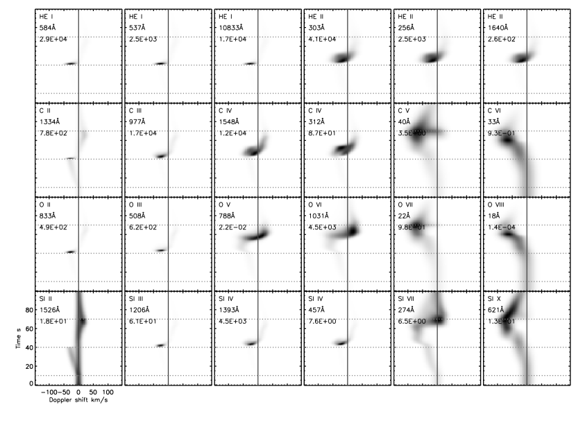
Figure 4: Spatially-averaged emission profiles from near the accelerated and heated footpoint of the loop, for calculation A. The emission was integrated along the vertical and averaged over all spatial positions within 2.175 Mm (corresponding to a 3 ″ spatial bin) of the footpoint in the low chromosphere. The panels are labeled with the atomic ion, central wavelength, and computed maximum total intensity ( ergs cm${}^{-2}\,$s${}^{-1}\,$sr^-1). The horizontal dotted lines demark the periods of acceleration and heating (10 to 40s), and of more intense heating (40 to 70s).

To compute profiles of selected EUV emission lines, we take the time-dependent populations of all ions of H, He, and of all charged ions of C, N, O, and Si¹⁺ through Si⁸⁺, and use these populations to compute the emitted power in selected lines, which are then integrated along a given line of sight to compute the line profiles assuming optically thin conditions. The same data are used in the calculation of radiative cooling for these ions. The approach of solving in time just for the ionization states of the ions, ignoring excited levels (except for the special case of hydrogen), is justified because for the ions of interest, the ion densities are accurately tracked in time and space and the emitted radiation can be computed post-facto because of the separation of timescales involved (Judge, 2005). We compute profiles using Gaussian profiles including both thermal and a 10  km s^-1 turbulent component to the line widths, and include the Doppler shifts of the moving plasma as seen vertically. To make meaningful comparisons with observations we average all the emission which, when observed vertically, lies within 2.175Mm (3″ as seen from earth) of the loop footpoint projected on the solar surface. This length was chosen simply because the “transition region” moves up and down significantly in our calculations (cf. Hansteen, 1993), and choosing a smaller length scales can produce artifacts as the transition region emission moves in and out of this range. (Also, the point spread functions of the best EUV spectrometers would have contributions wider than $1\arcsec$). Figure 4 shows the resulting line intensity profiles of a variety of lines of He, C, O and Si as a function of Doppler shift and time, for calculation A, in which additional heating and acceleration starts at $t=10$ sec. In each panel, the element, central wavelength and maximum (wavelength-integrated) intensities are listed. The figure shows profiles of lines with increasing atomic number, from top to bottom, and with increasing ionization stage- and hence typical formation temperature- from left to right. The intensities calculated generally exceed those measured in extant low-resolution observations, but given that the filling factor of type II spicules may be very small (e.g., de Pontieu et al., 2007), we do not consider this an important difference.

The overall dynamics is reflected in the lines of Si, from the chromospheric Si II 1526 Å line, through the Si X 621 Å coronal line. The upward acceleration of chromospheric plasma between 10 and 40s can be clearly traced in the calculations for the Si II line, and in the C II line. It is also visible in the coronal lines (C V, C IV, O VII, O VIII, Si X). But in these lines additional acceleration due to the pressure gradient in the hotter plasma extends for an additional 30 sec or so.

In fact the chromospheric and coronal lines behave quite differently: the blueshifts of the coronal lines are systematically larger than chromospheric and transition region lines by some 50-80  km s^-1 . The line profile of Si II for example shows chromospheric acceleration, but the blue-shifts disappear with the onset of the additional heating at $t=40s$. In contrast, the coronal lines are blueshifted relative to the Si II line when $t>40s$. After the forcing period the acoustic wave generated propagates away from the footpoint, and all the lines become dimmer. In addition, all chromospheric lines return near $t=100$s to zero Doppler shift and even become red-shifted (faintly seen in the lines of helium, for example).

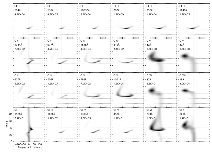
Figure 5: Same as Figure 4, but for calculation B, which has higher heating rates in denser plasma than calculation A, and shorter periods of heating and acceleration.

The different Doppler shifts calculated for chromospheric and coronal lines, found in this particular calculation, is a more general result. It is seen in calculation B, where the stronger heating rates produce sudden pressure-driven acceleration, so that the coronal line blueshifts exceed the Doppler shifts of chromospheric lines by $\sim 100$  km s^-1 (Figure 5). Several other calculations with different heating rates higher and lower in the chromosphere produce qualitatively similar results.

2.5 Other spectral signatures of the dynamics of heated outflowing plasma

Another systematic difference is seen in the emergent spectra we have calculated. The spectral lines we selected include some atomic transitions which have sensitivity to ionization non-equilibrium effects, through their relatively high excitation energy. Excitation of helium atoms and ions requires a large energy (compared with typical thermal energies found under ionization equilibrium conditions) because the excited levels have a larger principal quantum number $n$ than the ground levels. Any excitation requires a “$\Delta n\geq 1$” transition. In contrast, other atomic ions can have both $\Delta n=0$ and $\Delta n\geq 1$ transitions. The plotted 312 and 457 Å lines of C IV and Si IV respectively are $\Delta n=1$ transitions ($2s-3p$ and $3s-4p$), unlike the 1548 and 1393 Å lines which are $2s-2p$ and $3s-3p$ transitions respectively.

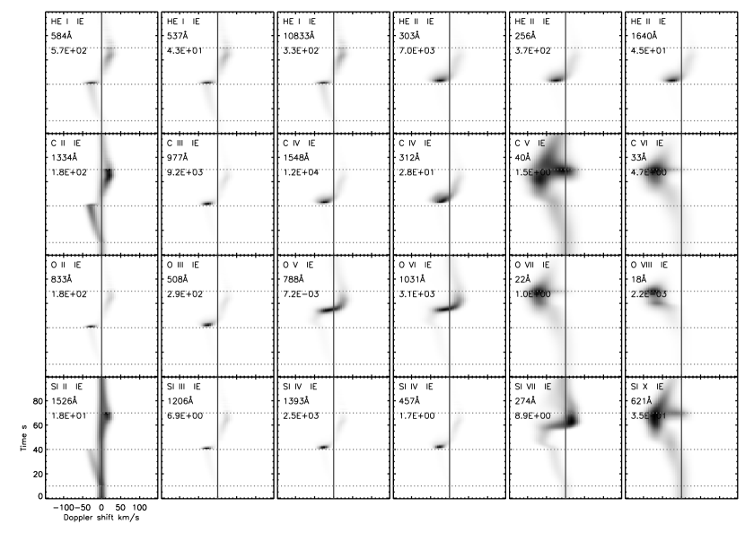
Figure 6: Same as Figure 4, but for calculations assuming instantaneous ionization equilibrium.

In Figure 6 we show the profiles computed with the full dynamics, but assuming instantaneous ionization equilibrium (IE). Comparison with Figure 4 clearly reveals departures from IE. The IE calculations are usually more variable as it takes some time for ions to become ionized or to recombine in response to changes in temperature and density. But, systematically, the $\Delta n=1$ transitions are all brighter than IE would predict. This effect results from plasma becoming ionized, under conditions where excitation and radiative decay of the levels occurs before the ion to which they belong becomes significantly ionized. In helium lines this has been invoked to explain their anomalous brightness (e.g. Jordan, 1975; Laming and Feldman, 1992; Pietarila and Judge, 2004; Judge and Pietarila, 2004; Judge, 2005). A similar effect is seen in the C IV and Si IV ions, but here we can compare directly the intensities $\Delta n=1$ with the $\Delta n=0$ transitions. In both cases, when the emitting plasma is undergoing heating, the $\Delta n=1$ transitions become enhanced relative to the $\Delta n=0$ transitions by a factor of 3.1 and 2.5 for Li-like C IV and Na-like Si IV respectively.

Such large departures from ionization equilibrium should be measurable. Simultaneous observations of the $\Delta n=0,1$ transitions in C IV and Si IV have presumably been obtained using the CDS and SUMER instruments on the SOHO spacecraft, but it is beyond the scope of the present paper to identify and analyze such data.

3 Discussion

Our 1D hydrodynamic calculations attempt to capture the evolution of the emitted spectrum of a plug of accelerated and heated plasma flowing along magnetic field lines extending upwards from the upper chromosphere. The dynamics and emergent spectra are computed using full non-equilibrium in the atomic rate equations. The calculations reveal that the coronal emission which accompanies the heating needed to produce coronal plasma from the cool spicular plasma is blueshifted by $\sim 50-90$  km s^-1 relative to the chromospheric emission (compare lines of He I, C II Si II with the coronal lines in figs. 4 5). This is because, in the hydrodynamic regime, the heating produces an over-pressure and a subsequent expansion of the plasma into the corona. Thus, if indeed the chromospheric plasma in Type II spicules is injected into the corona, at the same time being heated in this fashion, then we must expect the velocity distributions of chromospheric and coronal lines to differ. Accompanying the prediction of Doppler shift differences, changes in the intensities of line ratios that are traditionally viewed as being sensitive to electron temperature, are also predicted in our rapidly heated outflow models. These intensity changes result from the slowness of ionization/recombination processes relative to dynamical timescales. It would seem worthwhile to investigate atomic systems of the Li and Na-like isoelectronic sequences observationally, following earlier work (Heroux et al., 1972) as well as other atomic systems with temperature sensitive line ratios (e.g. Pinfield et al., 1999).

Such a systematic difference between cool and hot flows associated with Type II spicules has not been reported in the observational literature, but we note that the observations have significant uncertainties. The cool components of Type II spicules at the limb show apparent velocities of order 50-100  km s^-1 (de Pontieu et al., 2007), with rapid blueshifted events, thought be their disk counterparts, showing line-of-sight velocities of order 50  km s^-1 (Rouppe van der Voort et al., 2009) and apparent velocities of order 75  km s^-1 (De Pontieu et al., 2011). The velocities of coronal counterparts are also difficult to determine precisely. They are derived from weak blueshifted emission components, seen at the base of much stronger emission cores, near the limit at which EUV spectrographs can operate (e.g., instrumental broadening, signal-to-noise, …). These measurements suggest line-of-sight velocities of order 50-150  km s^-1 for the coronal counterparts of spicules. Because both the chromospheric and coronal measurements are significantly impacted by viewing geometry, radiative transfer and instrumental limitations, it is not yet clear that the observed velocity distributions are sufficiently well determined to reveal a velocity difference of 50  km s^-1 between the chromosphere and coronal counterparts of spicules.

If the large relative shift in the Doppler motions predicted here are not confirmed by future high resolution measurements (such as those from the IRIS mission), we would conclude that the suggestion put forward by de Pontieu et al. (2007); De Pontieu et al. (2009, 2011), namely the close correspondence of velocities from spicules with those of Doppler shifted lines in the transition region and corona, cannot credibly be accounted for in the type of 1D hydrodynamic flow modeled here. One possible resolution might simply be that the magnetic fields within the tube are significantly twisted such that the spicular plasma has an azimuthal as well as axial component as the Lorentz force directs the plasma along field lines. In this case the Doppler shifts computed should be multiplied by the cosine of the magnetic pitch angle.

The recent MHD calculations of Martínez-Sykora et al. (2011) might help resolve the problems identified here, in that the system modeled is far more complex than our simple calculations and does not seem to show such large velocity differences between chromospheric and coronal lines. In their work, they find that chromospheric material is injected into the corona via, first, compression due to horizontal Lorentz forces associated with emerging flux, and second, via the field-aligned gas pressure gradient. As the field-aligned flow progresses it is heated via Joule dissipation, in a fashion not dissimilar from the ad-hoc calculations we present. However, in the modeled MHD system, the acceleration and heating acts, with varying strength, on plasma that occurs on an ensemble of neighboring field lines. As a result, the coronal emission has contributions from many magnetic field lines with varying mixes of chromospheric and coronal plasma/flows. Thus, the line profiles of coronal plasma must be carefully synthesized to find the relative contributions of these different components. Notably though, the cool plasma that actually flows into the corona in these MHD calculations is indeed a field-aligned flow. Thus, if our parametrized heating and acceleration profiles are representative of what occurs in the complex 3D configuration, the heated plasma in that part of the calculated flow would be expected to behave like the calculations presented in the present paper. Current EUV observations lack the spatio-temporal resolution to resolve the finely structured dynamics and energetics predicted by the model of Martínez-Sykora et al. (2011).

The potential problem of Doppler shift differences may be avoided in an entirely different scenario (Judge et al., 2011), where it was suggested that Type II spicules, in particular those with apparent upward velocities in excess of 50  km s^-1, correspond not to jets but to the line-of-sight superposition of warped current sheets modulated by Alfvénic fluctuations driven from below. Low-frequency Alfvénic-type wave motions have been reported before in movies of Type II spicules (De Pontieu et al., 2007). Should Type II spicules be proven to be sheets, the calculations here are largely irrelevant, and the physical connection between the chromospheric, transition region and coronal emission proposed earlier would be called into question. But, as suggested by Judge et al. (2011) the 1D flow picture might apply to a subset of observed spicules with plasma genuinely flowing at lower speeds. However, several questions regarding the overall interpretation of spicule properties at the limb, their relation to RBEs, and statistical analyses would then arise.

Whatever the outcome, we conclude that the role of Type II spicules in supplying mass and energy to the corona (de Pontieu et al., 2007; De Pontieu et al., 2009, 2011), is a subject ripe for future study. Further observational work on spicule properties and their relationship to the properties of the associated hotter plasma seems warranted. The upcoming IRIS mission seems well positioned to address this question.

Appendix A Atomic rate equations

The system of equations integrated in time includes equations for the number densities of atoms and atomic ions. In 1D, these take the form

$${\partial~{}\over\partial t}n_{i}+{{\partial~{}\over\partial x}{vn_{i}}}=\sum^{N}_{j\neq i}n_{j}{}P_{ji}{}-n_{i}{}\sum^{N}_{j\neq i}P_{ij}{}.$$ (A1)

where $t,x$ are time and distance respectively, $n_{i}$ is the population density of atomic state $i$, and the coefficients $P_{ji}$ represent the transition rate, units s^-1, from state $j$ to state $i$ (and vice versa). Only long-lived states need tracking in time (Judge, 2005), so that the only states we solve for are the ground states of atomic ions and bare atomic nuclei. Given the solar radiation field and local thermal properties in the corona, the largest contributions to coefficients $P$ are ionization and recombination coefficients, by electron impact (charge transfer collisions with H and He are sometimes important but are not included here). Here we adopt the ionization rate coefficients of Arnaud and Rothenflug (1985), and fits to recombination rates in the form tabulated by Shull and Steenberg (1982), computed by one of us (PGJ) from the detailed photoionization cross sections computed by the OPACITY project (Seaton, 1987). These differ substantially from, and should be more accurate than, the calculations of (Shull and Steenberg, 1982). A comparison of recombination rates computed from the OPACITY project and more detailed work of Nahar and Pradhan (1992) is given in (Judge, 2007, Fig. 13). The systematic differences show the rates to agree within 0.2dex with some excursions of a factor of 2 possible.

Hydrogen ionization occurs not quite so simply as described above, and it is treated differently. This is because the $n=2$ levels can have a significant population owing to scattering in Ly$\alpha$ within the chromosphere, and Balmer continuum radiation from the upper photosphere can photoionize hydrogen (Hartmann and MacGregor, 1980; Vernazza et al., 1981, e.g.). Thus we include photoionization from the $n=2$ levels. We compute the $n=2$ populations assuming that Ly$\alpha$ is in detailed balance in the chromosphere (mostly neutral) but that the population is greatly reduced below this limit in the corona. As an ad-hoc, qualitative representation of these effects we apply the non-LTE factor $\left({n_{1}\over{n_{1}+n_{\kappa}}}\right)^{2}$:

$${n_{2}\over n_{1}}={n_{2}^{*}\over n_{1}^{*}}\left({n_{1}\over{n_{1}+n_{\kappa}}}\right)^{2}$$ (A2)

where the asterisk refers to LTE populations, and $n_{\kappa}$ is the population density of protons. We adopt a photoionization rate of $8\times 10^{3}$ s^-1 from the $n=2$ level (Vernazza et al., 1981). We assume radiative detailed balance throughout in the Lyman continuum and thus set photoionization and recombination rates to zero in that transition. This is not a serious problem in that it is correct in the chromosphere, and photoionization is not very important throughout the transition region and corona, relative to electron impact ionization.

Table 1: Parameters of the acceleration and heating

Calculation	$t_{1}$	$t_{2}$	$z_{1}$	$z_{2}$	$h_{1}$	$h_{2}$
	s	s	km	km
A	30	30	2000	2400	3	30
B	15	15	1900	2500	3	100

Note. — $t_{1}$ is the duration of the acceleration and moderate heating phase, $t_{2}$ the coasting and large heating phase. The initial atmospheric plasma between heights $z_{1}$ and $z_{2}$ is the region subject to the acceleration and heating. $h_{1}$ and $h_{2}$ measure the factors by which the nominal heating rates (equation 1) are increased during $t_{1}$ and $t_{2}$ respectively.

Figure 1: The initial, near-equilibrium state of the atmosphere is shown.

Figure 2: The state of the atmosphere after 20 seconds of acceleration and moderate extra heating in the upper chromosphere is shown, for calculation A.

Figure 3: The state of the atmosphere 20 seconds into the intense heating phase is shown, for calculation A.

References

- Arnaud and Rothenflug (1985) Arnaud, M. and Rothenflug, R.: 1985, Astron. Astrophys. Suppl. Ser. 60, 425
- Aschwanden et al. (2007) Aschwanden, M. J., Winebarger, A., Tsiklauri, D., and Peter, H.: 2007, Astrophys. J. 659, 1673
- Athay (1986) Athay, R. G.: 1986, Astrophys. J. 308, 975
- Athay and Holzer (1982) Athay, R. G. and Holzer, T.: 1982, Astrophys. J. 255, 743
- Beckers (1968) Beckers, J. M.: 1968, Solar Phys. 3, 367
- Beckers (1972) Beckers, J. M.: 1972, Ann. Rev. Astron. Astrophys. 10, 73
- Carlsson and Stein (1995) Carlsson, M. and Stein, R. F.: 1995, Astrophys. J. 440, L29
- de Pontieu et al. (2007) de Pontieu, B., McIntosh, S., Hansteen, V. H., Carlsson, M., Schrijver, C. J., Tarbell, T. D., Title, A. M., Shine, R. A., Suematsu, Y., Tsuneta, S., Katsukawa, Y., Ichimoto, K., Shimizu, T., and Nagata, S.: 2007, Publ. Astron. Soc. Japan 59, 655
- De Pontieu et al. (2011) De Pontieu, B., McIntosh, S. W., Carlsson, M., Hansteen, V. H., Tarbell, T. D., Boerner, P., Martinez-Sykora, J., Schrijver, C. J., and Title, A. M.: 2011, Science 331, 55
- De Pontieu et al. (2007) De Pontieu, B., McIntosh, S. W., Carlsson, M., Hansteen, V. H., Tarbell, T. D., Schrijver, C. J., Title, A. M., Shine, R. A., Tsuneta, S., Katsukawa, Y., Ichimoto, K., Suematsu, Y., Shimizu, T., and Nagata, S.: 2007, Science 318, 1574
- De Pontieu et al. (2009) De Pontieu, B., McIntosh, S. W., Hansteen, V. H., and Schrijver, C. J.: 2009, Astrophys. J. Lett. 701, L1
- Goodman (2004) Goodman, M. L.: 2004, Astron. Astrophys. 416, 1159
- Hansteen (1993) Hansteen, V.: 1993, Astrophys. J. 402, 741
- Hansteen et al. (2010) Hansteen, V. H., Hara, H., De Pontieu, B., and Carlsson, M.: 2010, ApJ 718, 1070
- Hartmann and MacGregor (1980) Hartmann, L. and MacGregor, K. B.: 1980, Astrophys. J. 242, 260
- Heroux et al. (1972) Heroux, L., Cohen, M., and Malinovsky, M.: 1972, Solar Phys. 23, 369
- Jordan (1975) Jordan, C.: 1975, Mon. Not. R. Astron. Soc. 170, 429
- Judge (2007) Judge, P.: 2007, THE HAO SPECTRAL DIAGNOSTIC PACKAGE FOR EMITTED RADIATION (haos-diper) Reference Guide (Version 1.0), Technical Report NCAR/TN-473-STR, National Center for Atmospheric Research
- Judge (2005) Judge, P. G.: 2005, J. Quant. Spectrosc. Radiat. Transfer 92(4), 479
- Judge and Pietarila (2004) Judge, P. G. and Pietarila, A.: 2004, Astrophys. J. 606, 1258
- Judge et al. (2011) Judge, P. G., Tritschler, A., and Low, B. C.: 2011, ApJ 730, L4
- Kosugi et al. (2007) Kosugi, T., Matsuzaki, K., Sakao, T., Shimizu, T., Sone, Y., Tachikawa, S., Hashimoto, T., Minesugi, K., Ohnishi, A., Yamada, T., Tsuneta, S., Hara, H., Ichimoto, K., Suematsu, Y., Shimojo, M., Watanabe, T., Shimada, S., Davis, J. M., Hill, L. D., Owens, J. K., Title, A. M., Culhane, J. L., Harra, L. K., Doschek, G. A., and Golub, L.: 2007, Solar Phys. 243, 3
- Kuperus et al. (1981) Kuperus, M., Ionson, J. A., and Spicer, D. S.: 1981, Ann. Rev. Astron. Astrophys. 19, 7
- Laming and Feldman (1992) Laming, J. M. and Feldman, U.: 1992, Astrophys. J. 386, 364
- Landi et al. (2006) Landi, E., Del Zanna, G., Young, P. R., Dere, K. P., Mason, H. E., and Landini, M.: 2006, Astrophys. J. Suppl. Ser. 162, 261
- Mariska (1992) Mariska, J. T.: 1992, The Solar Transition Region, Cambridge Univ. Press, Cambridge UK
- Martínez-Sykora et al. (2011) Martínez-Sykora, J., De Pontieu, B., Hansteen, V., and McIntosh, S. W.: 2011, Astrophys. J. 732, 84
- McIntosh and De Pontieu (2009) McIntosh, S. W. and De Pontieu, B.: 2009, Astrophys. J. 706, L80
- McIntosh et al. (2010) McIntosh, S. W., Innes, D. E., de Pontieu, B., and Leamon, R. J.: 2010, Astron. Astrophys. 510, L2
- Miyamoto (1949) Miyamoto, S.: 1949, Publ. Astron. Soc. Japan 1, 14
- Nahar and Pradhan (1992) Nahar, S. and Pradhan, A. K.: 1992, Phys. Rev. Lett. 68, 1488
- Parker (1994) Parker, E. N.: 1994, Spontaneous Current Sheets in Magnetic Fields with Application to Stellar X-Rays, International Series on Astronomy and Astrophyics, Oxford University Press, Oxford
- Pietarila and Judge (2004) Pietarila, A. and Judge, P. G.: 2004, Astrophys. J. 606, 1239
- Pinfield et al. (1999) Pinfield, D. J., Keenan, F. P., Mathioudakis, M., Phillips, K. J. H., Curdt, W., and Wilhelm, K.: 1999, Astrophys. J. 527, 1000
- Pneuman and Kopp (1978) Pneuman, G. and Kopp, R.: 1978, Sol. Phys. 57, 49
- Raymond and Smith (1977) Raymond, J. C. and Smith, B. W.: 1977, Astrophys. J. Suppl. Ser. 35, 419
- Roberts (1945) Roberts, W. O.: 1945, Astrophys. J. 101, 136
- Rouppe van der Voort et al. (2009) Rouppe van der Voort, L., Leenaarts, J., de Pontieu, B., Carlsson, M., and Vissers, G.: 2009, Astrophys. J. 705, 272
- Seaton (1987) Seaton, M. J.: 1987, J. Phys. B: At. Mol. Phys. 20, 6363
- Shull and Steenberg (1982) Shull, J. M. and Steenberg, M. V.: 1982, Astrophys. J. Suppl. Ser. 48, 95
- Sterling (2000) Sterling, A. C.: 2000, Solar Phys. 196, 79
- Thomas (1948) Thomas, R. N.: 1948, Astrophys. J. 108, 130
- Tsuneta et al. (2008) Tsuneta, S., Ichimoto, K., Katsukawa, Y., Nagata, S., Otsubo, M., Shimizu, T., Suematsu, Y., Nakagiri, M., Noguchi, M., Tarbell, T., Title, A., Shine, R., Rosenberg, W., Hoffmann, C., Jurcevich, B., Kushner, G., Levay, M., Lites, B., Elmore, D., Matsushita, T., Kawaguchi, N., Saito, H., Mikami, I., Hill, L. D., and Owens, J. K.: 2008, Solar Phys. 249, 167
- Vernazza et al. (1981) Vernazza, J., Avrett, E., and Loeser, R.: 1981, Astrophys. J. Suppl. Ser. 45, 635
- Walsh and Ireland (2003) Walsh, R. W. and Ireland, J.: 2003, Astron. Astrophys. 12, 1