Two-body Coulomb scattering and complex scaling

Abstract

The two-body Coulomb scattering problem is solved using the standard complex scaling method. The explicit enforcement of the scattering boundary condition is avoided. Splitting of the scattering wave function based on the Coulomb modified plane wave is considered. This decomposition leads a three-dimensional Schrödinger equation with source term. Partial wave expansion is carried out and the asymptotic form of the solution is determined. This splitting does not lead to simplification of the scattering boundary condition if complex scaling is invoked. A new splitting carried out only on partial wave level is introduced and this method is proved to be very useful. The scattered part of the wave function tends to zero at large inter-particle distance. This property permits of easy numerical solution: the scattered part of the wave function can be expanded on bound-state type basis. The new method can be applied not only for pure Coulomb potential but in the presence of short range interaction too.

I Introduction

The method of complex scaling (CS) has been an excellent tool to calculate half life times of resonance states for a long time. The CS has been successfully applied in many areas of quantum physics ho83 ; moi98 and it has been extended to collision processes very early on nut69 ; hen72 . However, a drawback of the standard CS (or the uniform CS) has emerged immediately after the introduction of the method. For scattering problems the CS procedure can be applied only for short range potentials nut69 ; bau75 . This is indeed serious since the long range Coulomb interaction can not be neglected in majority of the problems of atomic and nuclear physics. Several modifications have been suggested joh84 ; res85 ; pes92 but none of them has reached a widespread acceptance. After these initial applications the scattering aspects of the CS has been neglected.

The turning point has been the work res97 where it has been shown that scattering calculations with the exterior CS can be successfully performed for long range interactions. After this pioneering work the exterior CS method has been applied for variety of three-body Coulomb problems, even above the three-body breakup threshold, with great success bar06 ; cur04a ; cur04b ; bae01 . The exterior CS method has proved to be one of the most successful numerical methods to deal with collision processes. However, recently the exterior CS method has been under scrutiny since in the method an artificial cutoff in some of the interaction is used. To solve this problem a modification of the original exterior CS method has been suggested and checked in two-body calculations Vol09 ; Yak10 . Extension to three-body problem has been also sketched Ela09 .

Recently it has been shown kru07 that the standard CS can be applied for scattering problems when a short range potential is added to the pure Coulomb interaction. The method is based on the two potential formalism. Similar approach has been suggested also in cur04 . In the present paper we rigorously develop a method which is equally good for pure Coulomb interaction and for the general case too (i.e. a short range potential is added to the Coulomb interaction). The new approach does not rely on the two potential formalism and dangerous cutoff will not be introduced.

In the case of a two-body problem the wave function depends on the inter-particle coordinate ${\bf r}$. The scattering solution of the Schrödinger equation with momentum ${\bf k}$ is denoted by $\psi^{+}({\bf k},{\bf r})$. This wave function will be called three dimensional (3D) wave function. It is assumed that the wave function satisfies appropriate scattering boundary conditions. The aim of the application of any CS method is to introduce a new equation instead of the Schrödinger equation with simplified boundary conditions. The expectation is that the solution of this new equation is square integrable therefore it can be approximated by bound-state type basis functions. In this way the explicit use of the complicated scattering asymptotic form of the wave function can be avoided and the numerical calculation can be simplified.

In contrast to resonance state calculation in scattering problem the CS is not applied directly to the full wave function. First a splitting of the total wave function is carried out. The full scattering solution is searched in the form

$$\psi^{+}({\bf k},{\bf r})=\phi_{0}({\bf k},{\bf r})+\psi^{sc+}({\bf k},{\bf r}),$$ (1)

where $\phi_{0}({\bf k},{\bf r})$ is a known function. From the Schrödinger equation for the scattered part of the wave function the so called driven Schrödinger equation (or Schrödinger equation with source)

$$(E-\hat{H})\psi^{sc+}({\bf k},{\bf r})=S({\bf k},{\bf r}),$$ (2)

can be derived. The source term is given by $S({\bf k},{\bf r})=(\hat{H}-E)\phi_{0}({\bf k},{\bf r}).$ The Hamiltonian and energy are denoted by $\hat{H}$ and $E$ respectively.

We mention that the two-body Coulomb problem with source has been recently thoroughly investigated in Gas10 . Complicated but exact solutions have been given for very general sources. Basis functions with proper two-body scattering asymptotic have been generated from the exact solutions and used in the J-matrix method Anc11 . The driven Schrödinger equation has been applied for realistic three-body scattering problems too ran11 ; fra10 . However, in these works CS has not been applied and the complicated scattering boundary conditions have been implemented using either the finite element method or Sturmian expansion.

The CS in scattering calculations means that the coordinate ${\bf r}$ in Eq. (2) is replaced by ${\bf r}e^{i\theta}$ where $0<\theta<\pi/2$. The boundary condition is simplified if after complex scaling the scattered part of the wave function goes to zero when the inter-particle distance tends to infinity. It is easy too see that this property is fulfilled if $\psi^{sc+}({\bf k},{\bf r})$ contains only outgoing spherical wave. In the paper this property will be investigated for different splittings of the full wave function.

The organization of the paper is the following. In section II the known expressions of the two-body Coulomb scattering are reviewed. The driven Schrödinger equation is introduced in section III. The splitting of the total wave function in Eq. (1) is carried out on 3D level, however, the splitting can be carried out only on partial wave (p.w.) level. Different 3D and p.w. splittings will be considered and it will be shown that there are cases when the 3D and p.w. splittings are not equivalent. The Coulomb modified plane wave (CMPW) plays a basic role in the recent surface integral formalism of the scattering theory Kad09 ; Kad05 . The properties of the 3D splitting based on the CMPW will be investigated in section IV. A useful p.w. splitting from the point of view of the CS will be introduced in section V. Finally numerical examples will be presented both for the pure Coulomb case and for a potential having short and long range parts. The conclusions will be given in section VII.

II Exact solutions of the two-body Coulomb problem

First we collect a few known expressions har for the two-body Coulomb scattering in order to fix the notations. As usual we take $\hbar=m=e=1$ (m is the reduced mass), the energy is $E=k^{2}/2>0$ and the Coulomb-potential reads $\gamma k/r$, where $\gamma$ is the Sommerfeld-parameter. We consider the Schrödinger equation with pure two-body Coulomb interaction

$$\left(-\frac{1}{2}\Delta_{{\bf r}}+\frac{\gamma k}{r}-\frac{k^{2}}{2}\right)\psi({\bf k},{\bf r})=0,$$ (3)

where $\Delta_{{\bf r}}$ is the Laplace-operator. The Coulomb scattering state

$$\psi_{c}^{+}({\bf k},{\bf r})=e^{-\pi\gamma/2}\Gamma(1+i\gamma)e^{i{\bf k}{\bf r}}M(-i\gamma,1,ikr-i{\bf k}{\bf r})$$ (4)

is a solution of (3). Here $M(a,b,z)$ is the regular confluent hypergeometric function abra . The partial wave expansion is given by the well known form

$$\psi_{c}^{+}({\bf k},{\bf r})=\sum_{l=0}^{\infty}(2l+1)\psi^{+}_{l}(k,r)P_{l}(\cos\vartheta),$$ (5)

where $P_{l}(z)$ is the Legendre polynomial and $\vartheta$ is the angle between the vectors ${\bf k}$ and ${\bf r}$. The full radial part $\psi^{+}_{l}(k,r)$ is expressed with the help of the regular Coulomb function $F_{l}(k,r)$

$$\psi^{+}_{l}(k,r)=\frac{1}{kr}i^{l}\exp(i\sigma_{l})F_{l}(k,r).$$ (6)

The explicit formula reads

$$\psi^{+}_{l}(k,r)=\frac{\Gamma(l+1+i\gamma)}{\Gamma(2l+2)}e^{-\gamma\pi/2}e^{-ikr}(2ikr)^{l}M(l+1-i\gamma,2l+2,2ikr)$$ (7)

and the Coulomb phase shift is defined by $e^{2i\sigma_{l}}=\Gamma(l+1+i\gamma)/\Gamma(l+1-i\gamma)$. The p.w. components $\psi^{+}_{l}(k,r)$ satisfy the radial Schrödinger equation

$$\left[-\frac{1}{2r}\frac{d^{2}}{dr^{2}}r+\frac{l(l+1)}{2r^{2}}+\frac{\gamma k}{r}-\frac{k^{2}}{2}\right]\psi_{l}(k,r)=0.$$ (8)

The Coulomb scattering function can be split into so called incoming and scattered waves har2 . Using the identity 7.2.2.9 in prud we can write

$$\psi_{c}^{+}({\bf k},{\bf r})=\psi_{i}({\bf k},{\bf r})+\psi_{s}({\bf k},{\bf r}),$$ (9)

where

$$\psi_{i}({\bf k},{\bf r})=e^{\pi\gamma/2}e^{i{\bf k}{\bf r}}U(-i\gamma,1,ikr-i{\bf k}{\bf r}),$$ (10)

and

$$\psi_{s}({\bf k},{\bf r})=e^{\pi\gamma/2}\frac{\Gamma(1+i\gamma)}{\Gamma(-i\gamma)}e^{ikr}U(1+i\gamma,1,i{\bf k}{\bf r}-ikr).$$ (11)

The notation $U(a,b,z)$ stands for the irregular confluent hypergeometric function abra . Interestingly not only $\psi_{c}^{+}({\bf k},{\bf r})$ but the functions $\psi_{i}({\bf k},{\bf r})$ and $\psi_{s}({\bf k},{\bf r})$ satisfy the 3D Scrödinger equation (3).

The partial wave expansions of the incoming and scattered parts are given in har2 . Later we will use them so we quote the main result of paper har2 . We use a very similar notation as in har2 however we have rewritten the Whittaker function $W$ in terms of $U$.

The p.w. expansions of $\psi_{i}({\bf k},{\bf r})$ and $\psi_{s}({\bf k},{\bf r})$ are given in the same form as (5) but the p.w. components now read

$$\psi_{i,l}(k,r)=\omega_{i,l}(k,r)+\chi_{l}(k,r)$$ (12)

and

$$\psi_{s,l}(k,r)=\omega_{s,l}(k,r)-\chi_{l}(k,r).$$ (13)

We note that our definitions of $\omega_{i,l}$, $\omega_{s,l}$ and $\chi_{l}$ are constant times of the original ones har2 . The explicit expressions are the followings

$$\omega_{i,l}(k,r)=e^{-ikr}e^{\gamma\pi/2}(-1)^{l+1}(2ikr)^{l}U(l+1-i\gamma,2l+2,2ikr),$$ (14)

$$\omega_{s,l}(k,r)=e^{ikr}e^{2i\sigma_{l}+\gamma\pi/2}(-1)^{l+1}(2ikr)^{l}U(l+1+i\gamma,2l+2,-2ikr)$$ (15)

and

$$\chi_{l}(k,r)=\frac{e^{ikr+\gamma\pi/2}}{2ikr}\frac{(-1)^{l}}{(2ikr)^{l}}\frac{\Gamma(2l+1)}{\Gamma(l+1-i\gamma)}\sum_{n=0}^{l}\frac{(-1)^{n}(i\gamma-l)_{n}}{(-2l)_{n}n!}(2ikr)^{n}.$$ (16)

The equation

$$\psi^{+}_{l}(k,r)=\omega_{i,l}(k,r)+\omega_{s,l}(k,r)$$ (17)

is also proved in har2 . We mention that the splitting (17) simply follows from (7) if the function $M(l+1-i\gamma,2l+2,2ikr)$ is rewritten in terms of the irregular confluent hypergeometric functions U using the equation 7.2.2.9 of prud .

Although the functions $\psi_{i}({\bf k},{\bf r})$ and $\psi_{s}({\bf k},{\bf r})$ are solutions of the 3D Schrödinger equation (3) surprisingly its partial wave components $\psi_{i,l}(k,r)$ and $\psi_{s,l}(k,r)$ do not satisfy the radial Schrödinger equation (8) (for details see har2 ). This property will be proved to be very important for our new method.

Using the asymptotic expansion 13.5.2 of abra we get the asymptotic form of the Coulomb-scattering wave function in the well known form

$$\psi_{c}^{+}({\bf k},{\bf r})=e^{i{\bf k}{\bf r}}(kr-{\bf k}{\bf r})^{i\gamma}\left[1+O\left(\frac{1}{kr}\right)\right]+f_{c}(\cos(\vartheta))\frac{e^{ikr-i\gamma\ln(2kr)}}{r}\left[1+O\left(\frac{1}{kr}\right)\right],$$ (18)

where $f_{c}(\cos(\vartheta))$ is the Coulomb scattering amplitude. The function $e^{i{\bf k}{\bf r}}(kr-{\bf k}{\bf r})^{i\gamma}$ is called CMPW.

III Driven Scrödinger equation

The scattering solution of the Scrödinger equation is searched in the form (1). From the Scrödinger equation (3) with a simple rearrangement the following driven Schrödinger equation (or Scrödinger equation with source)

$$\left(\frac{p^{2}}{2}+\frac{1}{2}\Delta_{{\bf r}}-\frac{\gamma k}{r}\right)\psi^{sc+}({\bf k},{\bf r})=S({\bf k},{\bf r}),$$ (19)

can be derived for $\psi_{c}^{sc+}({\bf k},{\bf r})$. The source term is given by

$$S({\bf k},{\bf r})=\left(-\frac{1}{2}\Delta_{{\bf r}}+\frac{\gamma k}{r}-\frac{k^{2}}{2}\right)\phi_{0}({\bf k},{\bf r}).$$ (20)

We mention that the driven Scrödinger equation (19) has been studied in Gas10 . For quite general sources very complicated analytic solutions can be found Gas10 . The aim of our paper is to derive an easy numerical method to solve (19) and from the scattered part of the wave function deduce the scattering amplitude.

The asymptotic form (18) inspires the following choice for $\phi_{0}({\bf k},{\bf r})$

$$\phi_{0}({\bf k},{\bf r})=e^{i{\bf k}{\bf r}}(kr-{\bf k}{\bf r})^{i\gamma}.$$ (21)

This splitting is based on the CMPW and it has been used in Kad09 ; Kad05 in order to derive the surface integral formalism of the scattering theory. Using Descartes-coordinates it is easy to derive a simple form for the source term

$$S({\bf k},{\bf r})=\frac{\gamma^{2}k}{r(kr-{\bf k}{\bf r})}e^{i{\bf k}{\bf r}}(kr-{\bf k}{\bf r})^{i\gamma}.$$ (22)

We may try to use the splitting based in the incoming Coulomb wave function i.e. we make the following choice

$$\phi_{0}({\bf k},{\bf r})=\psi_{i}({\bf k},{\bf r})$$ (23)

instead of (21). In this case we get $S({\bf k},{\bf r})=0$. This follows from the fact the function $\psi_{i}({\bf k},{\bf r})$ satisfies (3). In this case we do not get a driven Schrödinger equation, $\psi^{sc+}({\bf k},{\bf r})$ satisfies the original homogeneous equation (3) and $\psi^{sc+}({\bf k},{\bf r})=\psi_{s}({\bf k},{\bf r})$.

If we want to derive the p.w. form of the driven Scrödinger equation (19) we have to have the p.w. expansions of the source term

$$S({\bf k},{\bf r})=\sum_{l=0}^{\infty}(2l+1)S_{l}(k,r)P_{l}(\cos(\vartheta))$$ (24)

and of $\phi_{0}({\bf k},{\bf r})$

$$\phi_{0}({\bf k},{\bf r})=\sum_{l=0}^{\infty}(2l+1)\phi_{0,l}(k,r)P_{l}(\cos(\vartheta)).$$ (25)

Using the operator identity mes

$$\Delta_{{\bf r}}=\frac{1}{r}\frac{d^{2}}{dr^{2}}r-\frac{\hat{L}^{2}}{r^{2}},$$ (26)

where $\hat{L}^{2}$ is the square of the orbital angular momentum operator, we can derive the partial wave form of the driven Schrödinger equation (19)

$$\left[\frac{k^{2}}{2}+\frac{1}{2r}\frac{d^{2}}{dr^{2}}r-\frac{l(l+1)}{2r^{2}}-\frac{\gamma k}{r}\right]\psi_{l}^{sc+}(k,r)=S_{l}(k,r),$$ (27)

where

$$\psi^{sc+}({\bf k},{\bf r})=\sum_{l=0}^{\infty}(2l+1)\psi^{sc+}_{l}(k,r)P_{l}(\cos(\vartheta)).$$ (28)

Later it will be proved to be very useful if we make the splitting of the scattering wave function not in the 3D form (1) but on the p.w. level. We take the p.w. component of the scattering wave function in the following form

$$\psi_{l}^{+}(k,r)=\tilde{\phi}_{0,l}(k,r)+\tilde{\psi}_{l}^{sc+}(k,r),$$ (29)

where $\tilde{\phi}_{0,l}(k,r)$ is a fixed known function and $\tilde{\psi}_{l}^{sc+}(k,r)$ is considered as an unknown function. From the partial wave Schrödinger equation we get the following non-homogeneous differential equation

$$\left[\frac{k^{2}}{2}+\frac{1}{2r}\frac{d^{2}}{dr^{2}}r-\frac{l(l+1)}{2r^{2}}-\frac{\gamma k}{r}\right]\tilde{\psi}_{l}^{sc+}(k,r)=\tilde{S}_{l}(k,r)$$ (30)

where

$$\tilde{S}_{l}(k,r)=\left[-\frac{1}{2r}\frac{d^{2}}{dr^{2}}r+\frac{l(l+1)}{2r^{2}}+\frac{\gamma k}{r}-\frac{k^{2}}{2}\right]\tilde{\phi}_{0,l}(k,r).$$ (31)

If we take $\tilde{\phi}_{0,l}(k,r)$ identical to the partial wave component of $\phi_{0}({\bf k},{\bf r})$ i.e. $\tilde{\phi}_{0,l}(k,r)=\phi_{0,l}(k,r)$ then the source terms $S_{l}(k,r)$ and $\tilde{S}_{l}(k,r)$ are identical if in equation (20) the action of the Laplace-operator can be given in the form (26). This replacement however is valid only for those functions which are finite at $r=0$ (see page 496 mes ).

In the case of splitting based on (23) the function $\psi_{i}({\bf k},{\bf r})$ is not finite at $r=0$. In this circumstance the 3D splitting and the p.w. level splitting are different. We have already seen that the 3D splitting based on (23) does not lead to a driven Schrödinger equation. However if we make the following p.w. splitting

$$\psi_{l}^{+}(k,r)=\psi_{i,l}(k,r)+\tilde{\psi}_{l}^{sc+}(k,r),$$ (32)

i.e we take $\tilde{\phi}_{0,l}(k,r)=\psi_{i,l}(k,r)$ then we get a driven radial Schrödinger equation. Direct calculation of (31) gives the following source term

$$\tilde{S}_{l}(k,r)=\frac{e^{ikr+\gamma\pi/2}}{2r^{2}\Gamma(-i\gamma)}.$$ (33)

Interestingly the source term is independent from $l$. The derivation of (33) is given in Appendix A.

IV Partial wave expansion and asymptotic forms

The p.w. expansion of $\psi_{i}({\bf k},{\bf r})$ is given in har2 and we have reviewed it earlier. We now determine the corresponding expansion of the CMPW. The p.w. expansion of the CMPW is written in the standard form

$$e^{i{\bf k}{\bf r}}(kr-{\bf k}{\bf r})^{i\gamma}=\sum_{l=0}^{\infty}(2l+1)\tau_{l}(k,r)P_{l}(\cos(\vartheta)).$$ (34)

and the radial functions are given by the integral

$$\tau_{l}(k,r)=\frac{1}{2}(kr)^{i\gamma}\int_{-1}^{1}e^{ikrx}(1-x)^{i\gamma}P_{l}(x)dx.$$ (35)

A compact expression for the p.w. component of the CMPW can be given for arbitrary $l$. Using (35) and the integral 2.17.5.6 in prud we get

$$\tau_{l}(k,r)=\frac{(-i\gamma)_{l}}{(1+i\gamma)_{l+1}}(2kr)^{i\gamma}e^{ikr}\ _{2}F_{2}(1+i\gamma,1+i\gamma;l+2+i\gamma,1+i\gamma-l;-2ikr),$$ (36)

where $(a)_{n}$ is the Pochhammer symbol.

For the application of the complex scaling we have to know the asymptotic behavior of the scattered part of the wave function $\psi_{l}^{sc+}(k,r)$. Here we derive formulas valid at large $r$ values. With the help of the expression 13.5.2 abra we get the following asymptotic expansions valid at $r\rightarrow\infty$

$$\omega_{i,l}(k,r)\sim\frac{e^{-ikr}(2kr)^{i\gamma}}{2ikr}(-1)^{l+1}\sum_{n=0}^{\infty}a_{i,n}^{l}\frac{1}{(2ikr)^{n}}$$ (37)

and

$$\omega_{s,l}(k,r)\sim\frac{e^{ikr}(2kr)^{-i\gamma}}{2ikr}e^{2i\sigma_{l}}\sum_{n=0}^{\infty}a_{s,n}^{l}\frac{1}{(2ikr)^{n}}.$$ (38)

The expansion coefficients are given by $a_{i,n}^{l}=(-1)^{n}(l+1-i\gamma)_{n}(-l-i\gamma)_{n}/n!$ and $a_{s,n}^{l}=(l+1+i\gamma)_{n}(-l+i\gamma)_{n}/n!$. These asymptotic forms show that with the help of the splitting (17) the incoming and outgoing spherical waves are clearly separated in the p.w. Coulomb-scattering wave function.

In order to derive an asymptotic expansion of $\tau_{l}(k,r)$ we express (36) in terms of Meijer’s $G$ function. Using 5.11.1(2) luke we get

$$\tau_{l}(k,r)=e^{ikr}(2kr)^{i\gamma}(-1)^{l}G_{2,3}^{1,2}\left(2ikr\left|\begin{array}[]{ccc}-i\gamma,&-i\gamma\\ 0,&-1-i\gamma-l,&l-i\gamma\end{array}\right.\right).$$ (39)

We are interested in the asymptotic behavior after the CS is carried out i.e. $r$ is replaced by $re^{i\theta}$ and $0<\theta<\pi$. We give the asymptotic expansion valid in this case. Considering the expression 6.5.32 abra we can derive

$$\tau_{l}(k,re^{i\theta})\sim\frac{e^{-ikre^{i\theta}}}{2ikre^{i\theta}}(2kre^{i\theta})^{i\gamma}(-1)^{l+1}\sum_{n=0}^{\infty}\frac{d^{l}_{n}(-2)^{n}}{(2ikre^{i\theta})^{n}},$$ (40)

where the expansion coefficients satisfy the recursion

$$4(n+1)d^{l}_{n+1}=2[2n^{2}-n(2i\gamma-1)-l^{2}-l-i\gamma]d^{l}_{n}-n(n-l-i\gamma-1)(n+l-i\gamma)d^{l}_{n-1}$$ (41)

and $d^{l}_{0}=1$.

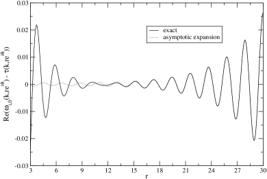
Figure 1: The function $\omega_{i,0}(k,r)-\tau_{0}(k,r)$ and the next to leading order term of its asymptotic expansion (44) are complex scaled using $\theta=0.1$. Only the real parts are displayed. The momentum is $k=3$, the Sommerfeld-parameter $\gamma=1/3$ and $l=0$. The solid line denotes the exact values and the dashed line corresponds to the asymptotic expansion (44).

Since the p.w. components are related to each other by the simple relation

$$\psi_{l}^{+}(k,r)=\tau_{l}(k,r)+\psi_{l}^{sc+}(k,r)$$ (42)

and we have the splitting (17) we can write

$$\psi_{l}^{sc+}(k,r)=\left[\omega_{i,l}(k,r)-\tau_{l}(k,r)\right]+\omega_{s,l}(k,r).$$ (43)

We notice that the last term in (43) $\omega_{s,l}(k,r)$ asymptotically contains only outgoing spherical wave (see Eq. (38)) so the applicability of the CS is determined by the behavior of $\omega_{i,l}(k,re^{i\theta}))-\tau_{l}(k,re^{i\theta}))$ at $r\rightarrow\infty$. Fortunately the asymptotic expansions of the functions $\omega_{i,l}(k,r)$ and $\tau_{l}(k,r)$ are carried out using the same asymptotic sequence of functions $\{e^{-ikr}(2kr)^{i\gamma}(-1)^{l+1}/(2ikr)^{n},\ n=0,1,2\ldots\}$ so we can simply add/subtract the asymptotic expansions as required erdelyi . Using (37) and (40) we can write down the following asymptotic expansion

$$\left[\omega_{i,l}(k,re^{i\theta})-\tau_{l}(k,re^{i\theta})\right]\sim\frac{e^{-ikre^{i\theta}}}{2ikre^{i\theta}}(2kre^{i\theta})^{i\gamma}(-1)^{l+1}\sum_{n=0}^{\infty}\frac{a_{i,n}^{l}-d^{l}_{n}(-2)^{n}}{(2ikre^{i\theta})^{n}}.$$ (44)

Let’s investigate (44). We realize that $a_{i,0}^{l}-d^{l}_{0}=0$. This means that in leading order $\psi_{l}^{sc+}(k,re^{i\theta})$ does not contain complex scaled incoming spherical wave. However in higher orders $\psi_{l}^{sc+}(k,re^{i\theta})$ do contains complex scaled ”generalized” incoming spherical wave ($e^{-ikr}/r^{n}$, $n>1$). This means that the complex scaled scattered part of the wave function $\psi_{l}^{sc+}(k,re^{i\theta})$ does not tend zero as $r\rightarrow\infty$.

This finding is demonstrated in Fig. 1. Both the left hand side and the right hand side of (44) are displayed. From the asymptotic expansion only the next to leading order term is considered (the leading order term is zero). The real part of the function $\omega_{i,0}(k,re^{i\theta})-\tau_{0}(k,re^{i\theta})$ first starts to oscillate with decreasing order of amplitude however at larger $r$ values the presence of the terms of the form $e^{-ikre^{i\theta}}/(re^{i\theta})^{n}$ dominate and the amplitude of the oscillation becomes larger and larger.

We have got a very unfortunate result, if we use the 3D splitting based on the CMPW then the scattered part of the wave function asymptotically contains both incoming and outgoing spherical waves. This fact prevents the application of the complex scaling.

V Complex scaling and scattering states

In the previous section we have established that the splitting of the wave function based on the CMPW i.e. the choice (21) is useless from the point of view of CS. Now we turn to the splitting (32) which is carried out on the p.w. level. The scattered part of the wave function is given by

$$\tilde{\psi}_{l}^{sc+}(k,r)=\omega_{s,l}(k,r)-\chi_{l}(k,r).$$ (45)

This equation follows from (12), (17) and (32). The asymptotic form (38) and the expression (16) for $\chi_{l}(k,r)$ shows that the scattered part of the wave function now contains only outgoing spherical wave and so the complex scaling can be safely applied. From (16) and (38) we get in leading order

$$\tilde{\psi}_{l}^{sc+}(k,r) = e^{2i\sigma_{l}}\frac{e^{ikr}(2kr)^{-i\gamma}}{2ikr}\left[1+O\left(\frac{1}{|2ikr|}\right)\right]$$ (46)

$$-\frac{e^{ikr+\gamma\pi/2}}{2ikr}\frac{(-1)^{l}\Gamma(2l+1)}{\Gamma(l+1-i\gamma)}\left[\frac{(i\gamma-l)_{l}}{\Gamma(2l+1)}+O\left(\frac{1}{|2ikr|}\right)\right].$$

Let’s make a variable transformation and replace $r$ with $re^{i\theta}$ in the partial wave driven Scrödinger equation (27) and furthermore introduce a new function with the definition

$$\tilde{\psi}_{l,\theta}^{sc+}(k,r)=e^{i3\theta/2}\tilde{\psi}_{l}^{sc+}(k,re^{i\theta}),$$ (47)

where $\theta$ is an arbitrary fixed real number. A simple calculation gives the following equation

$$\left(\frac{k^{2}}{2}+e^{-2i\theta}\frac{1}{2r}\frac{d^{2}}{dr^{2}}r-e^{-2i\theta}\frac{l(l+1)}{2r^{2}}-e^{-i\theta}\frac{\gamma k}{r}\right)\tilde{\psi}_{l,\theta}^{sc+}(k,r)=\tilde{S}_{l,\theta}(k,r),$$ (48)

where the complex-scaled source term is defined by

$$\tilde{S}_{l,\theta}(k,r)=e^{i3\theta/2}\tilde{S}_{l}(k,re^{i\theta}).$$ (49)

The advantage of the complex-scaled driven Scrödinger equation (48) is that its solution behaves very simply asymptotically. If the scaling angle satisfies the condition $0<\theta<\pi$ then from (46) it follows

$$\lim_{r\rightarrow\infty}\tilde{\psi}_{l,\theta}^{sc+}(k,r)=0.$$ (50)

From the asymptotic form (46) we can establish the following local representation of the partial wave Coulomb S-matrix

$$e^{2i\sigma_{l}}\approx(2kre^{i\theta})^{i\gamma}\left[e^{-ikre^{i\theta}}2ikre^{-i\theta/2}\tilde{\psi}^{sc+}_{l,\theta}(k,r)+\frac{e^{\gamma\pi/2}(-1)^{l}(i\gamma-l)_{l}}{\Gamma(l+1-i\gamma)}\right]\ \ r\rightarrow\infty.$$ (51)

The local representation of the phase shift given in Vol09 is different from (51) since the splittings of the scattering wave function are distinct.

The function $\tilde{\psi}_{l}^{sc+}(k,r)$ is not regular at $r=0$. However the validity of the limit

$$\lim_{r\rightarrow 0}r^{l+1}\tilde{\psi}_{l}^{sc+}(k,r)=0$$ (52)

can be easily demonstrated. Details are given in Appendix B. In order to give simple boundary condition at $r=0$ we make the following transformation $h_{l,\theta}^{sc+}(k,r)=r^{l+1}\tilde{\psi}_{l,\theta}^{sc+}(k,r)$. This transformation leads to regular function at $r=0$. For the new function we get the following differential equation

$$\left(\frac{k^{2}}{2}+e^{-2i\theta}\frac{1}{2}\frac{d^{2}}{dr^{2}}-e^{-2i\theta}\frac{l}{r}\frac{d}{dr}-e^{-i\theta}\frac{\gamma k}{r}\right)h_{l,\theta}^{sc+}(k,r)=r^{l+1}\tilde{S}_{l,\theta}(k,r),$$ (53)

The price we pay for the simplification at $r=0$ is the appearance of first order derivative in the equation.

From the earlier considerations presented it is obvious that the method based on the splitting (32) can be extended to case when a short range interaction $V_{s}(r)$ is added to the pure Coulomb interaction. In this case the inhomogeneous differential equation (53) is replaced by

$$\left(\frac{k^{2}}{2}+e^{-2i\theta}\frac{1}{2}\frac{d^{2}}{dr^{2}}-e^{-2i\theta}\frac{l}{r}\frac{d}{dr}-e^{-i\theta}\frac{\gamma k}{r}-V_{s}(re^{i\theta})\right)h_{l,\theta}^{sc+}(k,r)=r^{l+1}S^{tot}_{l,\theta}(k,r),$$ (54)

where the new source term reads

$$S^{tot}_{l,\theta}(k,r)=\tilde{S}_{l,\theta}(k,r)+e^{i3\theta/2}\psi_{i,l}(k,re^{i\theta})V_{s}(re^{i\theta}).$$ (55)

VI Numerical results

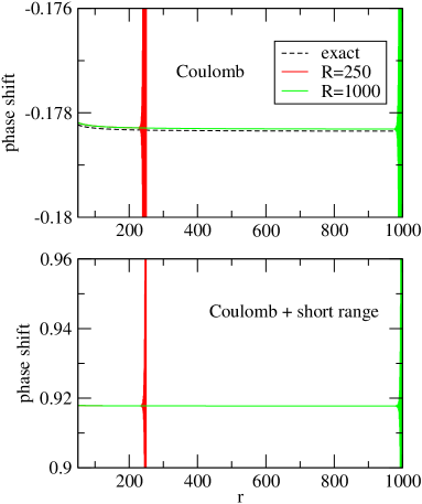
Figure 2: The local representation of the phase shift for pure Coulomb potential (upper part) and for the general case when a short range potential is added to the Coulomb term (lower part). In the first case the exact solution (dashed black line) is also displayed. For the numerical solution the boundary condition is imposed at R=250 (red line) and R=1000 (green line). Detailed discussion is given in the text.

The differential equations (53) or (54) have to be solved with the boundary conditions

$$h_{l,\theta}^{sc+}(k,0)=0$$ (56)

and

$$\lim_{r\rightarrow\infty}h_{l,\theta}^{sc+}(k,r)=0.$$ (57)

In numerical calculations instead of (57) the boundary condition

$$h_{l,\theta}^{sc+}(k,R)=0.$$ (58)

can be used. Here $R$ is a positive and otherwise arbitrary large number. The boundary condition (58) is of course an approximation and it has to be investigated how the result depends on $R$. The value of $R$ should be in the asymptotic region where (46) is satisfied.

The finite element method is chosen as a numerical technique for the solution of Eqs. (53) or (54). The method and the basis functions used in any elements are described in res00 . The same method was used also in Vol09 . For the presented calculations equally spaced finite elements of length 1 is taken. The degree of the Lobatto shape functions res00 is denoted by $N$ and the same $N$ value is used at each elements. The $\theta$ parameter of the CS was chosen to 0.1 radian.

First the pure Coulomb case is considered i.e. the potential is given by $1/r$. In this case the numerical result can be compared to the known analytical solution. The momentum was $k=3$ and the considered orbital angular momentum was $l=0$. The phase shift is calculated with the help of the local representation (51). In this equation for $\tilde{\psi}^{sc+}_{l,\theta}(k,r)$ either the exact solution or the approximate one determined by the finite element method can be used. In the second example the potential $7.5r^{2}\exp(-r)$ is added to the previous pure Coulomb term. Exactly these two cases were studied in Vol09 where a different splitting of the wave function and the exterior complex scaling method was used.

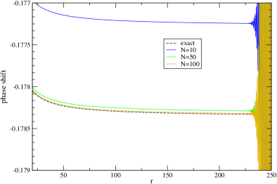
Figure 3: The local representation of the phase shift for pure Coulomb potential. In the numerical solution the boundary condition is imposed at R=250. The exact solution and the numerical ones are displayed. In the numerical calculations the number of the Lobatto shape functions $(N)$ is varied.

The upper part of Fig. 2 shows the results of the calculations carried out using pure Coulomb potential. In this case the exact solution (dashed black line) can be compared to the numerical ones. In the finite element method the boundary condition (58) is imposed at two different $R$ values ($R=250$ and $R=1000$). We note that for $r>R$ the finite element solution is not defined. The boundary condition should be set at infinity (see (57)) but a finite $R$ value is taken so it can be expected that the numerical solution is not accurate enough around the point where the boundary condition is set up. This can be clearly noticed in Fig. 2. If we choose $R=250$ then there is an oscillation with large amplitude around $r=250$. If the boundary condition is set up at a larger $R$ value then the oscillatory region is pushed out around this value. In Fig. 2 the oscillatory region moved from $r=250$ to $r=1000$ simply changing the value of the parameter $R$ from $R=250$ to $R=1000$. The effect of the boundary condition is noticeable. However, if this edge effect is not considered then the local representation of the phase shift is practically constant on a huge region. This is a useful feature since it helps to determine a unique value of phase shift of the numerical calculation. In contrast the local approximation of the phase shift in Vol09 tends to the exact value by a persistent oscillation with decreasing order of amplitude.

The lower part of Fig. 2 shows the results when the short range potential is added to the Coulomb interaction. This modification does not change the previous observations. The lower part of Fig. 2 clearly demonstrates each previous conclusions. The position of the boundary condition influences the value of the phase shift only around the point $r=R$. The phase shift calculated by the expression (51) is practically independent from the value of $r$. We note that apart from the oscillatory region around $r=250$ the two numerical solutions corresponding to the choices $R=250$ and $R=1000$ coincide in the region $50<r<250$. In this region in Fig. 2 the red and green lines are indistinguishable on the used scale.

The calculations displayed in Fig. 2 have been carried out using 50 Lobatto shape functions on each elements. We investigated the dependence of the local representation of the phase shift on the number of Lobatto functions used in the finite element method. The boundary condition (58) is set up at $R=250$. The results are depicted in Fig. 3. Apart from the region around $r=250$ the exact phase shift is reproduced with three digits accuracy with $N=50$. The calculation with $N=100$ very well reproduces the exact solution (4 digits agreement is reached almost everywhere).

It remains to check how the complex scaling parameter $\theta$ influences the calculated phase shift. Figure 4 displays the local representation of the phase shift as the function of the complex scaling parameter. Four different $r$ values are used. In these calculation the exact wave function is used in (51). If the value of $r$ is in the asymptotic region (e.g. $r=550$) then the calculated phase shift is independent from the value of the complex scaling parameter. For smaller $r$ values it is advantageous to use larger $\theta$ value to get better agreement with the exact phase shift.

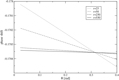
Figure 4: The local representation of the phase shift for pure Coulomb potential as the function of the complex scaling parameter. Four different $r$ values are considered and in the local representation of the phase shift the exact wave function is used.

VII Summary

We have rigorously shown that the two-body scattering problem of the pure Coulomb interaction can be solved using the standard complex scaling method. This is achieved without using any cutoff of the long range interaction. The intricate scattering boundary condition is greatly simplified and so the numerical solution can be plainly achieved. It is obvious that the suggested driven Scrödinger equation can be solved by the use of the exterior complex scaling method too. The advocated splitting of the total wave function works for general circumstances. It can be applied not only for pure Coulomb force but short range interactions can be added to the Coulomb potential. It turned out that the splitting based on the Coulomb modified plane wave does not lead to simplification of the boundary condition from the point of view of the complex scaling.

Appendix A

In the case of the splitting (32) according to (31) the source term reads

$$\tilde{S}_{l}(k,r)=\left[-\frac{1}{2r}\frac{d^{2}}{dr^{2}}r+\frac{l(l+1)}{2r^{2}}+\frac{\gamma k}{r}-\frac{k^{2}}{2}\right][\omega_{i,l}(k,r)+\chi_{l}(k,r)].$$ (59)

Since $\omega_{i,l}(k,r)$ is just the Coulomb Jost solution har ; har2 the contribution from $\omega_{i,l}(k,r)$ to the source is zero. Introducing a new variable $z=2ikr$ and rewriting the summation in (16) we have

$$\tilde{S}_{l}(k,r)=\left[-\frac{k^{2}}{2}+\frac{2k^{2}}{z}\frac{d^{2}}{dz^{2}}z-\frac{2k^{2}l(l+1)}{z^{2}}+\frac{2i\gamma k^{2}}{z}\right]\chi_{l}(z),$$ (60)

where

$$\chi_{l}(z)=\frac{e^{\gamma\pi/2}}{\Gamma(1-i\gamma)}\frac{e^{z/2}}{z}\sum_{n=0}^{l}\frac{(l+1)_{n}(-l)_{n}(1)_{n}}{(1-i\gamma)_{n}}\frac{z^{-n}}{n!}.$$ (61)

Direct calculation gives

$$\tilde{S}_{l}(k,r)=\frac{2k^{2}e^{\gamma\pi/2}}{\Gamma(1-i\gamma)}\frac{e^{z/2}}{z^{2}}\sum_{n=0}^{l}\frac{(l+1)_{n}(-l)_{n}}{(1-i\gamma)_{n}}\left(i\gamma-n+\frac{n(n+1)-l(l+1)}{z}\right)z^{-n}.$$ (62)

Rearranging the summation we get

$$\tilde{S}_{l}(k,r) = \frac{2k^{2}e^{\gamma\pi/2}}{\Gamma(1-i\gamma)}\frac{e^{z/2}}{z^{2}}\times$$ (63)

$$\qquad\times\left\{i\gamma+\sum_{n=0}^{l-1}\left[\frac{(l+1)_{n}(-l)_{n}}{(1-i\gamma)_{n}}[n(n+1)-l(l+1)]+\right.\right.$$

$$\left.\left.\qquad\qquad\qquad\qquad\qquad+(i\gamma-n-1)\frac{(l+1)_{n+1}(-l)_{n+1}}{(1-i\gamma)_{n+1}}\right]z^{-n-1}\right\}.$$

Using the fact that the Pochhammer symbols satisfy the recursion $(a)_{n+1}=(a)_{n}(a+n)$ we can show that the expression inside the square bracket is zero and so we have proved (33).

Appendix B

According to (13) in order to prove (52) it is enough to show that

$$\lim_{r\rightarrow 0}r^{l+1}\omega_{s,l}(k,r)=\lim_{r\rightarrow 0}r^{l+1}\chi_{l}(k,r).$$ (64)

From the definition (16) it follows

$$\lim_{r\rightarrow 0}r^{l+1}\chi_{l}(k,r)=e^{\gamma\pi/2}\frac{(-1)^{l}}{(2ik)^{l+1}}\frac{\Gamma(2l+1)}{\Gamma(l+1-i\gamma)}.$$ (65)

Considering (15) and the expression 7.2.2.3 prud the function $r^{l+1}\omega_{s,l}(k,r)$ is a sum of three terms

$$r^{l+1}\omega_{s,l}(k,r)=A_{l}(k,r)+B_{l}(k,r)+C_{l}(k,r),$$ (66)

where

$$A_{l}(k,r)=-K_{l}(k)\frac{M(l+1+i\gamma,2l+2;-2ikr)}{\Gamma(2l+2)\Gamma(i\gamma-l)}(-2ikr)^{2l+1}\log(-2ikr)e^{ikr},$$ (67)

$$B_{l}(k,r)=-K_{l}(k)\frac{e^{ikr}}{\Gamma(2l+2)\Gamma(i\gamma-l)}\sum_{n=0}^{\infty}f^{l}_{n}\frac{(l+1+i\gamma)_{n}}{(2l+2)_{n}}\frac{(-2ikr)^{n+2l+1}}{n!}$$ (68)

and

$$C_{l}(k,r)=-K_{l}(k)\frac{(2l)!e^{ikr}}{\Gamma(l+1+i\gamma)}\sum_{n=0}^{\infty}\frac{(i\gamma-l)_{n}}{(-2l)_{n}}\frac{(-2ikr)^{n}}{n!}.$$ (69)

The following abbreviations are used

$$K_{l}(k)=\frac{(-1)^{l+1}}{(2ik)^{l+1}}e^{2i\sigma_{l}+\gamma\pi/2}$$ (70)

and

$$f^{l}_{n}=\Psi(l+1+i\gamma+n)-\Psi(n+1)-\Psi(2l+2+n).$$ (71)

The digamma function is denoted by $\Psi(z)$. From the expressions above it is clear that $\lim_{r\rightarrow 0}A_{l}(k,r)=0$ and $\lim_{r\rightarrow 0}B_{l}(k,r)=0$. The limit value of $C_{l}(k,r)$ as $r\rightarrow 0$ is exactly the right hand side of (65) so we have proved (52).

- (1) Y.K. Ho, Phys. Rep. 99, 1 (1983).
- (2) N. Moiseyev, Phys. Rep. 302, 211 (1998).
- (3) J. Nuttall and H.L. Cohen, Phys. Rev. 188, 1542 (1969).
- (4) J.A. Hendry, Nucl. Phys. A 198, 391 (1972).
- (5) R.T. Baumel, M.C. Crocker and J. Nuttall, Phys. Rev. A 12 486 (1975).
- (6) B.R. Johnson and W.P. Reinhardt, Phys. Rev. A 29, 2933
- (7) T.N. Rescigno and C.W. McCurdy, Phys. Rev. A 31, 624 (1985)
- (8) U. Peskin and N. Moiseyev, J. Chem. Phys. 97, 6443 (1992).
- (9) T.N. Rescigno, M. Baertschy, D. Byrum and C.W. McCurdy, Phys. Rev. A 55 4253 (1997).
- (10) P.L. Bartlett, J. Phys. B: At. Mol. Opt. Phys. 39, R379 (2006).
- (11) C.W. McCurdy, D.A. Horner, T.N. Rescigno and F. Martín, Phys. Rev. A 69, 032707 (2004).
- (12) C.W. McCurdy, M. Baertschy and T.N. Rescigno, J. Phys. B: At. Mol. Opt. Phys. 37, R137 (2004).
- (13) M. Baertschy, T.N. Rescigno, W.A. Isaacs, X. Li and C.W. McCurdy, Phys. Rev. A 63, 022712 (2001).
- (14) M.V. Volkov, N. Elander, E. Yarevsky and S.L. Yakovlev, Europhys. Lett. 85, 30001(2009)
- (15) S.L. Yakovlev, M.V. Volkov, E. Yarevsky and N. Elander, J. Phys A: Math. Theor. 43, 245302 (2010).
- (16) N. Elander, M.V. Volkov,A. Larson, M. Stenrup, J.Z. Mezei, E. Yarevsky and S. Yakovlev, Few-Body Syst 45 197 (2009).
- (17) A.T. Kruppa, R. Suzuki and K. Kato, Phys. Rev. C 75, 044602 (2007).
- (18) C.W. McCurdy and F. Martin, J. Phys. B: At. Mol. Opt. Phys. 37, 917 (2004).
- (19) G. Gasaneo and L. U. Ancarani, Phys. Rev. A 82 042706 (2010).
- (20) L.U. Ancarani and G. Gasaneo, J. At. Mol. Sci. 2, 203 (2011).
- (21) J. M. Randazzo, F. Buezas, A.L. Frapiccini, F.D. Colavecchia and G. Gasaneo, Phys. Rev. A 84, 052715 (2011).
- (22) A.L. Frapiccini, J.M. Randazzo, G, Gasneo and F.D. Colavecchia, J. Phys. B: At. Mol. Opt. Phys. 43, 101001 (2010).
- (23) A.S. Kadyrov, I. Bray, A.M. Mukhamedzhanov and A.T. Stelbovics, Ann. Phys. (N.Y.) 324, 1516 (2009).
- (24) A.S. Kadyrov, I. Bray, A.M. Mukhamedzhanov and A.T. Stelbovics, Phys. Rev. A 72, 032712 (2005).
- (25) H. van Haeringen, Charged-particle interactions: theory and formulas (Coulomb Press, Leyden, 1985).
- (26) Handbook of Mathematical Functions, Eds. M. Abramowitz and I.A Stegun, Dover Publications,
- (27) H. van Haeringen, Il Nuovo Cimento 34B, 53 (1976).
- (28) A.P. Prudnikov, Yu.A. Brychkov and O.I. Marichev, Integrals and Series (Gordon and Breach Science Publishers New York, 1990).
- (29) A. Messiah, Quantum Mechanics (Dover Publications, Mineola, 1999).
- (30) Y.L. Luke, The special functions and their approximations Vol. I,(Academic Press, San Diego, 1969)
- (31) A. Erdélyi, Asymptotic Expansions (Dover Publications, New York, 1956).
- (32) T.N. Rescigno and C.W. McCurdy, Phys. Rev. A 62, 032706 (2000).