Exactly computing bivariate projection depth contours and median

Abstract. Among their competitors, projection depth and its induced estimators are very favorable because they can enjoy very high breakdown point robustness without having to pay the price of low efficiency, meanwhile providing a promising center-outward ordering of multi-dimensional data. However, their further applications have been severely hindered due to their computational challenge in practice. In this paper, we derive a simple form of the projection depth function, when $(\mu,\sigma)$ = (Med, MAD). This simple form enables us to extend the existing result of point-wise exact computation of projection depth (PD) of Zuo and Lai (2011) to depth contours and median for bivariate data.

Key words: Projection depth; Projection median; Projection depth contour; Exact computation algorithm; Linear fractional functionals programming;

2000 Mathematics Subject Classification Codes: 62F10; 62F40; 62F35

1 Introduction

To generalize order-related univariate statistical methods, depth functions have emerged as powerful tools for nonparametric multivariate analysis with the ability to provide a center-outward ordering of the multivariate observations. Points deep inside a data cloud get higher depth and those on the outskirts receive lower depth. Such depth induced ordering enables one to develop favorable new robust estimators of multivariate location and scatter matrix. Since Tukey’s introduction (Tukey, 1975), depth functions have gained much attention in the last two decades. Numerous depth notations have been introduced. To name a few, halfspace depth (Tukey, 1975), simplicial depth (Liu, 1990), regression depth (Rousseeuw and Hubert, 1999), projection depth (Liu, 1992; Zuo and Serfling, 2000; Zuo, 2003).

Zuo and Serfling (2000) and Zuo (2003) found that among all the examined depth notions, projection depth is one of the favorite, enjoying very desirable properties. Furthermore, projection depth induced robust estimators, such as projection depth weighted means and median, can possess a very high breakdown point as well as high relative efficiency with appropriate choices of univariate location and scale estimators, serving as very favorable alternatives to the regular mean (Zuo, 2003; Zuo et al., 2004). In fact, projection depth weighted means include as a special case the famous Donoho-Stahel estimator (Stahel, 1981; Donoho, 1982; Tyler, 1994; Maronna et al., 1995; Zuo et al., 2004), the latter is the first constructed location estimator in high dimensions enjoying high breakdown point robustness and affine equivariance, while the projection depth median has the highest breakdown point among all the existing affine equivariant multivariate location estimators (Zuo, 2003).

However, the further prevalence of projection depth and its induced estimators is severely hindered by their computational intensity and intimidation. The computation of projection depth seems intractable since it involves supremum over infinitely many direction vectors. There were only approximating algorithms in the last three decades until Zuo and Lai (2011), in which they proved that there is no need to calculate the supremum over infinitely many direction vectors in the bivariate data when the outlyingness function uses the very popular choice (Med, MAD) as the univariate location and scale pair. An exact algorithm for projection depth and its weighted mean, i.e. Donoho-Stahel estimator, was also constructed in that paper.

In the current paper, we further generalize their idea to the higher dimensional cases by utilizing linear fractional functionals programming (Swarup, 1962). That is, we find that, with the choice of (Med, MAD), we only need to calculate the supremum over a finite number of direction vectors for $p\geq 2$. Furthermore, these direction vectors are $x$-free and depend only on the data cloud. Therefore, we derive a simple form of the projection depth function, and are able to compute the bivariate projection depth contours and median very conveniently through linear programming based on the procedure of Zuo and Lai (2011). It is found that sample projection depth contours are polyhedral under some mild conditions. Furthermore, it is noteworthy that the computational methods discussed in this paper have no limitation on the dimension $p$, and therefore could possible be implemented to spaces with $p>2$, as well as to the modified projection depth (Šiman, 2011) in a more general multidimensional regression context. The corresponding programs are available from the authors (zuo@msu.edu or csuliuxh912@gmail.com).

The rest of the paper is organized as follows. Section 2 provides the definitions of the projection depth contour and projection median. Section 3 presents the main idea of how to get a simple form of the projection depth function. Section 4 discusses the exact computational issue of the projection depth contour and projection median by linear programming. While some numerical examples are given in Section 5.

2 Definition

For a given distribution $F$ on $\mathbb{R}^{1}$, let $\mu(F)$ be translation equivariant and scale invariant, and $\sigma(F)$ be translation invariant and scale equivariant. Define the outlyingness of a point $x\in R^{p}\ (p\geq 1)$ with respect to the distribution $F$ of the random variable $X\in R^{p}$ as (see (Zuo, 2003) and references therein)

$$O(x,F)=\sup_{\|u\|=1}|Q(u,x,F)|$$ (1)

where $Q(u,x,F)=(u^{\tau}x-\mu(F_{u}))/\sigma(F_{u})$, if $u^{\tau}x-\mu(F_{u})=\sigma(F_{u})=0$, then define $Q(u,x,F)=0$. $F_{u}$ is the distribution of $u^{\tau}X$, which is the projection of $X$ onto the unit vector $u$.

Throughout this paper, we select the very popular robust choice of $\mu$ and $\sigma$: the median (Med) and the median absolute deviation (MAD). Based on definition (1), the projection depth of any given point $x$ with respective to $F$, ${\mbox{\it PD}}(x,F)$, can then be defined as (Liu, 1992; Zuo and Serfling, 2000; Zuo, 2003)

$${\mbox{\it PD}}(x,F)=1/(1+O(x,F))$$

With the outlyingness function and projection depth function defined above, we then define the projection depth median (PM) and contours (PC) as follows (Zuo, 2003)

$$PM(F)=\mbox{arg}\max\limits_{x\in R^{p}}PD(x,F),$$

$$PC(\alpha,F)=\left\{x\in R^{p}:PD(x,F)=\alpha\right\},$$

where $0<\alpha\leq\alpha^{*}=\sup_{x\in R^{p}}PD(x,F)$.

For a given sample $\mathcal{X}^{n}=\{X_{1},X_{2},\cdots,X_{n}\}$ from $X$, let $F_{n}$ be the corresponding empirical distribution. By simply replacing $F$ by $F_{n}$ in $PM(F)$ and $PC(\alpha,F)$, we can obtain their sample version: $PM(F_{n})$ and $PC(\alpha,F_{n})$. Without confusion, we use $\mathcal{X}^{n}$ and $F_{n}$ interchangeably in what follows. Furthermore, by noting the fact that for the choice of (Med, MAD), $Q(u,x,\mathcal{X}^{n})$ in (1) is odd with respect to $u$, we drop the absolute value sign existing in definition (1), and consider

$$O(x,\mathcal{X}^{n})=\sup\limits_{\|u\|=1}Q(u,x,\mathcal{X}^{n})$$

instead in what follows, where

$$Q(u,x,\mathcal{X}^{n})=\frac{u^{\tau}x-\mbox{Med}(u^{\tau}\mathcal{X}^{n})}{\mbox{MAD}(u^{\tau}\mathcal{X}^{n})},$$

where $u^{\tau}x$ denotes the projection of $x$ onto the unit vector $u$, and $u^{\tau}\mathcal{X}^{n}=\left\{u^{\tau}X_{1},u^{\tau}X_{2},\cdots,u^{\tau}X_{n}\right\}$. Let $Z_{(1)}\leq Z_{(2)}\leq,\cdots,\leq Z_{(n)}$ be the order statistics based on the univariate random variables $\mathcal{Z}^{n}=\{Z_{1},Z_{2},\cdots,Z_{n}\}$, then

$$\mbox{Med}(\mathcal{Z}^{n})=\frac{Z_{(\lfloor(n+1)/2\rfloor)}+Z_{(\lfloor(n+2)/2\rfloor)}}{2},$$

$$\mbox{MAD}(\mathcal{Z}^{n})=\mbox{Med}\{|Z_{i}-\mbox{Med}(Z^{n})|,i=1,2,\cdots,n\},$$

where $\lfloor\cdot\rfloor$ is the floor function.

3 The main idea

Note that, for any given sample $\mathcal{X}^{n}$, the tasks of computing both $PM(\mathcal{X}^{n})$ and $PC(\alpha,\mathcal{X}^{n})$ mainly involve $O(x,\mathcal{X}^{n})$, i.e.

$$PM(\mathcal{X}^{n})=\mbox{arg}\min\limits_{x\in R^{p}}O(x,\mathcal{X}^{n}),$$

$$PC(\alpha,\mathcal{X}^{n})=\left\{x\in R^{p}:O(x,\mathcal{X}^{n})=\beta\right\},$$

where $\beta=1/\alpha-1$. Thus, let’s first focus on the computation of $O(x,\mathcal{X}^{n})$. Without loss of generality, in what follows, we assume $\mathcal{X}^{n}$ to be in general position, which is commonly used in most existing literature; see for example Donoho and Gasko (1992).

By the idea of a circular sequence (Edelsbrunner, 1987) (see also Dyckerhoff (2000); Cascos (2007)), for any given unit vector $v\in\mathcal{S}=\{u\in R^{p}:\|u\|=1\}$, there must exist two permutations, say $(i_{1},i_{2},\cdots,i_{n})$ and $(j_{1},j_{2},\cdots,j_{n})$, of $(1,2,\cdots,n)$ such that

$$v^{\tau}X_{i_{1}}\leq v^{\tau}X_{i_{2}}\leq\cdots\leq v^{\tau}X_{i_{n}},$$

$$Y_{j_{1}}\leq Y_{j_{2}}\leq\cdots\leq Y_{j_{n}},$$

where $Y_{j_{l}}=|v^{\tau}X_{j_{l}}-\mbox{Med}(v^{\tau}\mathcal{X}^{n})|,\ (1\leq l\leq n)$. There is a small non-empty set $\mathcal{N}(v)\subset\mathcal{S}$ of $v$ such that these hold true for any $v\in\mathcal{N}(v)$. This implies that the whole unit sphere $\mathcal{S}$ can be covered completely by at most $N$ (with order $O\big{(}{n\choose p}^{2}\big{)}$) non-empty fragments $S_{k}=\{v\in\mathcal{S}$: $v$ satisfy constraint conditions $\mathcal{Q}_{k}\}$ with $\mathcal{Q}_{k}$ being

$$\left\{\begin{array}[]{c}v^{\tau}(X_{i_{k,2}}-X_{i_{k,1}})\geq 0,\\ v^{\tau}(X_{i_{k,3}}-X_{i_{k,2}})\geq 0,\\ \vdots\\ v^{\tau}(X_{i_{k,n}}-X_{i_{k,n-1}})\geq 0,\\ Y_{j_{k,2}}-Y_{j_{k,1}}\geq 0,\\ Y_{j_{k,3}}-Y_{j_{k,2}}\geq 0,\\ \vdots\\ Y_{j_{k,n}}-Y_{j_{k,n-1}}\geq 0,\\ \|v\|=1,\end{array}\right.$$

for some fixed permutations $(i_{k,1},i_{k,2},\cdots,i_{k,n})$ and $(j_{k,1},j_{k,2},\cdots,j_{k,n})$ of $(1,\cdots,n)$, where $1\leq k\leq N$.

Note that different fragments $S_{k}\ (k=1,2,\cdots,N)$ are connected and overlapped with each other only on the boundaries. Thus, to calculate $O(x,\mathcal{X}^{n})$, it is sufficient to calculate

$$O(x,\mathcal{X}^{n})=\max_{1\leq k\leq N}O_{k}(x,\mathcal{X}^{n})$$

with

$$O_{k}(x,\mathcal{X}^{n})=\sup\limits_{u\in S_{k}}Q(u,x,\mathcal{X}^{n}).$$ (2)

Furthermore, from the definition and property of $S_{k}$, it is easy to see that, for any $u\in S_{k}$, the outlyingness function $Q(u,x,\mathcal{X}^{n})$ can be simplified to

$$Q(u,x,\mathcal{X}^{n})=\frac{u^{\tau}(x-X_{i_{k,m}})}{|u^{\tau}X_{j_{k,m}}-u^{\tau}X_{i_{k,m}}|},$$ (3)

if $n$ is odd with $m=(n+1)/2$, otherwise

$$Q(u,x,\mathcal{X}^{n})=\frac{2u^{\tau}\left(x-X_{k,a}\right)}{\left|u^{\tau}\left(X_{j_{k,m}}-X_{k,a}\right)\right|+\left|u^{\tau}\left(X_{j_{k,m^{*}}}-X_{k,a}\right)\right|},$$ (4)

with $m=n/2$, $m^{*}=m+1$ and $X_{k,a}=(X_{i_{k,m}}+X_{i_{k,m^{*}}})/2$.

Remark 1. Based on the assumption that $\mathcal{X}^{n}$ are in general position, the denominators in the above two formulas will not be 0 for all $u\in S_{k}$, since they are actually equal to MAD($u^{\tau}\mathcal{X}^{n}$), and greater than 0 under such an assumption when $n\geq 2p$; see the proof of Theorem 3.4 in Zuo (2003).

By (3) and (4), we obtain the following proposition.

Proposition 1. Assume $\mathcal{X}^{n}$ is in general position. Then for any given $k$ $(1\leq k\leq N)$, the optimization problem (2) is equivalent to

$$O_{k}(x,\mathcal{X}^{n})=\sup_{z}\frac{c_{k}^{\tau}z}{d_{k}^{\tau}z},$$ (5)

subject to

$$A_{k}z\geq 0$$ (6)

where $c_{k},d_{k}$ and $A_{k}$ will be specified in the Appendix. Here $\textbf{b}\geq 0$ means that b is component-wise non-negative if b is a vector, i.e. for any component $\textbf{b}_{i}$, we have $\textbf{b}_{i}\geq 0$.

(5) with constraint conditions (6) is typically a linear fractional functionals programming problem. By theorem 1 of Swarup (1962) (see also Šiman (2011) (p. 950) for more general discussion), it is easy to show that the maximum of $c_{k}^{\tau}z/d_{k}^{\tau}z$ will only occur at the basic feasible solution of (6). Note that the number of fragments $S_{k}$ is limited (at most $N$). Thus, we have

Theorem 1. Suppose that the choice of location and scale measures of projection depth function is the pair (Med, MAD). Then the number of direction vectors needed to compute the projection depth exactly is finite. Furthermore, these direction vectors only depend on the data cloud $\mathcal{X}^{n}$.

Remark 2. The idea of dividing the unit sphere $\mathcal{S}$ into fragments $S_{k}$ by applying Med and MAD sequences was first used in Zuo and Lai (2011) for computing the bivariate projection depth; see also Paindavein and Šiman (2011b, c) for other similar applications. Here we extend the result of Zuo and Lai (2011) to $R^{p}$ ($p\geq 2$). That is, one could compute PD in $R^{p}$ exactly by only considering a finite number of direction vectors. Furthermore, the $x$-free property of these direction vectors can bring convenience to the computation of PD$(x,\mathcal{X}^{n})$ for any $x$, since we only need to search the direction vectors once.

4 Exact computation of $PM(\mathcal{X}^{n})$ and $PC(\alpha,\mathcal{X}^{n})$

From the discussion above, we can obtain the two following observations, namely, for any given $x$,

• the way to divide sphere $\mathcal{S}$ into fragments $S_{k}\ (k=1,2,\cdots,N)$ is fixed, i.e. $x$-free, as long as the data cloud $\mathcal{X}^{n}$ is fixed.

• there is no need to calculate $Q(u,x,\mathcal{X}^{n})$ over an infinite number of direction vectors. It is enough to calculate it for, say, $u_{1},u_{2},\cdots,u_{M}$.

Based on the discussion and two observations above, we therefore can re-express the outlyingness function $O(x,\mathcal{X}^{n})$ as follows

$$O(x,\mathcal{X}^{n})=\max\left\{\frac{u_{1}^{\tau}x-\text{Med}(u_{1}^{\tau}\mathcal{X}^{n})}{\text{MAD}(u_{1}^{\tau}\mathcal{X}^{n})},\frac{u_{2}^{\tau}x-\text{Med}(u_{2}^{\tau}\mathcal{X}^{n})}{\text{MAD}(u_{2}^{\tau}\mathcal{X}^{n})},\cdots,\frac{u_{M}^{\tau}x-\text{Med}(u_{M}^{\tau}\mathcal{X}^{n})}{\text{MAD}(u_{M}^{\tau}\mathcal{X}^{n})}\right\},$$

where $\{u_{i}\}_{i=1}^{M}$ are some $p$-dimensional vectors depending only on the data cloud $\mathcal{X}^{n}$. For the sake of convenience, hereafter we write $g_{i}(x)=\textbf{a}_{i}^{\tau}x-b_{i}$ $(i=1,2,\cdots,M)$, where $\textbf{a}_{i}=\frac{1}{\text{MAD}(u_{i}^{\tau}\mathcal{X}^{n})}u_{i}$ and $b_{i}=\frac{\text{Med}(u_{i}^{\tau}\mathcal{X}^{n})}{\text{MAD}(u_{i}^{\tau}\mathcal{X}^{n})}$.

Obviously, $O(x,\mathcal{X}^{n})=\max_{1\leq i\leq M}\{g_{i}(x)\}$ is in fact a piece-wise linear convex function with respect to $x$ for the given data cloud $\mathcal{X}^{n}$. Therefore, its minimizers can be found by using common linear programming methods by solving the problem

$$s=\min_{z}\ t$$

subject to

$$t\geq g_{i}(x),\ i=1,2,\cdots,M,$$

where $z=(t,x^{\tau})^{\tau}$. This kind of problem can be solved by some common solver such as linprog.m in Matlab. Let $z_{0}=(t_{0},x_{0}^{\tau})^{\tau}$ be a final solution of this problem. Then, it is easy to show that $x_{0}$ is one of the deepest points with depth value $PD(x_{0},\mathcal{X}^{n})=1/(1+t_{0})=\alpha^{*}$.

Given the nature of the maximum piece-wise linear convex function $\max_{1\leq i\leq M}g_{i}(x)$, there is either a single minimizer or a convex polyhedral set of minimizers. Then there naturally comes a question, namely, after obtaining the value $\alpha^{*}$, how to get all of these vertexes? Note that the projection median is a specific case of the projection depth contour. Therefore, let’s focus now on the computation of projection depth contours. For any given $0<\alpha\leq\alpha^{*}$, the projection depth contour is the boundary of the projection depth region (Zuo, 2003),

$$PR(\alpha,\mathcal{X}^{n}) = \left\{x\in R^{p}:PD(x,\mathcal{X}^{n})\geq\alpha\right\}$$

$$= \left\{x\in R^{p}:O(x,\mathcal{X}^{n})\leq\beta\right\}$$

$$= \left\{x\in R^{p}:g_{i}(x)\leq\beta,i=1,2,\cdots,M\right\}.$$

Typically, the regions constrained by linear inequalities such as

$$g_{i}(x)\leq\beta,i=1,2,\cdots,M$$ (7)

are polytopes. Therefore, the boundary of $PR(\alpha,\mathcal{X}^{n})$, i.e. $PC(\alpha,\mathcal{X}^{n})$, could be easily found by employing procedures such as qhull (Barber et al., 1996) based on the dual relationship between vertex and facet enumeration (Bremner et al., 1998); see also Paindavein and Šiman (2011a). In Matlab, these kinds of tasks can be fulfilled by the function con2vert.m, which was developed by Michael Kleder, and can be downloaded from Matlab Central File Exchange.

However, in many practical applications, the number $M$ (with order $O\big{(}{n\choose p}^{2}\big{)}$) of the direction vectors may be very large. When $M$ is too large, it is difficult to obtain the boundary of the region formed by (7) by using some of the aforementioned procedures such as con2vert.m, since they involve solving some large generalized inverse matrices. Therefore, it is important to eliminate some redundant constraints before computing $PC(\alpha,\mathcal{X}^{n})$ for too large $M$.

Note that, for any given $\alpha$ $(0<\alpha\leq\alpha^{*})$, the number of the non-redundant constraints in (7) is much small compared to $M$, which implies that numerous inequalities in (7) could be eliminated during the computation of the $\alpha$-contour. In fact, it is not difficult to show that

$$PR(\alpha,\mathcal{X}^{n})=\mathcal{C}_{1}\cap\mathcal{C}_{2}\cap\cdots\cap\mathcal{C}_{s},$$

where $\mathcal{C}_{k}=\{x:g_{j}(x)\leq\beta,j=i_{k},i_{k}+1,\cdots,i_{k+1}\}$ with $1\leq k\leq s-1$ and $1=i_{1}<i_{2}<\cdots<i_{s}=M$, and that $\mathcal{C}_{k}$ is non-empty if $\min_{1\leq l\leq s-1}\{i_{l+1}-i_{l}\}\gg p$. Then, when $M$ is large, a procedure for exactly computing $PC(\alpha,\mathcal{X}^{n})$ is: (1), to find the non-redundant constraints in each $\mathcal{C}_{i}$ at first, then (2), to use all of these non-redundant constrains together to compute $PC(\alpha,\mathcal{X}^{n})$.

With the vertexes in hand, some common graphical packages could be employed to visualize these contours very easily in spaces of $p=2,3$. It is noteworthy that, although all the methods discussed above could possible be implemented to spaces with $p\geq 2$ theoretically, feasible exact algorithm for computing the projection depth exists now only in the bivariate data (Zuo and Lai, 2011). Therefore, we can only provide some exactly results about the bivariate projection depth contours and projection median in the current paper. All the direction vectors $\{u_{1},\cdots,u_{M}\}$ are found by using the procedure of Zuo and Lai (2011). The $x$-free property of these vectors can be proved similarly by using the linear fractional functionals programming as Proposition 1.

5 Numerical analysis

In order to gain more insight into the sample version of projection depth contours and projection median, we construct some numerical examples in this section.

5.1 Simulation results

To illustrate the robustness and the shape of the bivariate projection depth contours and median, we present two examples as follows. The data are mainly generated from the normal distribution, but contain a few outliers.

Example 1. We first generate 60 samples $X=(X_{1},X_{2})^{\tau}$ from the normal distribution $N(0,I_{2})$, and then disturb these samples randomly by replacing their first components by 6 with probability 0.05.

Example 2. We first generate 400 samples $X=(X_{1},X_{2})^{\tau}$ from the normal distribution $N(0,\Sigma_{0})$, and then disturb these samples randomly by replacing their first components by 6 with probability 0.10, where

$$\Sigma_{0}=\left(\begin{array}[]{lr}1&0.5\\ 0.5&1\end{array}\right).$$

For the sake of comparison, the population versions of $PC(\alpha,X)$ corresponding to these two examples are also provided here, and plotted according to the formula

$$(x_{1},x_{2})\times\Sigma^{-1}\times{x_{1}\choose x_{2}}=\frac{C_{N}^{2}(1-\alpha)^{2}}{\alpha^{2}},$$

which was developed in Zuo (2003). Here $C_{N}=\Phi^{-1}(\frac{3}{4})\approx 0.6744898$, $\Sigma$ denotes the covariance matrix of normally distribution $X$, namely, $I_{2}$ in example 1 and $\Sigma_{0}$ in example 2. The population versions $PC(\alpha,X)$ of example 1 and 2 are given in Figure 2 and 4, respectively, while the sample versions $PC(\alpha,\mathcal{X}^{n})$ are plotted in Figure 2 and 4, respectively.

Comparing the figures of sample versions with those of population, it is ready to see that

• The sample versions $PC(\alpha,\mathcal{X}^{n})$ are roughly elliptical, similar to the shapes of the population versions $PC(\alpha,X)$. Furthermore, it is remarkable that they are resistant to the notorious vertical outliers in Figure 2 and 4. These results confirm that $PC(\alpha,\mathcal{X}^{n})$ are very robust, and could capture the feature of $PC(\alpha,X)$ (Zuo, 2003), even when there are a few outliers.

• It is very interesting to note that the shapes of the projection depth contours are also polylateral due to the properties of the function $\max_{1\leq i\leq M}g_{i}(x)$, similar to that of halfspace depth contours (Ruts and Rousseeuw, 1996). On the other hand, unlike halfspace depth contours, $PC(\alpha,\mathcal{X}^{n})$ does not need to pass through the observations.

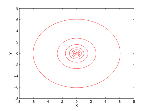
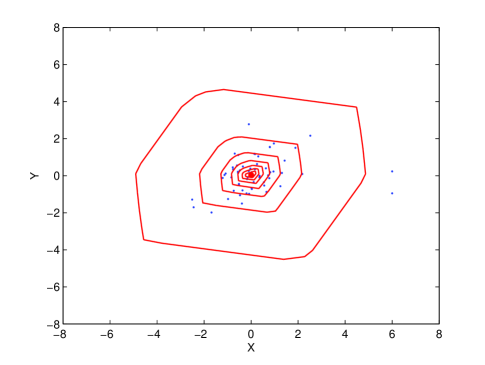
Figure 1: Population version $PC(\alpha,X)$ for Example 1 with $\alpha=0.1,0.2,\cdots,0.9$ (from out to center).

Figure 2: Sample version $PC(\alpha,\mathcal{X}^{n})$ for $\alpha=0.1,0.2,\cdots,0.7$ (from out to center). Here the most inner big point denotes the projection median.

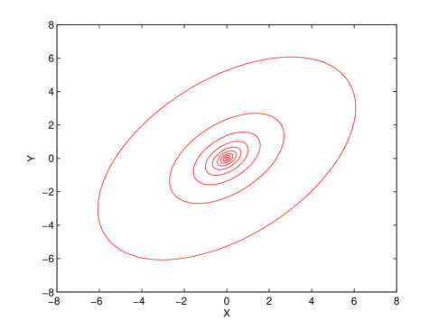
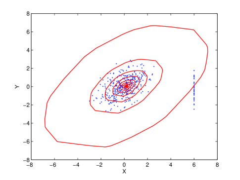
Figure 3: Population version $PC(\alpha,X)$ for Example 2 with $\alpha=0.1,0.2,\cdots,0.9$ (from out to center)

Figure 4: Sample version $PC(\alpha,\mathcal{X}^{n})$ for $\alpha=0.1,0.2,\cdots,0.8$ (from out to center). Similar to Figure 2, the most inner big point is also the computed projection median.

Furthermore, to gain more information about the shape of the projection depth contours, we also provide some other examples in the following. The sample size we used is 2500. Here Figure 6 reports the projection depth contours $PC(\alpha,\mathcal{X}^{n})$ corresponding to the uniform distribution over the triangle with its vertexes being $(0,0)$, $(0,1)$ and $(1,1)$. Figure 6 corresponds to the uniform distribution over region $[0,1]\times[0,1]$. Figure 8 gives the contours of the normal distribution $N(0,I_{2})$. While Figure 8 provides the contours of $\delta X+(1-\delta)Y$, where $X\sim N(\mu_{1},I_{2})$, $Y\sim N(\mu_{2},I_{2})$, $\mu_{1}=(-2,-2)$, $\mu_{2}=(2,2)$, and $\delta$ is a discrete random variable with probability 0.5 taking value 1 and 0.5 taking value 0. Here $X$, $Y$ and $\delta$ are all independently disturbed. From these figures, we can see that the projection contours are also polylateral and convex.

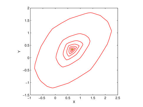
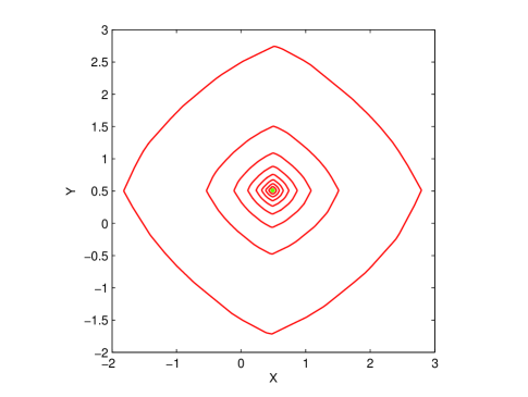
Figure 5: Projection depth contours of the uniform distribution over the triangle formed by vertexes: $(0,0)$, $(0,1)$ and $(1,1)$, where $\alpha=0.1,0.2,\cdots,0.7$ (from out to center).

Figure 6: Projection depth contours of the uniform distribution over $[0,1]\times[0,1]$, where $\alpha=0.1,0.2,\cdots,0.9$ (from out to center).

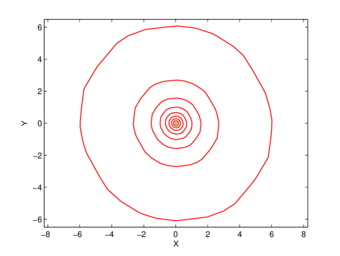
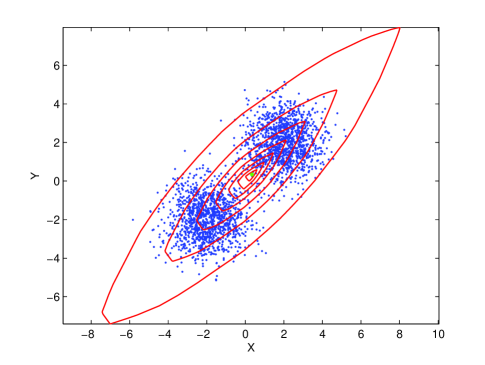
Figure 7: Projection depth contours of the bivariate standard normal distribution $N(0,I_{2})$, where $\alpha=0.1,0.2,\cdots,0.9$ (from out to center).

Figure 8: Projection depth contours of the random vector $\delta X+(1-\delta)Y$, where $\alpha=0.2,0.3,\cdots,0.9$ (from out to center).

5.2 Real data example

Here a real data example is presented to illustrate the performance of projection depth contours.

Table 1 here is taken from Table 7 of Rousseeuw and Leroy (1987) (p.57). Total 28 animals’ brain weight (in grams) and body weight (in kilograms) are presented in this table. Before the analysis, logarithmic transformation was taken for the sake of convenience. According to the results of Rousseeuw and Leroy (1987), there are five cases considered as outlying, i.e. diplodocus, human, triceratops, rhesus monkey and brachiosaurus. Among them, the most severe cases are diplodocus, triceratops and brachiosaurus. In fact, these three cases are referred to as dinosaurs because they possess a small brain as compared with a heavy body (see Table 1) and their highly negative residuals can lead to a low slope for the least squares fit. For the remaining two cases, although their actual brain weights are higher than those predicted by the linear model, they are not worse than the three previous cases since they do not obey the same trend as that one followed by the majority of the data.

Table 1: Body and Brain Weight for 28 Animals (Rousseeuw and Leroy, 1987).

	Index		Body Weight	Brain Weight
	$i$	Species	$X_{i}$	$Y_{i}$
	1	Mountain beaver	1.350	8.100
	2	Cow	465.000	423.000
	3	Gray wolf	36.330	119.500
	4	Goat	27.660	115.000
	5	Guinea pig	1.040	5.500
	6	Diplodocus	11700.000	50.000
	7	Asian elephant	2547.000	4603.000
	8	Donkey	187.100	419.000
	9	Horse	521.000	655.000
	10	Potar monkey	10.000	115.000
	11	Cat	3.300	25.600
	12	Giraffe	529.000	680.000
	13	Gorilla	207.000	406.000
	14	Human	62.000	1320.000
	15	African elephant	6654.000	5712.000
	16	Triceratops	9400.000	70.000
	17	Rhesus monkey	6.800	179.000
	18	Kangaroo	35.000	56.000
	19	Hamster	0.120	1.000
	20	Mouse	0.023	0.400
	21	Rabbit	2.500	12.100
	22	Sheep	55.500	175.000
	23	Jaguar	100.000	157.000
	24	Chimpanzee	52.160	440.000
	25	Brachiosaurus	87000.000	154.500
	26	Rat	0.280	1.900
	27	Mole	0.122	3.000
	28	Pig	192.000	180.000

We plot the projection depth contours in Figure 10, where the green point is the projection median with depth value 0.73257, five labeled points denote the outliers mentioned above with the points 1-3 corresponding to the case of diplodocus, triceratops and brachiosaurus and 4-5 corresponding to those of human and rhesus monkey. 8 contours are plotted there. From Figure 10, we can see that all of these three dinosaurs lie outside the contour 0.1, while points 4-5 lie between the contours 0.1 and 0.15. These results are consistent with those of Rousseeuw and Leroy (1987), implying that projection depth contours can capture the structures of the objective data and identify outliers.

Furthermore, it is worth mentioning that the shape of these plotted contours is not affected by a few atypical points at the outskirts of the cloud, namely, both the inner and outer depth contours are roughly elliptical, unlike those of halfspace depth contours (see Figure 10) (Ruts and Rousseeuw, 1996). This is the most outstanding difference between projection and halfspace depth contours, confirming the more robustness property of projection depth and its contours (see Zuo (2004)).

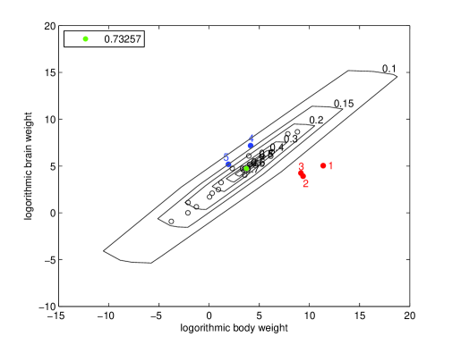
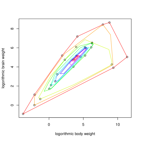
Figure 9: Projection depth contours with $\alpha=0.7,0.6,\cdots,0.2,0.15,0.1$ (from center to out).

Figure 10: Halfspace depth contours (Ruts and Rousseeuw, 1996).

Appendix Proofs of main results

Proof of Proposition 1. Here, without loss of generality, we prove only the odd $n$ case. Note that, for any $u\in\mathcal{Q}_{k}$, we have

$$u^{T}X_{i_{1}}\leq u^{T}X_{i_{2}}\leq\cdots\leq u^{T}X_{i_{m}}\leq\cdots\leq u^{T}X_{i_{n}}$$

according to the definition of $\mathcal{Q}_{k}$. This implies that

$$|u^{T}(X_{i}-X_{i_{k,m}})|=\left\{\begin{array}[]{ll}-u^{T}(X_{i}-X_{i_{k,m}}),&\quad\text{if }i\in\{i_{k,1},i_{k,2},\cdots,i_{k,m-1}\},\\ u^{T}(X_{i}-X_{i_{k,m}}),&\quad\text{if }i\in\{i_{k,m},i_{k,m+1},\cdots,i_{k,n}\}.\end{array}\right.$$

That is, we can remove the absolute value signs of $Y_{j_{l}}$ based on the order information existing in the permutation $(i_{k,1},i_{k,2},\cdots,i_{k,n})$. Therefore, for any $u\in\mathcal{Q}_{k}$, (3) can be further simplified to

$$Q(u,x,\mathcal{X}^{n})=\frac{c_{k}^{T}u}{d_{k}^{T}u}$$

where $c_{k}=x-X_{i_{k},m}$ and $d_{k}=s_{k}(j_{k,m})\cdot(X_{j_{k},m}-X_{i_{k},m})$ $(1\leq k\leq N)$, with

$$s_{k}(i)=\left\{\begin{array}[]{ll}-1,&\quad\text{if }i\in\{i_{k,1},i_{k,2},\cdots,i_{k,m-1}\},\\ 1,&\quad\text{if }i\in\{i_{k,m},i_{k,m+1},\cdots,i_{k,n}\}.\end{array}\right.$$

Next, note that, for any positive $\lambda$ and $z=\lambda u$, it holds that $c_{k}^{\tau}z/d_{k}^{\tau}z=c_{k}^{\tau}u/d_{k}^{\tau}u$ and $b_{k}^{\tau}z\geq 0$ if $b_{k}^{\tau}u\geq 0$. Then, (3) and constrain condition $\mathcal{Q}_{k}$ lead to

$$O_{k}(x,\mathcal{X}^{n})=\sup_{z}\frac{c_{k}^{\tau}z}{d_{k}^{\tau}w}$$ (8)

subject to

$$A_{k}z\geq 0$$

$1\leq k\leq N$, with $A_{k}={A_{k1}\choose A_{k2}}$, where

$$A_{k1}=(X_{i_{k,2}}^{\tau}-X_{i_{k,1}}^{\tau},X_{i_{k,3}}^{\tau}-X_{i_{k,2}}^{\tau},\cdots,X_{i_{k,n}}^{\tau}-X_{i_{k,n-1}}^{\tau})^{\tau}$$

and

$$A_{k2}=\left(\begin{array}[]{c}s_{k}(j_{k,2})\cdot(X_{j_{k,2}}^{\tau}-X_{i_{k,m}}^{\tau})-s_{k}(j_{k,1})\cdot(X_{j_{k,1}}^{\tau}-X_{i_{k,m}}^{\tau})\\ s_{k}(j_{k,3})\cdot(X_{j_{k,3}}^{\tau}-X_{i_{k,m}}^{\tau})-s_{k}(j_{k,2})\cdot(X_{j_{k,2}}^{\tau}-X_{i_{k,m}}^{\tau})\\ \vdots\\ s_{k}(j_{k,n})\cdot(X_{j_{k,n}}^{\tau}-X_{i_{k,m}}^{\tau})-s_{k}(j_{k,n-1})\cdot(X_{j_{k,n-1}}^{\tau}-X_{i_{k,m}}^{\tau})\end{array}\right).$$

This completes the proof of Proposition 1.

References

- Barber et al. (1996) Barber, C.B., Dobkin, D.P., Huhdanpaa, H., (1996). The quickhull algorithm for convex hulls. ACM Transactions on Mathematical Software 22: 469-483.
- Bremner et al. (1998) Bremner, D., Fukuda, K., Marzetta, A., (1998). Primal-dual methods for vertex and facet enumeration. Discrete and Computational Geometry, 20: 333-357.
- Cascos (2007) Cascos, I. (2007). The expected convex hull trimmed regions of a sample. Computational Statistics, 22, 557-569.
- Donoho (1982) Donoho, D.L., 1982. Breakdown properties of multivariate location estimators. Ph.D. Qualifying Paper. Dept. Statistics, Harvard University.
- Donoho and Gasko (1992) Donoho, D.L. and Gasko, M. (1992). Breakdown properties of location estimates based on halfspace depth and projected outlyingness. Ann. Statist., 20: 1808-1827.
- Dyckerhoff (2000) Dyckerhoff, R. (2000). Computing zonoid trimmed regions of bivariate data sets. In J. Bethlehem and P. van der Heijden, eds., COMPSTAT 2000. Proceedings in Computational Statistics, 295-300. Physica, Heidelberg.
- Edelsbrunner (1987) Edelsbrunner, H. (1987). Algorithms in Combinatorial Geometry. Springer, Heidelberg.
- Halin et al. (2010) Halin, M., Paindaveine, D. and Šiman, M. (2010). Multivariate quantiles and multiple-output regression quantiles: From L1 optimization to halfspace depth. Ann. Statist., 38(2): 635-669.
- Liu (1990) Liu, R. Y. (1990). On a notion of data depth based on random simplices. Ann. Statist., 18: 191-219.
- Liu (1992) Liu, R. Y. (1992). Data depth and multivariate rank tests. In L1-Statistical Analysis and Related Methods (Y. Dodge, ed.) 279-294. North-Holland, Amsterdam.
- Maronna et al. (1995) Maronna, R.A., Yohai, V.J., 1995. The behavior of the Stahel-Donoho robust multivariate estimator. J. Amer. Statist. Assoc. 90, 330-341.
- Paindavein and Šiman (2011a) Paindaveine, D., Šiman, M. (2011a). Computing multiple-output regression quantile regions. Comput. Statist. Data Anal., In press.
- Paindavein and Šiman (2011b) Paindaveine, D., Šiman, M. (2011b). On directional multiple-output quantile regression. J. Multivariate Anal., 102, 193-392.
- Paindavein and Šiman (2011c) Paindaveine, D., Šiman, M. (2011c). Computing multiple-output regression quantile regions from projection quantiles. Comput. Statist., In press.
- Rousseeuw and Leroy (1987) Rousseeuw, P.J. and A. Leroy. (1987). Robust regression and outlier detection. Wiley New York, 1987.
- Rousseeuw and Hubert (1999) Rousseeuw, P.J. and Hubert, M. (1999). Regression depth (with discussion). J. Amer. Statist. Assoc., 94: 388-433.
- Ruts and Rousseeuw (1996) Ruts, I and Rousseeuw, P.J. (1996). Computing depth contours of bivariate point clouds. Comput. Statist. Data Anal., 23: 153-168.
- Šiman (2011) Šiman, M. (2011). On exact computation of some statistics based on projection pursuit in a general regression context. Communications in Statistics - Simulation and Computation, 40, 948-956.
- Stahel (1981) Stahel, W.A., 1981. Breakdown of covariance estimators. Research Report 31. Fachgruppe für Statistik. ETH, Zürich.
- Swarup (1962) Swarup, K. (1962). Linear fractional functionals programming. Operations Res. 10, 380-387.
- Tukey (1975) Tukey, J.W. (1975). Mathematics and the picturing of data. In Proceedings of the International Congress of Mathematicians, 523-531. Cana. Math. Congress, Montreal.
- Tyler (1994) Tyler, D.E., 1994. Finite sample breakdown points of projection based multivariate location and scatter statistics. Ann. Statist. 22, 1024-1044.
- Zuo (2003) Zuo, Y.J. (2003). Projection based depth functions and associated medians. Ann. Statist., 31: 1460-1490.
- Zuo (2004) Zuo, Y.J. (2004). Robustness of weighted Lp-depth and Lp-median. Allgemeines Statistisches Archiv, 88 1-20.
- Zuo et al. (2004) Zuo, Y.J., Cui, H.J, He, X.M. (2004). On the Stahel-Donoho estimators and depth-weighted means for multivariate data. Ann. Statist. 32(1), 189-218.
- Zuo and Lai (2011) Zuo, Y.J. and Lai, S.Y. (2011). Exact computation of bivariate projection depth and the Stahel-Donoho estimator. Comput. Statist. Data Anal., 55(3): 1173-1179.
- Zuo and Serfling (2000) Zuo, Y.J. and Serfling, R. (2000). General notions of statistical depth function. Ann. Statist., 28: 461-482.