Soft repulsive mixtures under gravity: brazil-nut effect, depletion bubbles, boundary layering, nonequilibrium shaking
Abstract
A binary mixture of particles interacting via long-ranged repulsive forces is studied in gravity by computer simulation and theory. The more repulsive -particles create a depletion zone of less repulsive -particles around them reminiscent to a bubble. Applying Archimedes’ principle effectively to this bubble, an -particle can be lifted in a fluid background of -particles. This ”depletion bubble” mechanism explains and predicts a brazil nut effect where the heavier -particles float on top of the lighter -particles. It also implies an effective attraction of an -particle towards a hard container bottom wall which leads to boundary layering of -particles. Additionally, we have studied a periodic inversion of gravity causing perpetuous mutual penetration of the mixture in a slit geometry. In this nonequilibrium case of time-dependent gravity, the boundary layering persists. Our results are based on computer simulations and density functional theory of a two-dimensional binary mixture of colloidal repulsive dipoles. The predicted effects also occur for other long-ranged repulsive interactions and in three spatial dimensions. They are therefore verifiable in settling experiments on dipolar or charged colloidal mixtures as well as in charged granulates and dusty plasmas.
pacs:
82.70.Dd, 61.20.JaI Introduction
Gravity or centrifugation is commonly used to sort and separate different particles out of a mixture Philipse ; Pine but the underlying microscopic (i.e. particle resolved) processes of mixing and demixing under settling are still debated Rasa ; Louis_Padding . It is known for long time that shaken or vibrated granular mixtures can exhibit the ”brazil-nut effect”, namely that the heavier particles are on top of the lighter ones williams1976 ; rosato1987 . The details and parameter combinations for the brazil-nut effect to occur are still discussed shinbrot1998 ; hong2001 ; both2002 ; breu2003 ; Godoy ; Garzo . The brazil-nut effect may even contradict Archimedes’ law, which governs the equilibrium density profiles of molecular mixtures and colloidal solutions by the buoyancy principle.
Colloidal mixtures are valuable model systems to explore gravity effects on the particle scale Wysocki ; HL_SM ; Brambilla ; Serrano ; biben1994 ; milinkovic2011 both in equilibrium and nonequilibrium. Sediments of binary charged mixtures are commonly used to determine the phase behavior Lorenz ; Okubo ; Vermolen ; Weeks . In highly deionized charged colloidal mixtures, the sediment Esztermann ; Zwanikken can split into separated layers due to counterion lifting, a phenomenon referred to as ”colloidal brazil nut effect”. The separation of binary hard-sphere mixtures was explored using the equation of state and separation of the two species was predicted in line with Archimedes’ principle Biben_binary ; Wasan1 ; Wasan2 . Recent experimental real-space studies on soft repulsive colloidal mixtures in three dimensions Serrano clearly showed that the buoyancy principle is not violated. Colloid-polymer mixtures are known to phase-separate under gravity in equilibrium floating1 ; floating2 .
Nonequilibrium studies, on the other hand, include the dynamics of the settling process on the particle scale Schmidt_Dzubiella ; Wysocki after quickly turning the sample upside down, the enforcement of crystal growth on a patterned template under gravity Hoogenboom2 ; Ramsteiner , spatially varying temperature fields Puri and novel zone formation in sedimenting colloidal mixtures Leocmach . Interestingly, for colloidal mixtures, there are only few studies where gravity is changed periodically in time Smorodin which may be considered to be the colloidal analogue of granulate shaking.
In this paper, we consider a binary mixture of particles interacting via long-ranged repulsive forces in gravity. We use Monte Carlo and Brownian dynamics computer simulation and mean-field density functional theory to predict the equilibrium density profiles and the nonequilibrium response of the system to oscillatory gravity. The more repulsive particles are referred to as -particles while the less repulsive particles are the -particles. -particles create a depletion zone of small particles around them reminiscent to a bubble. Applying Archimedes’ principle effectively to this bubble, an -particle can be lifted in a fluid background of -particles. This ”depletion bubble” mechanism results in a brazil nut effect where the heavier -particles float on top of the lighter -particles. It also implies an effective attraction of an -particle towards a hard container bottom wall which produces a boundary layering of the -particles. If the direction of gravity is periodically inverted causing perpetuous mutual penetration of the mixture in a slit geometry, a similar stable layering emerges as a nonequilibrium phenomenon. We emphasize that our effects do not occur for short-ranged interactions like for hard sphere mixtures Biben_binary . This is only the case when the (effective) hard sphere interaction diameter differs largely from that of the actual particle size. Therefore, it is the softness of the repulsion which is relevant here.
Our results are obtained for a two-dimensional binary mixture of colloidal repulsive dipoles. Therefore, our simulation results can be verified in real-space microscopy experiments of two-dimensional superparamagnetic particles Naegele ; Konig ; Ebert_EPJE_2008 ; Mazoyer ; Keim2 ; Keim3 see also Ling ; Wang for alternative set-ups. An external magnetic field induces repulsive dipole forces. The gravity can either be realized by tilting the droplets or by applying a laser light pressure on the sample Jenkins . The predicted effects also occur for other long-ranged repulsive interactions and in three spatial dimensions. They are therefore verifiable in settling experiments on dipolar or charged colloidal mixtures Serrano as well as in charged granulates gran and dusty plasmas dust ; morfill2009 .
The paper is organized as follows: in section II, we describe the model and the simulation technique applied. In section III, we discuss the density functional theory. Results are presented in sections IV and V and we conclude in section VI.
II Model and simulation technique
The system consists of a suspension of two species of point-like super-paramagnetic colloidal particles denoted as and , which are confined to a two-dimensional planar interface. These particles are characterized by different magnetic dipole moments and , where
| (1) |
is the dipole-strength ratio. The dipoles are induced by an external magnetic field according to (), where denotes the magnetic susceptibility. The magnetic field is applied perpendicular to the two-dimensional interface containing the particles. In the following, the dipole-strength ratio is fixed to 0.1, corresponding to recent experimental samples Ebert_EPJE_2008 ; Mazoyer ; assoud2009 . The relative composition of particles is fixed at ; hence we are considering an equimolar mixture. The particles are exposed to an external potential which is a combination of gravity and the hard bottom wall and is given by
| (2) |
Here, is the buoyant mass of particle species . Gravity acts along the direction. We characterize the mass ratio by the dimensionsless parameter
| (3) |
The particles interact via a repulsive pair potential of two parallel dipoles of the form
| (4) |
where denotes the distance between two particles in the plane. For this inverse power potential, at fixed composition and susceptibility ratio , all static quantities depend solely Hansen_MacDonald_book on a dimensionless interaction strength (or coupling constant)
| (5) |
where is the thermal energy and the gravitational length of particles, which we employ as a unit of length.
For time-dependent gravity (”shaking”) we consider the external potential
| (6) |
which embodies a time-dependent gravity strength in a finite slit of width . This is conveniently modelled to be a stepwise constant function of time:
| (7) | ||||
introducing a time period and a ”swap fraction” . Note that for the time-dependent gravity we confine the system to a slit of vertical width in order to keep the external potential bounded from below for all times.
The particle dynamics is assumed to be Brownian. Hydrodynamic interactions are neglected. The Brownian time scale is set by the short-time diffusion constant of the -particles. Knowing that this diffusion constant scales with the inverse of the radius of a particle, was chosen such that corresponding to the physical diameter ratio of the experimental samples Ebert_EPJE_2008 ; Mazoyer ; assoud2009 .
We perform standard nonequilibrium Brownian dynamics (BD) and Monte Carlo (MC) computer simulations allen1989 ; stirner2005 ; Frenkel2001 in the canonical ensemble where the particle numbers , the temperature and the area is fixed. In the static (equilibrium) case, where the external potential is not time-dependent, the one-particle density field has been calculated via MC simulations of -particles and -particles, which were placed in a finite rectangular box of area . In the nonequilibrium case, where gravity is time-dependent, we obtained the one-particle density field by performing BD simulations of particles in a rectangular box of size . In both cases, the simulation box features periodic boundary conditions in -direction, an aspect ratio and a gravitational load . The coupling constant is fixed to 10. A finite time step was used in the BD simulations, where . We denote the density profiles as in the static case and in the dynamical case.
III Density functional theory
Within density functional theory (DFT) the grand canonical free energy depending on the temperature and the chemical potentials is minimized with respect to the local partial one-particle densities and . This functional can be split according to mermin1965 ; evans2002 ; lowen1994 , so that in two spatial dimensions we obtain
| (8) |
where the first term is the free energy of an ideal gas
| (9) |
including the (irrelevant) thermal wavelength of particles of species . As already introduced above, is the static external potential acting on particle species . The only unknown part is the excess free energy functional , resulting from the inter-particle interactions. In order to approximate , we use a simple Onsager functional Onsager1949 ; Wensink2008
| (10) |
consisting of the Mayer -function
| (11) |
with the interaction potential from equation (4) and the inverse temperature . The Onsager approximation is valid at low densities reproducing the second virial coefficient of the bulk fluid equation of state correctly but is expected to break down at higher densities. Unfortunately, unlike for hard-core interactions rosenfeld1997 ; oettel2010 , no alternative approximation working at higher densities is known for soft inverse-power-law potentials footnote1 . However, we expect the general trends to be captured by the theory but not the details of molecular layering.
The equilibrium density profiles are obtained from the minimization condition
| (12) |
It is important to note that DFT is typically formulated in the grand-canonical ensemble where the chemical potentials are fixed instead of the particle numbers, while the simulations are performed in the canonical ensemble. We have therefore considered the chemical potentials as Lagrange multipliers which fix the total line density perpendicular to gravity and matched them such that this line density coincides with that prescribed in the simulations.
If gravity gets time-dependent, there is a dynamical generalization of DFT appropriate for Brownian systems which can be derived in various ways Marconi1999 ; Archer2004 ; espanol2009 from the exact Smoluchowski equation via an adiabatic approximation. Within this dynamical density functional theory (DDFT), the time-dependent density fields obey the generalized diffusion equation
| (13) |
with a diffusion constant corresponding to particle species . It is important to note that this equation conserves the total density, i.e. provided the starting density profiles are matched to that in the canonical ensemble, the time evolution given by the DDFT equation is canonical. Therefore, the results obtained from DDFT can directly be compared to our BD simulations. In our case of an external potential which depends only on the -coordinate, we consider only density profiles which are independent of . This is justified far away from surface freezing heni2000 .
IV Results in Equilibrium
IV.1 Colloidal brazil-nut effect
We performed MC simulations for various mass ratios
and dipolar ratios . Thereby, we choose as the
heavier and stronger coupled species
footnote2 .
An example for the partial density profiles
is given in Fig. 1 where at
fixed two different mass ratios are considered.
Interestingly, the MC simulation data show quite distinct qualitative
behavior for these two cases. In Fig. 1a ()
the lighter -particles are on top of the heavier -particles as
expected, while in Fig. 1b ()
the behavior is reversed: here, the heavier -particles are on top of
the lighter -particles.
At first glance, this opposite trend is counterintuitive. We call it - in
some analogy to granulate matter -
(colloidal) brazil-nut effect.
DFT data are also included in Fig. 1. In fact,
static density functional theory can basically reproduce
the partial density profiles though
the comparison is not quantitative
since the functional is approximated by a low-density expression.
In fact, as compared to the simulation data, the DFT results for the layering spacings are too large
but the contact density of -particles at the bottom wall are well reproduced in DFT
(see the insets shown in Fig. 1).
Of course, one should bear in mind
that there is no fit parameter involved in the comparison.
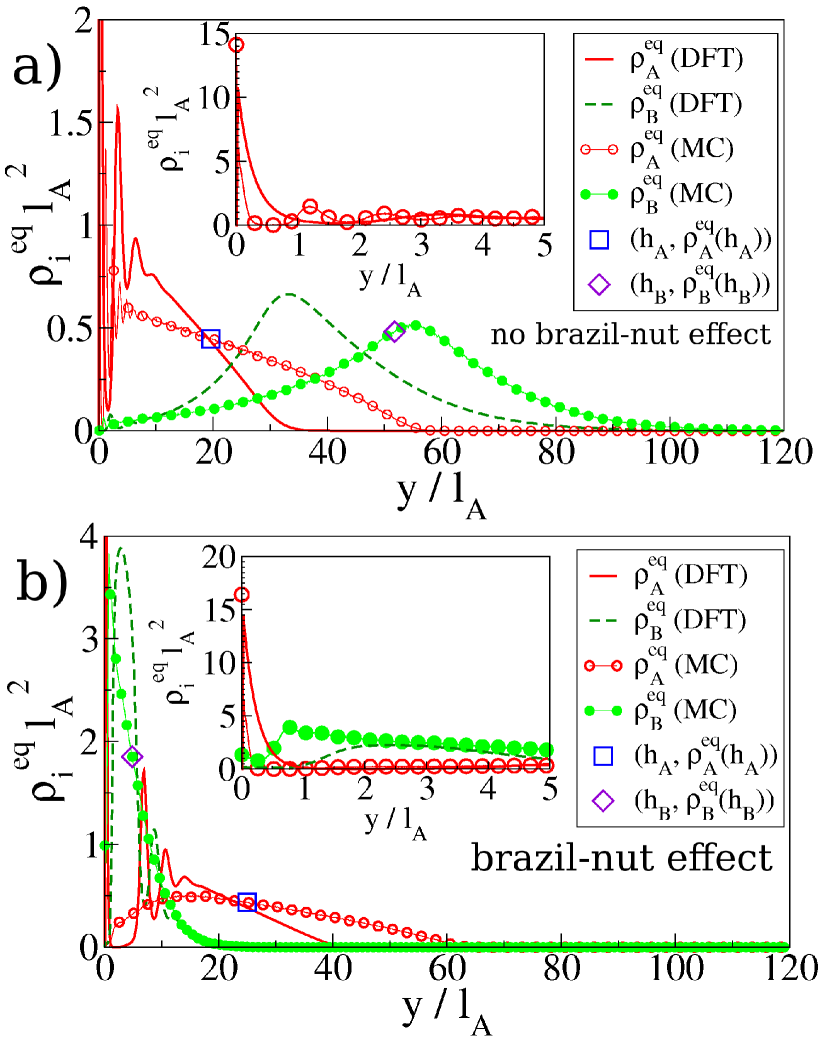
In order to quantify the colloidal brazil-nut effect, we follow the criterion proposed in Ref. Esztermann . We define averaged heights , by taking the first moment of the partial density fields as
| (14) |
In Fig. 1, the location of the corresponding heights are indicated by a large symbol. The brazil-nut effect is then defined by the condition
| (15) |
which means that on average, the heavier -particles are on top of the lighter -particles.
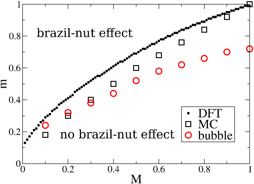
Within the full parameter range , , the region separating the brazil-nut effect from the ordinary behavior (no brazil-nut effect) is shown in Fig. 2. MC computer simulation data for the separation line are given by square symbols. These results were obtained by systematically scanning the parameter space. The brazil-nut effect occurs preferentially for strong dipolar asymmetry and is favoured if the two masses do not differ much. DFT results for the phase boundary are also included in Fig. 2 and are in good agreement with the simulation data predicting the same trends and the same slope of the separation line in the - parameter space.
IV.2 Depletion bubble picture
We now put forward an intuitive picture for the mechanism behind the colloidal brazil-nut effect which also provides a very simple theory for the separation line. This picture is based on the observation that when surrounded by a fluid of -particles, a single -particle creates a circular void-like space around it which is free of -particles due to the strong repulsion between - and -particles, see the highlighted area in Fig. 3. This depletion bubble is firmly attached to the -particle. Applying the buoyancy criterion to the whole bubble, the effective weight per area of the -particles is strongly reduced. Assuming a homogeneous fluid density surrounding a bubble of radius around an -particle, the brazil-nut condition for lifting the -particle can be stated as a buoyancy criterion
| (16) |
We estimate the radius by a low-density argument, where the density profile of -particles around an -particle fixed at the origin is such that a reasonable assumption for the radius of the depletion zone is given by the separation where the -interaction energy equals , i.e.
| (17) |
Upon insertion in Eqn. (16), this yields the brazil-nut condition
| (18) |
Thereby, a simple estimate for the separation line is provided. The only unknown parameter entering in Eqn. (18) is the averaged density . We have used simulation data to determine as the effective density at a distance :
| (19) |
The resulting separation line is included in Fig. 2. Despite its simplicity, the depletion bubble picture describes the simulation data pretty well.
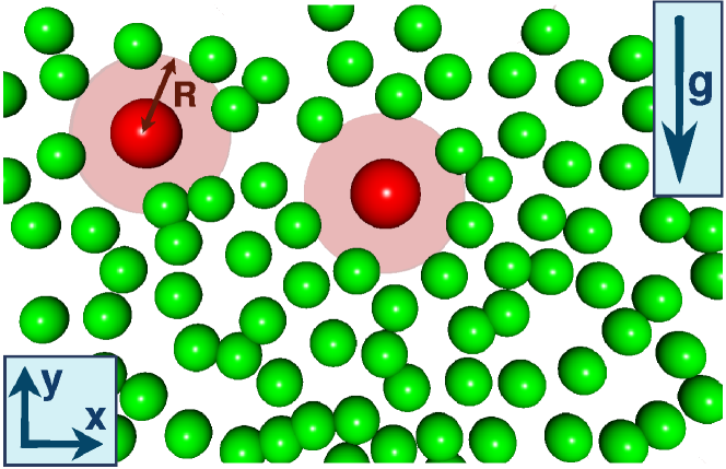
Clearly, the depletion bubble is induced by the soft long-ranged repulsion and is therefore missing for pure hard sphere mixtures where neighbouring particles are at contact. However, when the interaction is mapped onto a substitute interaction core with an effective diameter Roux_JPCM , all the traditional sedimentation is qualitatively contained in this effective hard sphere mixture.
IV.3 Boundary layering and effective interaction between an -particle and the bottom wall
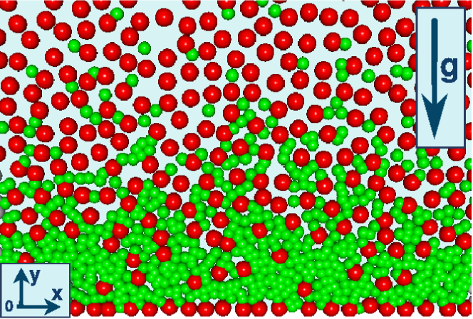
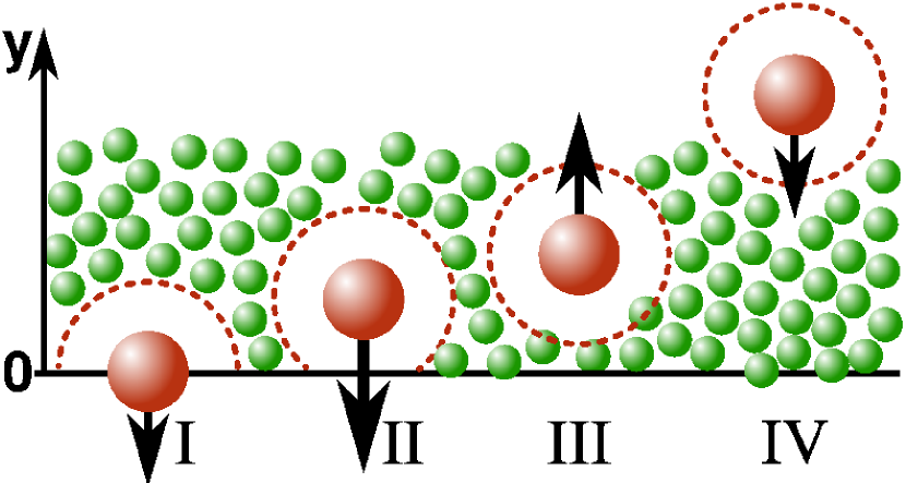
We finally discuss the implication of the depletion bubble on the layering of -particles close to the hard bottom wall of the confining container (at ), see again the insets of Fig. 1. The strong layering is clearly demonstrated by an actual simulation snapshot shown in Fig. 4.
If a single -particle is fixed at a given distance from the bottom wall, its depletion bubble is reduced since the void space is cut by the hard wall, see the sketch in Fig. 5. Note that the -particle is point-like so that in principle, it can approach the wall very closely. If the -particle is close to the wall, the void space is half of the full circle in the bulk (situations I and III in Fig. 5). If the height of the -particles increases, the depletion bubble area grows. Assuming a constant depletion bubble radius , is given analytically as
| (20) |
The growing bubble size causes two opposing effects: first, in order to increase the depletion bubble area, work against the osmotic pressure of the fluid -particles is necessary. Assuming that is constant in the small height regime, this work equals and gives rise to an effective attraction of an -particle close to the wall (situation II in Fig. 5). In fact, this attraction is similar to the depletion attraction in the ordinary Asakura-Oosawa-Vrij model of colloid-polymer mixtures near a hard wall Dijkstra ; Brader although there is a finite (physical) colloidal diameter in this model.
The second effect resulting from the increasing bubble size is a change in the effective buoyancy. The effective buoyant force is given by . If the bubble containing the -particle is lighter than the surrounding -fluid, this term is repulsive with respect to the wall and therefore opposed to the depletion force.
Combining these two effects, we gain the following analytical expression for the depletion potential between a single -particle and the wall:
| (21) |
where the integral can be calculated as
| (22) |
This expression requires as an input parameter. In order to evaluate , we have determined via a bulk reference simulation of a pure -system (in the absence of gravity) at a prescribed number density by using the virial expression Loewen1992 .
We further checked a posteriori whether the radius of the depletion bubble is consistent with that obtained from a radially averaged density profile of a bulk -fluid around a single -particle fixed at the origin. This ”renormalized” radius can be estimated to be the position of the first inflection point in this density profile of -particles (not shown here). Actually, we find values for which are a bit smaller than those given by the estimate (17) which only works at low .
More rigorously, we can define the effective interaction between the wall and an -particle under the presence of the inhomogeneous distribution of -particles by a potential of mean-force mcmillan1945 ; Hansen_Loewen . For a given altitude , the effective interaction potential is given by
| (23) |
where is the canonically averaged total force on the -particle in the presence of the -particles (which by symmetry points in the -direction). also contains the trivial direct part from gravity.
Computer simulation data for the effective potential are presented in Fig. 6.
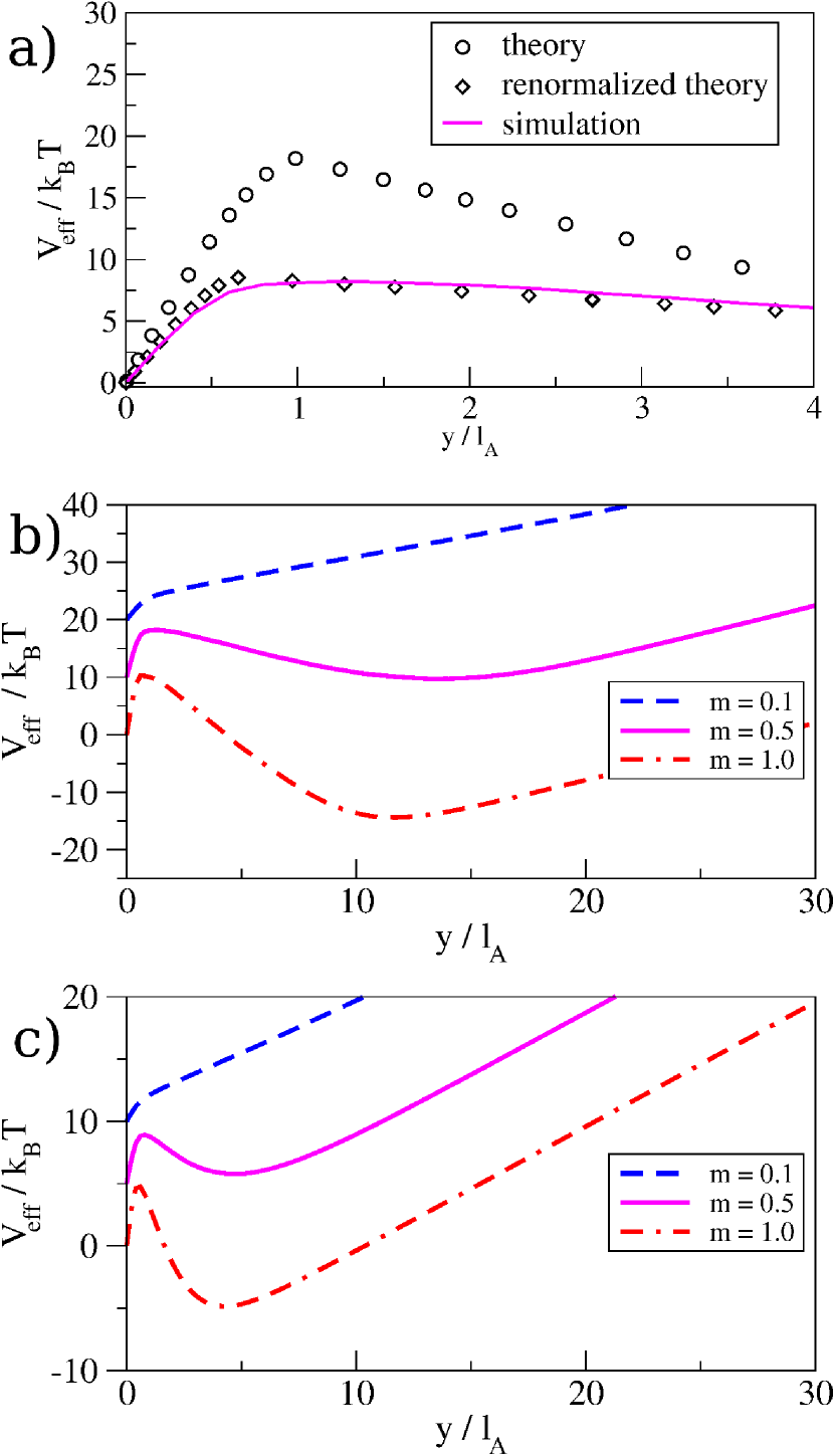
Two possibilities occur: if the -particle is much heavier than the -particles, the potential is fully attractive by a combination of depletion attraction close to the wall and gravity. In the brazil-nut case, on the other hand, there are three regimes in : an attractive regime close to the wall (corresponding to situation I,II in Fig. 5), followed by a repulsive regime (situation III in Fig. 5) and a subsequent attractive regime (situation IV in Fig. 5). The repulsive regime is caused by the lift force also responsible for the brazil-nut effect.
Fig. 6a includes the theoretical prediction of from Eqn. (21) for one set of parameters. There is very good agreement if the renormalized value for the depletion bubble radius is taken (diamonds) while the agreement deteriorates for the low-density-expression (circles). This demonstrates that the analytical expression (21) incorporates the basic physics principles.
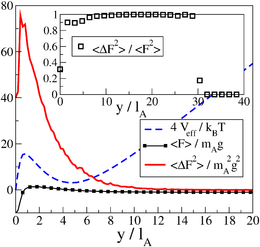
Between the short-ranged wall attraction and the lift regime, there is an energetic barrier typically of the order of several thermal energies . Comparing our MC simulation results to approximation (21) with renormalized bubble radius, the energetic barrier height proves to be in fair agreement. For , Eqn. (21) predicts , while we obtain from our MC simulation. Considering the parameter combination , an energetic barrier height follows from Eqn. (21), while MC simulation yields . Here, this large discrepancy can be attributed to the relatively thin layer of -particles close to the bottom wall.
If the energetic barrier is interpreted as a static one, an -particle which is initially trapped in the metastable minimum close to the wall needs a huge escape time to leave this metastable minimum which scales in an Arrhenius-like fashion . However, as pointed out by Vliegenthart et al. in Ref. vliegenthart2003 , the effective interaction can strongly fluctuate such that the energetic barrier is not static. In this case, the particle will escape much more quickly by waiting for a fluctuation which reduces the energetic barrier instantaneously and accelerates the escape process. Therefore, we have computed also the fluctuations of the depletion force , see Fig. 7. Near the potential barrier, increases significantly. The inset of Fig. 7 shows the relative fluctuations. They are indeed of the order one near the effective potential maximum. This indicates that -particles are exposed to strongly fluctuating forces when attempting to escape the boundary layer. Therefore, although the depletion potential comprises a potential barrier in the order of several , particle transitions from the boundary layer to higher altitudes occur at much higher frequencies than expected from the static activated Arrhenius expression . In fact, this facilitates the boundary layer sampling in the Monte-Carlo simulations of many -particles to a large extent and ensures sufficient equilibration.
V Results under time-dependent gravity (colloidal shaking)
Finally, we turn to the nonequilibrium situation of time-dependent gravity, see Eqn. 6, which is a simple model of colloidal shaking. As far as our methods are concerned, we now use Brownian dynamics simulations appropriate for colloids and dynamical density functional theory. Various different starting configurations were used in the simulations to obtain statistical averages which were all sampled from an interacting bulk system. This corresponds to an initial homogeneous density field in DDFT. The swap fraction is chosen to be , i.e. we consider the case that the time-average of the gravity is non-zero. In particular, we discuss the emergence of a steady state upon time-periodic gravity.
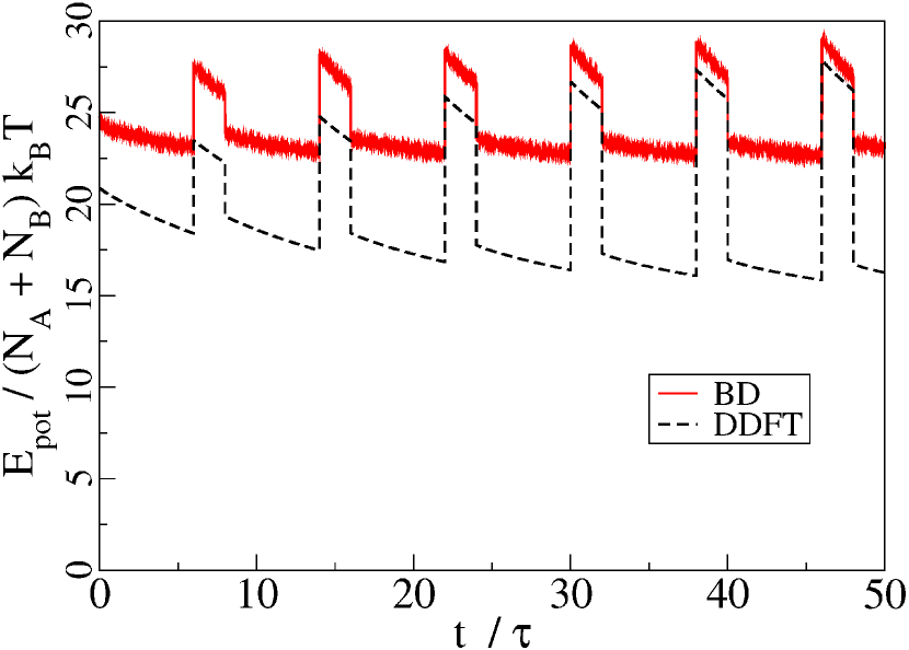
The relaxation of an initially homogeneous (but interacting) fluid of - and -particles towards its periodic steady state can be monitored by observing the instantaneous ensemble-averaged total potential energy of the system assoud2009 :
| (24) |
This quantity is shown in Fig. 8, indicating that only few oscillations are needed to get into the steady behavior. Due to the homogeneous starting configuration the energy oscillation amplitude increases with time. DDFT describes all trends correctly and also provides good data for the potential energies and the associated relaxation time.
The averaged height, as defined by the first moment of the density profile (see Eqn. (14)), can be generalized to a dynamical (time-dependent) quantity via
| (25) |
The time-dependent heights are another indicative parameter which probes the dynamical response of the whole system rex2008 ; rex2009 . The quantity is shown for two shaking frequencies in Fig. 9. As a result, the relaxation time is mainly scaling with the Brownian time but is rather insensitive to the periodicity . DDFT reproduces the trend with respect to increasing the periodicity but underestimates the actual heights , consistent with what we found in the equilibrium case.
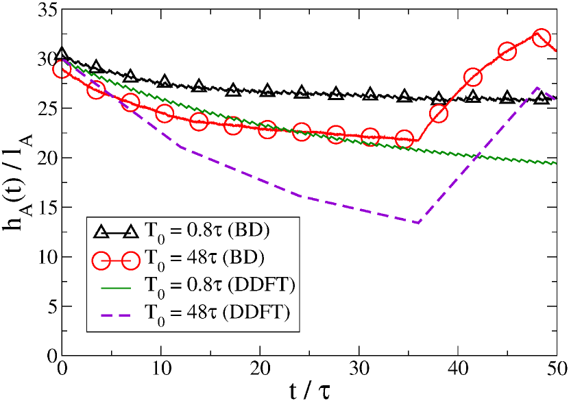
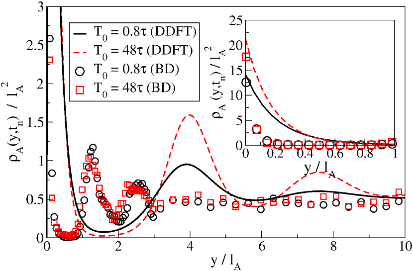
Upon shaking, the boundary layer of the -particles persists. We take a snapshot after the relaxation time at
| (26) |
This is just the time at which the direction of gravity is inverted. Comparing the results to the density profiles predicted by DDFT, the persistence of the boundary layer is indicated by both methods. Fig. 10 depicts density profiles obtained by BD simulations and DDFT for various shaking periods . Dynamical density functional data are in qualitative agreement with Brownian dynamics computer simulations results but show the same deficiencies as in the equilibrium case. This indicates that the deviations can be solely attributed to the quality of the density functional but not to the additional adiabatic approximation inherent in any DDFT. Again, as in equilibrium, the amplitude of the outermost density peak is in good agreement, see the inset of Fig. 10.
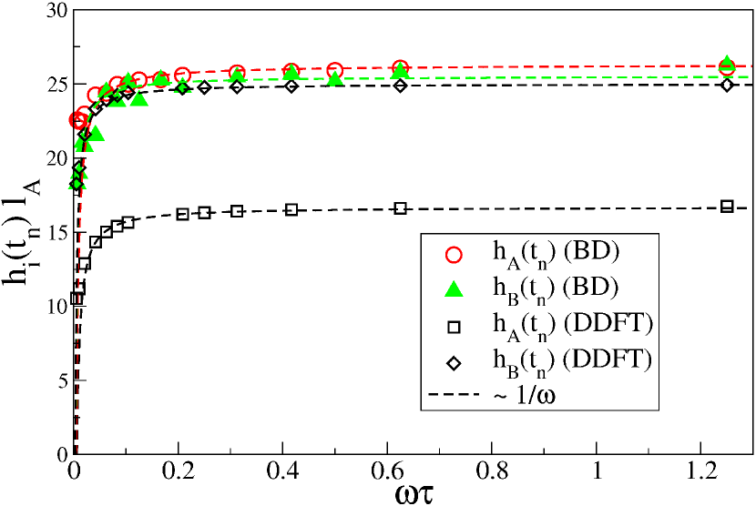
The mean heights at times are shown in Fig. 11 versus frequency . The dissipative response leads to a decay of the peak as a function of . For , we recover a quasi-static equilibrium case while for , the shaking is so fast that the system does not react at all upon this stimulus. It therefore approaches the limit of an ordinary equilibrium fluid mixture confined between two slits in the absence of gravity where layering is much less pronounced than in the presence of gravity. The crudest model of colloidal shaking is a completely overdamped response to a periodic external stimulus. In this case, the response amplitude scales with the shaking frequency as . A fit which involves the scaling is included in Fig. 11 and provides a good description in the high-frequency regime. The DDFT reproduces these trends and provides good data for while underestimating . Again, we attribute this to the low-density approximation of the functional, where the stronger interacting -particles are treated in a more approximative way than the -particles.
VI. CONCLUSIONS
In conclusion, we have explored a two-dimensional binary mixture of
particles interacting via long-ranged repulsive forces
in gravity by using computer simulation and density functional theory
theory. The
more repulsive -particles create a depletion zone (void space) of less
repulsive -particles around them
reminiscent to a bubble. Applying Archimedes’ principle effectively to this
bubble, an -particle can be lifted in a fluid background of
-particles. This mechanism also work when the -particles are heavier
than the -particles leading to a colloidal brazil
nut effect where the heavier particles float on top of the lighter
particles. Still the buoyancy principle is fulfilled
if it is effectively applied to the mass per bubble volume.
This general finding is
in accordance with the recent experimental sedimentation results on
colloidal mixtures by Serrano et al. Serrano .
Within the depletion bubble picture, an effective attraction of a -particles towards a hard container bottom wall is obtained which leads to boundary layering of the -particles. We have also studied a periodic inversion of gravity causing perpetuous mutual penetration of the mixture in a slit geometry. This non-equilibrium case of time-dependent gravity is similar to shaking. Upon shaking the boundary layering persists. Our results are based on Brownian dynamics computer simulations and density functional theory. The brazil-nut and boundary layering are very general effects, they do also occur for other long-ranged repulsive interactions and in three spatial dimensions. They are therefore verifiable in future settling experiments on dipolar or charged colloidal mixtures as well as in charged granulates and dusty plasmas.
Future work should address other interparticle interactions. Novel effects are expected for a strongly attractive cross-interactions leading to mutual mixing of - and -particles. These interactions are for example realized in oppositely charged suspensions leunissen2005 ; vissers2011 . It would be interesting to check whether a colloidal brazil-nut effect can still be observed in this case. Another option for future study is to superimpose more external fields (e.g. an external electric field) to the gravitational field in order to controll the response of the system even more hoffmann2000 . The latter set-up is relevant for electronic ink comiskey1998 ; gelinck2004 .
Acknowledgments
We thank M. Marechal for helpful discussions and L. Assoud for providing a computer code. This work was financially supported by the DFG within SFB TR6 (project C3).
References
- (1) A. Philipse, Current opinion in Colloid & Interface Science 2, 200 (1997).
- (2) V. Manoharan, M. Elsesser, and D. Pine, Science 301, 483 (2003).
- (3) M. Rasa and A. Philipse, Nature 429, 857 (2004).
- (4) A. Moncho-Jorda, A. Louis, and J. T. Padding, Phys. Rev. Lett. 104, 068301 (2010).
- (5) J. Williams, Powder Technol. 15, 245 (1976).
- (6) A. Rosato, K. Strandburg, F. Prinz, and H. Swendsen, Phys. Rev. Lett. 58, 1038 (1987).
- (7) T. Shinbrot and F. Muzzio, Phys. Rev. Lett. 81, 4365 (1998).
- (8) D. Hong, P. Quinn, and S. Luding, Phys. Rev. Lett. 86, 3423 (2001).
- (9) J. Both and D. Hong, Phys. Rev. Lett. 88, 124301 (2002).
- (10) A. Breu, H. Ensner, and C. Kruelle, Phys. Rev. Lett. 90, 014302 (2003).
- (11) S. Godoy, D. Risso, R. Soto, and P. Cordero, Phys. Rev. E 78, 031301 (2008).
- (12) V. Garzo, Phys. Rev. E 78, 020301 (2008).
- (13) A. Wysocki, C. P. Royall, R. Winkler, G. Gompper, H. Tanaka, A. van Blaaderen, and H. Löwen, Soft Matter 5, 1340 (2009).
- (14) H. Löwen, Soft Matter 6, 3133 (2010).
- (15) G. Brambilla, S. Buzzaccaro, R. Piazza, L. Berthier, and L. Cipelletti, Phys. Rev. Lett. 106, 118302 (2011).
- (16) C. Serrano, J. McDermott, and D. Velegol, Nature Mat. 10, 716 (2011).
- (17) T. Biben, R. Ohnesorge, and H. Löwen, Europhys. Lett. 28, 665 (1994).
- (18) K. Milinković, J. T. Padding, and M. Dijkstra, Soft Matter 7, 11177 (2011).
- (19) N. Lorenz, H. J. Schöpe, and T. Palberg, J. Chem. Phys. 131, 134501 (2009).
- (20) T. Okubo, A. Tsuchida, S. Takahashi, K. Taguchi, and M. Ishikawa, Coll. & Poymer Sci. 278, 202 (2000).
- (21) E. Vermolen, A. Kujik, L. Filion, M. Hermes, J. Thijssen, M. Dijkstra, and A. van Blaaderen, Proc. Nat. Acad. Sci. USA 106, 16063 (2009).
- (22) J. Gilchrist, A. Chan, E. Weeks, and J. Lewis, Langmuir 21, 11040 (2005).
- (23) A. Esztermann and H. Löwen, Europhys. Lett. 68, 120 (2004).
- (24) J. Zwanikken and R. van Roij, Europhys. Lett. 71, 480 (2005).
- (25) T. Biben and J.-P. Hansen, Mol. Phys. 80, 853 (1993).
- (26) J. Vesaratchanon, A. Nikolov, D. Wasan, and D. Henderson, Indust. Eng. Chem. Res. 48, 6641 (2009).
- (27) X. Chu, A. Nikolov, and D. Wasan, Chem. Eng. Comm. 150, 123 (1996).
- (28) M. Schmidt, M. Dijkstra, and J.-P. Hansen, Phys. Rev. Lett. 93, 088303 (2004).
- (29) M. Schmidt, M. Dijkstra, and J.-P. Hansen, J. Phys.: Condens. Matter 16, S4185 (2004).
- (30) C. P. Royall, J. Dzubiella, M. Schmidt, and A. van Blaaderen, Phys. Rev. Lett. 98, 188304 (2007).
- (31) J. P. Hoogenboom, D. Derks, P. Vergeer, and A. van Blaaderen, J. Chem. Phys. 117, 11320 (2002).
- (32) I. Ramsteiner, K. Jensen, D. Weitz, and F. Spaepen, Phys. Rev. E 79, 011403 (2009).
- (33) A. Mehrotra, S. Puri, and D. Khakhar, Phys. Rev. E 83, 061306 (2011).
- (34) M. Leocmach, C. P. Royall, and H. Tanaka, Europhys. Lett. 89, 38006 (2010).
- (35) B. Smorodin, B. Myznikova, and J. Legros, Phys. Fluids 20, 094102 (2008).
- (36) M. Kollmann, R. Hund, B. Rinn, G. Nägele, K. Zahn, H. König, G. Maret, R. Klein, and J. Dhont, Europhys. Lett 58, 919 (2002).
- (37) H. König, R. Hund, K. Zahn, and G. Maret, Eur. Phys. J. E 18, 287 (2005).
- (38) F. Ebert, P. Keim, and G. Maret, Eur. Phys. J. E 26, 161 (2008).
- (39) S. Mazoyer, F. Ebert, and P. Keim, Europhys. Lett. 88, 66004 (2009).
- (40) F. Ebert, G. Maret, and P. Keim, Eur. Phys. J. E 29, 311 (2009).
- (41) L. Assoud, F. Ebert, P. Keim, R. Messina, G. Maret, and H. Löwen, Phys. Rev. Lett. 102, 238301 (2009).
- (42) A. Pertsinidis and X. Ling, Nature 413, 147 (2001).
- (43) Z. Wang, A. Alsayed, A. Yodh, and Y. Han, J. Chem. Phys. 132, 154501 (2010).
- (44) M. C. Jenkins and S. Egelhaaf, J. Phys.: Condens. Matter 20, 404220 (2008).
- (45) A. Tilmatine, K. Medles, M. Younes, A. Bendaoud, and L. Dascalescu, IEEE Trans. Ind. Appl. 48, 1564 (2010).
- (46) V. Tsytovich, G. Morfill, U. Konopka, and H. Thomas, New J. Phys. 5, 66 (2003).
- (47) G. Morfill and A. Ivlev, Rev. Mod. Phys. 81, 1353 (2009).
- (48) L. Assoud, F. Ebert, P. Keim, R. Messina, G. Maret, and H. Löwen, Phys. Rev. Lett. 102, 238301 (2009).
- (49) J.-P. Hansen and I. MacDonald, Theory of simple liquids (Academic, London, ADDRESS, 1976).
- (50) M. Allen and D. Tildesley, Computer simulation of liquids (Clarendon, Oxford, 1989).
- (51) T. Stirner and J. Sun, Langmuir 21, 6636 (2005).
- (52) D. Frenkel and B. Smit, Understanding Molecular Simulation (Academic Press, San Diego, ADDRESS, 2001).
- (53) N. Mermin, Phys. Rev. 137, A1441 (1965).
- (54) D. Evans, Adv. Phys. 51, 1529 (2002).
- (55) H. Löwen, Phys. Rep. 237, 249 (1994).
- (56) L. Onsager, Ann. N. Y. Acad. Sci. 51, 627 (1949).
- (57) H. H. Wensink and H. Löwen, Phys. Rev. E 78, 031409 (2008).
- (58) Y. Rosenfeld, M. Schmidt, H. Löwen, and P. Tarazona, Phys. Rev. E 55, 4245 (1997).
- (59) M. Oettel, s. Görig, and A. Härtel, Phys. Rev. E 82, 051404 (2010).
- (60) A Ramakrishnan-Yussouff approximation was put forward for one-component dipoles in S. van Teeffelen, N. Hoffmann, C. N. Likos, H. Löwen, Europhysics Letters 75, 583-589 (2006), but this was never generalized to repulsive mixtures.
- (61) U. Marconi and P. Tarazona, J. Chem. Phys. 110, 8032 (1999).
- (62) A. Archer and R. Evans, J. Chem. Phys. 121, 4246 (2004).
- (63) P. Español and H. Löwen, J. Chem. Phys. 131, 244101 (2009).
- (64) M. Heni and H. Löwen, Phys. Rev. Lett. 85, 3668 (2000).
- (65) The opposite case (for ) where the weaker coupled particles are heavier is not considered in this paper though it is in principle realizable.
- (66) H. Löwen, J. Roux, and J.-P. Hansen, J. Phys.: Condens. Matter 3, 997 (1991).
- (67) J. Brader, M. Dijkstra, and R. Evans, Phys. Rev. E 63, 041405 (2001).
- (68) J. Brader, R. Evans, and M. Schmidt, J. Phys.: Condens. Matter 14, L1 (2002).
- (69) H. Löwen, J. Phys.: Condens. Matter 4, 10105 (1992).
- (70) W. McMillan and J. Mayer, J. Chem. Phys. 13, 276 (1945).
- (71) J.-P. Hansen and H. Löwen, Ann. Rev. Phys. Chem. 51, 209 (2000).
- (72) G. Vliegenthart and P. van der Schoot, Europhys. Lett. 62, 600 (2003).
- (73) M. Rex and H. Löwen, Phys. Rev. Lett. 101, 148302 (2008).
- (74) M. Rex and H. Löwen, Eur. Phys. J. E 28, 139 (2009).
- (75) M. Leunissen, C. Christova, A.-P. Hynninen, C. P. Royall, A. Campbell, A. Imhof, M. Dijkstra, R. van Roij, and A. van Blaaderen, Nature 437, 235 (2005).
- (76) T. Vissers, A. Wysocki, M. Rex, H. Löwen, C. P. Royall, A. Imhof, and A. van Blaaderen, Soft Matter 7, 2352 (2011).
- (77) G. Hoffmann and H. Löwen, J. Phys.: Condens. Matter 12, 7359 (2000).
- (78) B. Comiskey, J. Albert, H. Yoshizawa, and J. Jacobson, Nature 394, 253 (1998).
- (79) G. Gelinck, H. Huitema, E. Van Veenedaal, E. Cantatore, L. Schrijnemakers, J. Van der Putten, T. Geuns, M. Beenhakkers, J. Giesbers, B. Huisman, E. Meijer, E. Benito, F. Touwslager, A. Marsman, B. Van Rens, and D. De Leeuw, Nature Mat. 3, 106 (2004).