Quenching across quantum critical points in periodic systems: dependence of scaling laws on periodicity

Abstract

We study the quenching dynamics of a many-body system in one dimension described by a Hamiltonian that has spatial periodicity. Specifically, we consider a spin-1/2 chain with equal $xx$ and $yy$ couplings and subject to a periodically varying magnetic field in the $\hat{z}$ direction or, equivalently, a tight-binding model of spinless fermions with a periodic local chemical potential, having period $2q$, where $q$ is a natural number. For a linear quench of the magnetic field strength (or potential strength) at rate $1/\tau$ across a quantum critical point, we find that the density of defects thereby produced scales as $1/\tau^{q/(q+1)}$, deviating from the $1/\sqrt{\tau}$ scaling that is ubiquitous to a range of systems. We analyze this behavior by mapping the low-energy physics of the system to a set of fermionic two-level systems labeled by the lattice momentum $k$ undergoing a non-linear quench as well as by performing numerical simulations. We also find that if the magnetic field is a superposition of different periods, the power law depends only on the smallest period for very large values of $\tau$ although it may exhibit a cross-over at intermediate values of $\tau$. Finally, for the case where a $zz$ coupling is also present in the spin chain, or equivalently, where interactions are present in the fermionic system, we argue that the power associated with the scaling law depends on a combination of $q$ and interaction strength.

I Introduction

The quenching dynamics of quantum many-body systems has become a topic of active research in recent years kibble ; zurek ; polkov05 ; calabrese ; levitov ; dutta ; singh ; mondal1 ; mondal2 ; polkov08 ; patane ; degrandi ; bermudez ; vish ; pollmann ; dziarmaga . In particular, there has been a focus on the effects of slow quenching across a quantum critical point (QCP). Here a parameter $\lambda$ in the Hamiltonian describing a quantum system is varied linearly (for instance) in time at a rate given by $1/\tau$, such that the system starts in the ground state far away on one side of a QCP, crosses the QCP at a critical parameter value $\lambda_{c}$, and ends far away on the other side of the QCP. The final state of the system is in fact dominated by the regime close to the QCPkibble ; zurek ; polkov05 where the correlation length of the system diverges as $|\lambda-\lambda_{c}|^{-\nu}$ and the relaxation time (or the inverse of the energy gap between the ground state and the first excited state) diverges as $|\lambda-\lambda_{c}|^{-z\nu}$. No matter how small the quenching rate $1/\tau$, the relaxation time for the system is larger than $\tau$ because at the QCP, there exist modes with energies arbitrarily close to zero. The quenching process near $\lambda_{c}$ is not adiabatic for such modes, and the system does not reach the ground state of the final Hamiltonian. The final state contains a finite density of defects which scales as a power of $\tau$ for small $1/\tau$ given by the Kibble-Zurek (KZ) form $1/\tau^{d\nu/(z\nu+1)}$. The power thus depends on only three quantities; the spatial dimensionality $d$, and critical exponents $\nu$ and $z$. For a large class of translationally invariant systems, the Hamiltonian decouples into several pairs of momentum modes of opposite sign. In such systems, quenching dynamics and power-law scaling can be analyzed by mapping the problem to the dynamics of the Landau-Zener transition of a two-level system dictated by a time-dependent tuning parameter zurek . In several such instances in one dimension, one has $z=\nu=1$, giving rise to the ubiquitous $1/\tau^{1/2}$ scaling of the density of defects scales.

While the above scaling law holds for a range of systems, some generalizations and deviations thereof are coming to light. For instance, if the Hamiltonian is varied across the QCP non-linearly in time, as $(t/\tau)^{\alpha}$, the scaling law becomes $1/\tau^{d\nu\alpha/(z\nu\alpha+1)}$ mondal2 ; polkov08 . Effectively, the non-linear quench modifies the exponent $\nu$ to $\nu\alpha$. As another instance, it has also been shown that the power law can depend on certain topological features of the system bermudez ; vish ; wade . In particular, in Refs. vish, and wade, , some of the authors of the present work have studied quenching dynamics in a two-legged ladder version of the Kitaev model. As with the parent Kitaev model on the hexagonal lattice kitaev ; feng ; nussinov , the two-legged ladder has a large number of sectors (growing exponentially with the number of sites) which are distinguished by the eigenvalues ($\pm 1$) of a number of local $Z_{2}$-valued conserved quantities feng ; vish . The ladder was mapped to a fermionic $p$-wave superconducting system which has recently emerged as an exciting topological system in its own right hasan . It was shown that while quenching through QCPs in certain sectors yields the standard $1/\tau^{1/2}$ scaling of the defect density (also related to the total probability of excitations), certain periodic patterns in the $Z_{2}$ invariants give rise to a $1/\tau^{2/3}$ scaling. It was further conjectured in Ref. vish, that more general scaling laws of the form $1/\tau^{q/(q+1)}$ for the slew of integers $q=3,4,\cdots$ may appear in some other sectors, but explicit examples of such sectors were not found in that model.

In this work, we show that the presence of a periodically varying parameter in an otherwise spatially homogeneous system provides an excellent route for new and interesting power-law quenching behavior, inclusive of the $1/\tau^{q/(q+1)}$ scaling. We demonstrate the role of periodicity in the specific case of a one-dimensional spin-1/2 lattice model having homogeneous and equal nearest-neighbor $xx$ and $yy$ couplings and subject to a transverse periodically varying magnetic field having the value $h\cos(Qn+\phi)$ at site $n$. By the Jordan-Wigner transformation, we equivalently study a tight-binding system of non-interacting spinless fermions in one dimension in which the local chemical potential varies as $h\cos(Qn+\phi)$. For $Q=\pi/q$ (where $q=1,2,\cdots$), the system exhibits a spatial periodicity of $2q$, fragmenting the Brillouin zone into $2q$ regions that are coupled to one another by the periodic potential. In contrast to the aforementioned case of pairwise coupling of modes of opposite momentum, the periodicity presents a more complex structure in which a quench can cause probability amplitudes to shift between these $2q$ modes. While the total post-quench excitation probability is still dominated by the QCP at $h=0$ and the gapless points at momenta $k=\pm\pi/2$, it depends on the intermediate paths taken by the matrix elements connecting the various fragments of the Brillouin zone; the parameter $\phi$ controls the relative phase between the different paths. Using perturbation theory to $q$-th order for small $h$, we explicitly illustrate this point for a linear quench where the amplitude $h$ varies linearly in time as $t/\tau$ so as to go from $-\infty$ to $\infty$. The perturbation provides an effective low-energy Hamiltonian for momentum modes around $k=\pm\pi/2$ and reduces the dynamics to the generalized Landau-Zener evolution of a set of two-level systems in the presence of a $|t/\tau|^{q}$ time variation, reminiscent of the non-linear $t^{\alpha}$ quench. The behavior of $p_{k}$, the excitation probability for each momentum mode, becomes increasingly complex as the value of $q$ increases; however, a simple scaling analysis shows that the total excitation probability only gets a contributions from modes lying within a range of $k$ given by $\Delta k\sim(\cos(q\phi)/\tau^{q})^{1/(q+1)}$ or $(\sin(q\phi)/\tau^{q})^{1/(q+1)}$, depending on whether $q$ is odd or even, respectively. Hence the total excitation probability for the quench yields the desired $1/\tau^{q/(q+1)}$ scaling law, multiplied by $(\cos(q\phi))^{1/(q+1)}$ or $(\sin(q\phi))^{1/(q+1)}$. We corroborate and expand our analytical arguments using numerics. It turns out that one can think of the effective low-energy theory as either describing a system with $\nu=1$ and a Hamiltonian varying in time with a power $\alpha=q$, or as a system with $\nu=q$ with a Hamiltonian varying linearly in time ($\alpha=1$). In all cases, we obtain a KZ power law of the form $1/\tau^{d\nu\alpha/(z\nu\alpha+1)}$, where $d=1$, $z=1$, and $\nu\alpha=q$.Our results thus show that internal mode structure, when combined with critical behavior and quenching, can give rise to rich out-of-equilibrium dynamics and scaling.

In another line of investigation, it has been shown that the simple post-quench $1/\sqrt{\tau}$ scaling can have drastic modifications due to a completely different reason, namely, interactionsdegrandi ; pollmann . In Ref. degrandi, , an interacting system of bosons in the presence of a periodic potential permitting one boson per potential minimum was analyzed within a sine-Gordon framework. It was shown that a quench in the strength of the periodic potential results in the density of defects having a power law scaling with an exponent that depends explicitly on the interaction strength. In the context of our work, interactions in a sense are an extreme limit of coupling between momentum modes. Borrowing from the analysis of Ref. degrandi, , we extend our studies of periodic structures to include interactions in our fermionic system, or equivalently, to include a $zz$ coupling in the spin chain system. We argue that the scaling exponent for the total excitation probability now depends on both interactions and the periodicity $q$ and that this result is also valid for a generalization of the studies in Ref. degrandi, to the case of $q$ bosons per potential minimum.

We present our studies as follows. In Sec. II, we introduce the spin and fermion models, express the periodic term in the basis of Brillouin zone modes and derive the effective low energy Hamiltonian using perturbation theory. In Sec. III, we analytically derive the scaling behavior of the system for a linear quench in $h$ and present numerical results of quenching simulations for different values of $q$, phase $\phi$ and quenching rate $1/\tau$. To understand the detailed dependence of $p_{k}$ on $k$, we study in the Appendix a two-level problem in which the time-dependent term in the Hamiltonian as $|t|^{q}sgn(t)$ (where $sgn$ denotes the signum function). In Sec. IV, we study more complex behavior of the periodic potential such as a superposition of two commensurate periodic functions; we find that the power law scaling for the total excitation probability is governed by the smallest period for very large values of $\tau$ although the power law may show a cross-over at intermediate values of $\tau$. In Sec. V we consider the effect of interactions and we conclude with general remarks in Sec. VI.

II The model and its energy spectrum

Our starting point is a one-dimensional spin-1/2 model placed in a transverse magnetic field whose Hamiltonian is given by

$$H~{}=~{}-J~{}\sum_{n=-N}^{N}~{}[~{}\sigma_{n}^{x}\sigma_{n+1}^{x}~{}+~{}\sigma_{n}^{y}\sigma_{n+1}^{y}~{}+~{}h_{n}\sigma_{n}^{z}~{}],$$ (1)

where $\sigma_{n}^{\alpha}$ ($\alpha=x,y,z$) denote the Pauli matrices at site $n$, and we are eventually interested in the thermodynamic limit $N\to\infty$. (We generally set $\hbar$, the exchange coupling $J$ and the lattice spacing $a$ equal to unity. When we introduce a quenching time $\tau$, large or small values of $\tau$ are as compared to $\hbar/J$.) Note that $\sum_{n}\sigma_{n}^{z}$ commutes with the Hamiltonian. This system can be mapped to a model of spinless fermions using the Jordan-Wigner transformation lieb61 . At any site $n$, we map a spin state with $\sigma_{n}^{z}=1$ or $\sigma_{n}^{z}=-1$ to the presence or absence of a spinless fermion at that site; this is done by introducing a fermion annihilation operator $c_{n}$ at each site, and writing the spin at that site as

$$\sigma_{n}^{z} = 2c_{n}^{\dagger}c_{n}-1=2\rho_{n}-1$$

$$\sigma_{n}^{-} = \frac{1}{2}(\sigma_{n}^{x}-i\sigma_{n}^{y})=c_{n}~{}e^{i\pi\sum_{j=-N}^{n-1}c_{j}^{\dagger}c_{j}},$$ (2)

where $c_{j}^{\dagger}c_{j}=0$ or 1 is the fermion occupation number at site $j$. The expression for $\sigma_{n}^{+}$ can be obtained by taking the Hermitian conjugate of $\sigma_{n}^{-}$. The string factor in the definition of $\sigma_{n}^{-}$ is necessary to ensure the correct anticommutation relations between the fermionic operators, namely, $\{c_{m},c_{n}^{\dagger}\}=\delta_{mn}$ and $\{c_{m},c_{n}\}=0$.

[In this paper, we will use both first quantized notation (wave functions) and second quantized notation (fermion creation and annihilation operators and occupation number basis) as per convenience We specify the notation being used where necessary.]

Following the Jordan-Wigner transformation, Eq. (1) takes the form

$$H~{}=~{}-\sum_{n=-N}^{N}~{}[2(c_{n}^{\dagger}c_{n+1}+c_{n+1}^{\dagger}c_{n})~{}+~{}2h_{n}~{}c_{n}^{\dagger}c_{n}],$$ (3)

where we have omitted a constant equal to $\sum_{n}h_{n}$. The fermionic operators can be represented in the momentum basis by the Fourier transform

$$c_{k}~{}=~{}\frac{1}{\sqrt{2N+1}}~{}\sum_{n=-N}^{N}c_{n}e^{-ikn},$$ (4)

where the momentum $k$ lies in the range $[-\pi,\pi]$ and is quantized in units of $2\pi/(2N+1)$; these operators satisfy the anti-commutation rules $\{c_{k},c_{k^{\prime}}^{\dagger}\}=\delta_{k,k^{\prime}}$. In momentum space, the first two terms of the Hamiltonian in Eq. (3) have the tight-binding form

$$H_{0}~{}=~{}-\sum_{-\pi<k\leq\pi}~{}4\cos(ka)~{}c_{k}^{\dagger}c_{k}.$$ (5)

As for the last term in Eq. (3), we consider the situation where $h_{n}=h\cos(Qn+\phi)$. We note that this Hamiltonian appears in the Azbel-Hofstadter problemazbel of an electron hopping between the sites of a square lattice in the presence of a magnetic field applied in the perpendicular direction; the magnetic flux per square is proportional to $Q$. This problem has been studied extensively, and we will refer to only some of the papers here hsu ; sen00 .

For the case $Q=\pi/q$, where $q$ is an integer, the periodicity of the magnetic field is $2q$. Using the decomposition

$$h_{n}~{}=~{}\frac{h}{2}~{}(e^{i(\pi n/q+\phi)}~{}+~{}e^{-i(\pi n/q+\phi)}),$$ (6)

we see that this term couples two fermionic modes with momenta $k_{1}$ and $k_{2}$ if $k_{1}=k_{2}\pm\pi/q$. This periodic term fragments the Hamiltonian into a $2q$ dimensional matrix form composed of momentum regions $-\pi+r\pi/q<k\leq-\pi+(r+1)\pi/q$ with $0\leq r\leq 2q-1$. The tight-binding term of Eq. (3) is diagonal in this basis while the periodic potential connects neighboring momentum regions. The corresponding matrix elements of $H_{k}$ are given by

$$\langle k+r\pi/q|H_{k}|k+s\pi/q\rangle$$

$$=-4\cos(k+s\pi/q)~{}\delta_{r,s}-he^{i\phi}~{}\delta_{r,s+1}-he^{-i\phi}~{}\delta_{r,s-1},$$

(7)

where $0\leq r,s\leq 2q-1$, and we have assumed ‘periodic boundary conditions’ for the matrix $H_{k}$, so that $r=-1$ and $2q$ mean $r=2q-1$ and $0$ respectively. We have thus reduced Eq. (3) to the decoupled form

$$H~{}=~{}\sum_{k=-\pi}^{-\pi+\pi/q}~{}H_{k}.$$ (8)

Note that the total fermion number ${\cal N}=\sum_{n=-N}^{N}c_{n}^{\dagger}c_{n}=\sum_{k=-\pi}^{\pi}c_{k}^{\dagger}c_{k}$ commutes with each of the $H_{k}$ and is therefore conserved in time.

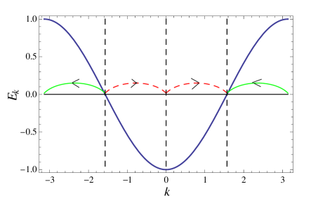
Figure 1: Picture of intermediate states for the case $q=2$. The zero energy states at momenta $k=\pm\pi/2$ are connected to each other through the states lying at $k=0$ and $\pi$, as shown by red (dashed) and green (solid) lines respectively; the dispersion relation $E_{k}=-\cos k$ is indicated by a thick solid line. The system is described by a set of decoupled Hamiltonians $H_{k}$ labeled by $k$ lying in the range $[-\pi,-\pi/2]$; each $H_{k}$ is a four-dimensional matrix in which the momenta $k$, $k+\pi/2$, $k+\pi$ and $k+3\pi/2$, lying in the regions separated by the vertical dotted lines, are coupled to each other.

We now consider the energy spectrum of $H_{k}$, focusing on the low energy excitations that give the dominant contribution to the quench. As will be discussed in Sec. III, the initial condition for the quenching dynamics is such that the system is at half-filling at all times; we will therefore be particularly interested in the states near zero energy which correspond to the momenta $k=\pm k_{F}$, where the Fermi momentum $k_{F}=\pi/2$. If the amplitude $h$ of the magnetic field is zero, the system is gapless and the states at $k=\pm\pi/2$ are degenerate with each other. A small, non-vanishing value of $h$ (compared with the bandwidth) breaks this degeneracy in a manner that we derive using a perturbative expansion in $h$. To consider coupling between the $k=-\pi/2$ and $k=\pi/2$ regions, one can go through one series of intermediate states lying at $k=-\pi/2+\pi/q$, $-\pi/2+2\pi/q$, $\cdots$, $\pi/2-\pi/q$ (with an amplitude equal to $-he^{i\phi}$ at each step), and through another series of intermediate states lying at $k=-\pi/2-\pi/q$, $-\pi/2-2\pi/q$, $\cdots$, $\pi/2+\pi/q$ (with an amplitude equal to $-he^{-i\phi}$ at each step). A picture of these two series of intermediate states is shown in Fig. 1 for $q=2$. Each of these series consists of $q-1$ intermediate states. At the $q$-th order in perturbation theory, we therefore obtain an effective Hamiltonian $H_{eff}$ which has a matrix element between the states at $k=\pm\pi/2$ given by

$$\Delta\equiv\langle\pi/2|H_{eff}|-\pi/2\rangle~{}=~{}\langle-\pi/2|H_{eff}|\pi/2\rangle^{*}$$

$$=~{}\frac{(-he^{i\phi})^{q}}{\prod_{s=1}^{q-1}~{}(4\cos(-\pi/2+s\pi/q))}$$

$$~{}+~{}\frac{(-he^{-i\phi})^{q}}{\prod_{s=1}^{q-1}~{}(4\cos(-\pi/2-s\pi/q))},$$ (9)

where the denominators come from factors like $E_{-\pi/2}-E_{-\pi/2\pm s\pi/q}=4\cos(-\pi/2+\pm s\pi/q)$ corresponding to the energies in the unperturbed Hamiltonian in Eq. (5).

Simplifying Eq. (9) gives

$$\Delta=\langle\pi/2|H_{eff}|-\pi/2\rangle~{}=~{}\langle-\pi/2|H_{eff}|\pi/2\rangle^{*}$$

$$=~{}(-1)^{q}h^{q}~{}\frac{e^{iq\phi}+(-1)^{q-1}e^{-iq\phi}}{\prod_{s=1}^{q-1}~{}(4\sin(\pi s/q))}.$$ (10)

We thus find that the magnitude of $\Delta$ is given by

$$|\Delta| = \frac{h^{q}}{4^{q-1}}~{}\frac{2|\cos(q\phi)|}{\prod_{s=1}^{q-1}~{}\sin(\pi s/q)}~{}~{}~{}{\rm if}~{}~{}q~{}{\rm~{}is~{}odd},$$ (11)

$$= \frac{h^{q}}{4^{q-1}}~{}\frac{2|\sin(q\phi)|}{\prod_{s=1}^{q-1}~{}\sin(\pi s/q)}~{}~{}~{}{\rm if}~{}~{}q~{}{\rm~{}is~{}even}.$$

In a sense, the phase $\phi$ governs the relative phase between the two paths of intermediate states which connect the low lying states. We assume here that $\phi$ is such that $\cos(q\phi)\neq 0$ if $q$ is odd, and $\sin(q\phi)\neq 0$ if $q$ is even; if these conditions are violated, we would have to go to higher order perturbation theory to find a non-zero matrix element connecting the states at $k=\pm\pi/2$.

We can now consider moving slightly away from $k=\pm\pi/2$; then the unperturbed energies of the states $k=-\pi/2+k^{\prime}$ and $\pi/2+k^{\prime}$ are given by $-4k^{\prime}$ and $4k^{\prime}$ respectively. The effective Hamiltonian describing these two states is then given by the $2\times 2$ matrix

$$H_{eff,k^{\prime}}~{}=~{}\left(\begin{array}[]{cc}-4k^{\prime}&\Delta^{*}\\ \Delta&4k^{\prime}\end{array}\right),$$ (12)

where we assume that $\Delta$ continues to be given by the expression in Eq. (10) because $k^{\prime}$ is small. The eigenvalues of (12) are given by $\pm\sqrt{(4k^{\prime})^{2}+|\Delta|^{2}}$; this is the dispersion of a massive relativistic particle whose velocity is equal to the Fermi velocity $v_{F}=4$ and mass is proportional to $|\Delta|\sim h^{q}$ times $\cos(q\phi)$ or $\sin(q\phi)$.

Hence, $h=0$ corresponds to a QCP where the mass gap vanishes. Given that the energy vanishes as $|k^{\prime}|$ if $h=0$ and as $h^{q}$ if $k^{\prime}=0$, the dynamical critical exponent and correlation length exponent are given by $z=1$ and $\nu=q$, respectively. The correlation length exponent $\nu$ thus depends on the periodicity of the magnetic field $h_{n}$.

III Quenching dynamics

Having established the form of the Hamiltonian for the periodic system and its effective low-energy description, we now consider a specific quenching protocol.Given the magnetic field $h_{n}=h\cos(\pi n/q+\phi)$, we vary the amplitude of the field in time as $h=t/\tau$, where we refer to $\tau$ as the quenching time. At $t=-\infty$ ($h=-\infty$), we start with the ground state of the Hamiltonian denoted by $\Psi_{0}(-\infty)$. (Throughout this section, the symbol $\Psi$ denotes first quantized wave functions). $\Psi_{0}(-\infty)$ is the state in which $\sigma_{n}^{z}=1$ ($c_{n}^{\dagger}c_{n}=1$) at all the sites where $\cos(\pi n/q+\phi)>0$, and $\sigma_{n}^{z}=-1$ ($c_{n}^{\dagger}c_{n}=0$) at all the sites where $\cos(\pi n/q+\phi)<0$. [If $\cos(\pi n/q+\phi)=0$ for some value of $n$, the ground state is not unique in the limit $h=-\infty$, since the states with $c_{n}^{\dagger}c_{n}=0$ and 1 are then degenerate. We therefore assume that $\cos(\pi n/q+\phi)\neq 0$ for all values of $n$ and that a finite number of values of $\phi$ are avoided. This is equivalent to the conditions imposed on $\cos(q\phi)$ or $\sin(q\phi)$ after Eq. (11).] It is clear that in the range $1\leq n\leq 2q$, $\cos(\pi n/q+\phi)$ is positive for half the sites and negative for the other half. Hence, the ground state is half-filled in terms of fermions. We can write the ground state as the product of ground states of the $2q$-dimensional Hamiltonians $H_{k}(h=-\infty)$,

$$\Psi_{0}(-\infty)=\bigotimes\Psi_{0,k}(-\infty),$$ (13)

where $\Psi_{0,k}(-\infty)$ is a first quantized wave function which is obtained as follows. In the limit $h\to-\infty$, the on-site term is much larger than the hopping term in Eq. (3); hence the Hamiltonian $H_{k}$ becomes independent of $k$ in this limit. This implies that since the ground state is half-filled in real space, the states corresponding to the wave function $\Psi_{0,k}(t\to-\infty)$ are also half-filled for each value of $k$. Thus $\Psi_{0,k}(t\to-\infty)$ denotes the wave function corresponding to the state in which the $q$ negative energy states of $H_{k}(h=-\infty)$ are occupied by fermions and the $q$ positive energy states of $H_{k}(h=-\infty)$ are empty.

The system evolves dynamically according to the time-dependent Schrödinger equation. The state at time $t$ is once again given by a product

$$\Psi(t)=\bigotimes\Psi_{k}(t),$$ (14)

where the first quantized wave function $\Psi_{k}(t)$ is obtained by using $H_{k}(t)$ for the time evolution. In the limit $t\to\infty$ ($h\to\infty$), we reach the state $\Psi(\infty)=\bigotimes\Psi_{k}(\infty)$. Since the Hamiltonian changes time at a finite rate $1/\tau$, we expect that $\Psi(\infty)$ will differ from the ground state of the final Hamiltonian, $\Psi_{0}(\infty)=\bigotimes\Psi_{0,k}(\infty)$ except in the adiabatic limit. Our goal is to determine how far $\Psi(\infty)$ is from the final ground state $\Psi_{0}(\infty)$ as a function of $\tau$, quantifiable by the total excitation probability $P$. [Note that the final ground state $\Psi_{0}(\infty)$ is also half-filled; indeed this is the reason for choosing $h_{n}$ to have an even period, $2q$, so that both the initial ground state and the final ground state have the same filling. If the period of $h_{n}$ were odd, the initial and final ground states, corresponding to $h=-\infty$ and $\infty$, respectively, would have different occupation numbers, and it would not be possible for $\Psi_{0}(-\infty)$ to evolve in time to $\Psi_{0}(\infty)$ even in the limit $\tau\to\infty$, since the dynamics conserves the fermion number].

The formal procedure for evaluating the final state, as employed in our numerical calculations is as follows. We define a $2q$-dimensional matrix $M$ whose elements are given by

$$M_{rs}~{}=~{}e^{i\phi}~{}\delta_{r,s+1}~{}+~{}e^{-i\phi}~{}\delta_{r,s-1}$$ (15)

for $0\leq s\leq 2q-1$, and we again assume ‘periodic boundary conditions’ for the matrix $M$. In the limit $h\to-\infty$, the magnetic term dominates the system and the eigenvalues of the matrix $H_{k}$ in Eq. (7) are the same as those of $M$, while in the limit of $h\to\infty$, the eigenvalues of $H_{k}$ are the same as those of $-M$. Let the $q$ eigenvectors of $M$ corresponding to the negative eigenvalues of $M$ be denoted by $\psi_{i}$, where $i=1,2,\cdots,q$; we take the $\psi_{i}$ to form an orthonormal set. For $h\to-\infty$, the ground state is one in which the $q$ states corresponding to the wave functions $\psi_{i}$ are occupied and the remaining $q$ states (corresponding to the positive eigenvalues of $M$) are unoccupied. Next, let us assume that under time evolution from $t=-\infty$ to $+\infty$ using $H_{k}(t)$, the $q$ wave functions $\psi_{i}$ evolve into $\psi_{i,k}(\infty)$. Namely,

$$\psi_{i,k}(\infty)~{}=~{}{\cal T}~{}\exp\left(-i\int_{-\infty}^{\infty}~{}dt~{}H_{k}(t)\right)~{}\psi_{i},$$ (16)

where $\cal T$ denotes the time-ordering symbol which is required because $H_{k}(t)$ varies in time since $h=t/\tau$. At $t=\infty$, the ground state of $H_{k}$ is one in which the states corresponding to the wave functions $\psi_{i}$ are excited states and are therefore unoccupied, while the states corresponding to the remaining eigenstates of $M$ are occupied. The probability of being in an excited state at $t=\infty$ is then given by

$$p_{k}~{}=~{}\sum_{i=1}^{q}~{}\sum_{j=1}^{q}~{}|\langle\psi_{i}|\psi_{j,k}(\infty)\rangle|^{2}.$$ (17)

(With this definition, $p_{k}$ always lies in the range $[0,q]$). Finally we obtain the total excitation probability $P$ by integrating over $k$, namely,

$$P~{}=~{}\int_{-\pi}^{-\pi+\pi/q}~{}\frac{dk}{\pi}~{}p_{k}.$$ (18)

This is a measure of how far $\Psi(\infty)$ is from the ground state $\Psi_{0}(\infty)$ at $t=\infty$; if $P=0$, $\Psi(\infty)=\Psi_{0}(\infty)$ up to a phase. (We have defined the normalization in Eq. (18) in such a way that $P=1$ if $p_{k}=q$ for all values of $k$). In terms of the spins $\sigma_{n}^{z}$ at different sites, $P$ tells us the number of spins per site which point in the wrong direction at $t=\infty$, i.e., in the direction opposite to that given by the energetically favorable state for Eq. (3) in the limit $h=\infty$. Thus the total excitation probability $P$ is related to the density of defects in the final state, i.e., density of spins pointing in the wrong direction.

Analytical treatment:- We first capture the broad features of the quenching dynamics analytically by focusing on small $h$ before delving into a more detailed numerical analysis. Although the quench tunes from $h=-\infty$ to $h=\infty$, the excitations are mainly produced during the time when $h$ is close to zero, i.e., when $|h|$ is much smaller than the band width. This is because $h=0$ corresponds to a QCP where there are states lying arbitrarily close to zero energy. No matter how large the quenching time $\tau$, there are states whose energy is less than $1/\tau$; these are the states for which the dynamics is not adiabatic, and hence contributing significantly to the excitation probability.

We thus consider the quenching problem in the basis of the effective Hamiltonian given in Eq. (12) for the two states at $k=-\pi/2+k^{\prime}$ and $\pi/2+k^{\prime}$ obtained by perturbation for small $h$. As pointed out earlier, $|\Delta|$ scales as $h^{q}$ times $\cos(q\phi)$ or $\sin(q\phi)$ depending on whether $q$ is odd or even. Now, if $h$ is varied in time as $t/\tau$, the time-dependent Schrödinger equation for the first quantized wave functions $u_{1k}$ and $u_{2k}$ of each pair of momentum states takes the form

$$i\frac{d}{dt}\left(\begin{array}[]{c}u_{1k}\\ u_{2k}\end{array}\right)=\left(\begin{array}[]{cc}-4k^{\prime}&(t/\tau)^{q}f(q\phi)\\ (t/\tau)^{q}f^{*}(q\phi)&4k^{\prime}\end{array}\right)~{}\left(\begin{array}[]{c}u_{1k}\\ u_{2k}\end{array}\right),$$ (19)

where $f(q\phi)$ is equal to $\cos(\phi)$ or $\sin(\phi)$ times factors given in Eq. (11) which are independent of $\tau$ and $\phi$. We can assume that $f(q\phi)$ is real and positive by gauging away any phase dependence by a relative phase rotation between $u_{1k}$ and $u_{2k}$. Multiplying Eq. (19) by $(\tau^{q}/f(q\phi))^{1/(q+1)}$ and defining $t^{\prime}=t(f(q\phi)/\tau^{q})^{1/(q+1)}$, we obtain

$$i\frac{d}{dt^{\prime}}\left(\begin{array}[]{c}u_{1k}\\ u_{2k}\end{array}\right)$$ (22)

$$=\left(\begin{array}[]{cc}-4k^{\prime}\left(\frac{\tau^{q}}{f(q\phi)}\right)^{1/(q+1)}&t^{\prime q}\\ t^{\prime q}&4k^{\prime}\left(\frac{\tau^{q}}{f(q\phi)}\right)^{1/(q+1)}\end{array}\right)\left(\begin{array}[]{c}u_{1k}\\ u_{2k}\end{array}\right).$$ (27)

(28)

As a specific case, let us assume that $q$ is odd; then $t^{\prime q}\to\pm\infty$ for $t^{\prime}\to\pm\infty$ respectively. The ground state of the $2\times 2$ Hamiltonian in Eq. (28) is then given by $\psi_{-}=(1/\sqrt{2})(1,1)^{T}$ for $t^{\prime}\to-\infty$ and by $\psi_{+}=(1/\sqrt{2})(1,-1)^{T}$ for $t^{\prime}\to\infty$ (here $T$ denotes the transpose of a row vector). It is now clear that if we start in the state $\psi_{-}$ at $t^{\prime}=-\infty$, the excitation probability $p_{k}=|(u_{1k}(t^{\prime}),u_{2k}(t^{\prime}))^{*}\psi_{+}|^{2}$ at $t^{\prime}=\infty$ must be a function of a single variable given by $k^{\prime}(\tau^{q}/f(q\phi))^{1/(q+1)}$. Furthermore, by general quantum mechanical arguments, the excitation probability $p_{k}$ must be zero for $\tau\to\infty$ (adiabatic limit) and 1 for $\tau\to 0$ (limit of sudden change in the Hamiltonian). Hence, if $\tau$ is large, $p_{k}$ gains a significant contribution only from values of $k^{\prime}$ for which $|k^{\prime}|(\tau^{q}/f(q\phi))^{1/(q+1)}\lesssim 1$, i.e., $|k^{\prime}|\lesssim(f(q\phi)/\tau^{q})^{1/(q+1)}$. The exact form of $p_{k}$ depends on various parameters and has characteristic oscillations which are analyzed in the Appendix as well as in the numerics below.

It now follows that the total excitation probability is given by

$$P = \int_{-\pi/2-\pi/(2q)}^{-\pi/2+\pi/(2q)}~{}\frac{dk}{\pi}~{}p_{k}$$ (29)

$$\simeq \int_{-\infty}^{\infty}~{}\frac{dk^{\prime}}{\pi}~{}p\left[k^{\prime}\left(\frac{\tau^{q}}{f(q\phi)}\right)^{1/(q+1)}\right]$$

$$\sim \left(\frac{f(q\phi)}{\tau^{q}}\right)^{1/(q+1)}.$$

The second equation in Eq. (29) follows if $\tau$ is large enough so that the range of $k^{\prime}$, which is of the order of $(f(q\phi)/\tau^{q})^{1/(q+1)}$, is much less than the width of the momentum band, $\pi/q$; this justifies changing the limits of the integral in (29) from $[-\pi/2-\pi/(2q),-\pi/2+\pi/(2q)]$ to $[-\infty,\infty]$. The third equation in (29) follows because $p_{k}$ is very small unless $k^{\prime}$ lies in a range of the order of $(f(q\phi)/\tau^{q})^{1/(q+1)}$. We thus see that $\tau$ should be much larger than $\hbar/J$ for the power-law scaling in the last equation in (29) to hold.

Results:- Equation (29) is our central result. Contained in it is the $1/\tau^{q/(q+1)}$ scaling behavior of the total excitations probability arising from spatial periodicity. The dependence on $q\phi$ shows that the original off-set in the potential $h_{n}=h\cos(\pi n/q+\phi)$ controls the amount of mixing between the various states, as argued in the perturbative derivation of the effective Hamiltonian of Eq. (12). While this off-set does not contribute to the scaling form, it determines the magnitude of the probability amplitude that shifts between the different states due to the quench.

Numerical treatment:- We now test our results for various values of $\tau$, $q$ and $\phi$ and study the detailed behavior of the quenching dynamics through numerical simulations. The procedure has been described above. Briefly, we begin with a state $\psi_{i}$ corresponding to one of the negative eigenvalues of the matrix $M$ in Eq. (15). We then use $H_{k}(t)$ given in Eq. (7), with $h=t/\tau$, to evolve $\psi_{i}$ as shown in Eq. (16) to find the state $\psi_{i,k}(\infty)$. After repeating this calculation for all $i$ from 1 to $q$, we calculate the excitation probability $p_{k}$ following Eq. (17). We then integrate over $k$ as in Eq. (18) to obtain the total excitation probability $P$.

One remark on the scaling forms for odd versus even values of $q$ is in order here. As made explicit in Eq. (8), the Hamiltonian $H_{k}$ in Eq. (7) connects together all values of $k$ which are separated by multiples of $\pi/q$, and $k$ lies in the range $[-\pi,-\pi+\pi/q]$. This is the range of $k$ considered for our numerical calculations. For the low-lying states, the value of $k$ which lies in the above range and which is also connected to $-\pi/2$ is given by $k_{0}=-\pi$ if $q$ is even and $k_{0}=-\pi+\pi/(2q)$ if $q$ is odd. We therefore work with the scaling variable $(k-k_{0})(\tau^{q}/\sin(q\phi))^{1/(q+1)}$ if $q$ is even and $(k-k_{0})(\tau^{q}/\cos(q\phi))^{1/(q+1)}$ if $q$ is odd.

For $q=1$, we have $h_{n}=(t/\tau)cos(\pi n)$. This problem can be solved analytically as discussed in Ref. zurek, . For $h_{n}\cos(\pi n)$, there is a direct matrix element between states at momenta $k$ and $k+\pi$. Hence, for every value of $k$ lying in the range $[-\pi,0]$, we have a two-level system for which an exact expression for the excitation probability can be found using the Landau-Zener treatmentlz . We find that $p_{k}=e^{-2\pi\tau\sin^{2}k}$ and the total excitation probability is

$$P_{q=1}~{}=~{}\int_{0}^{\pi}~{}\frac{dk}{\pi}~{}p_{k}~{}\sim~{}\frac{1}{\sqrt{\tau}}$$ (30)

if $\tau\gg 1$.

For $q=2$, the arguments above indicate that $P$ should scale as $(\sin(2\phi))^{1/3}/\tau^{2/3}$. For the special case $\phi=\pi/4$, the dependence of $P$ on $\tau$ was studied in Ref. vish, ; numerical studies confirmed the $-2/3$ power law. We now present the dependence of $P$ on $\sin(2\phi)$ in Fig. 2; a linear fit to the logarithmic plot gives a slope of $0.31$ which is close to a $1/3$ power law. The fact that $P$ exhibits a power-law scaling with respect to both $\tau$ and $\sin(2\phi)$ (for $q=2$) confirms the validity of the perturbation theory developed in Eqs. (9-11) for $h$ close to zero and the fact that the excitation probability is dominated by the behavior for small $h$.

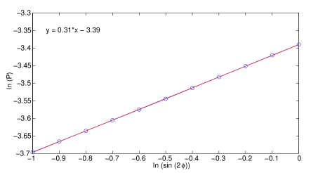
Figure 2: Logarithmic plot of $P$ versus $\sin(2\phi)$ for $q=2$ and $\tau=8$. The linear fit to the points has a slope of $0.31$.

For $q=3$, our arguments show that $P$ should scale as $(\cos(3\phi))^{1/4}/\tau^{3/4}$. Fig. 3 shows a logarithmic plot of $P$ versus $\tau$ for $\phi=0$; a linear fit gives a slope of $-0.77$ which is in good agreement with the expected value of $-3/4$. Figure 4 shows a plot of $p_{k}$ versus $(k+5\pi/6)\tau^{3/4}$ for three values of $\tau$, for $\phi=0$; the three curves are seen to coincide, indicating that $p_{k}$ is indeed a function of the scaling variable $(k+5\pi/6)\tau^{3/4}$ as indicated in Eq. (28), and only a range of values of $k+5\pi/6$ of the order of $1/\tau^{3/4}$ is seen to contribute significantly to the total excitation probability.

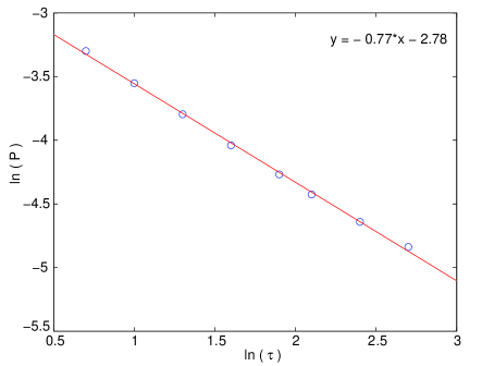
Figure 3: Logarithmic plot of $P$ versus $\tau$ for $q=3$ and $\phi=0$. The linear fit to the points has a slope of $-0.77$.

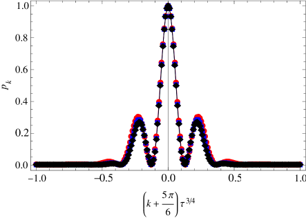
Figure 4: Plot of $p_{k}$ versus $(k+5\pi/6)\tau^{3/4}$ for $\tau=2$ (red), 4 (blue) and 8 (black), for $q=3$ and $\phi=0$.

Figure 4 shows several oscillations in $p_{k}$ as a function of $k$. To obtain a clearer understanding of these oscillations, we study in the Appendix a two-level system in which the one of the terms in the Hamiltonians varies in time as $|t|^{q}sgn(t)$; this is motivated by the form of the Hamiltonian in Eq. (28). We find that the number of oscillations increases with $q$. Our analysis also provides a derivation of the period of oscillation for large $q$, indicating that the oscillations in $k$ have a period that also scales as $1/\tau^{q/(q+1)}$; this follows from the statement proved in the Appendix that, for large values of $q$, the oscillations have a period $\pi/2$ in a parameter $b$ which is equal to the quantity $4k^{\prime}(\tau^{q}/f(q\phi))^{1/(q+1)}$ in Eq. (28). To see the manner in which $p_{k}$ depends on $q$, we have plotted $p_{k}$ versus $k+21\pi/22$ for $q=11$ and $\phi=0$ in Fig. 5. Note that for $q=11$, $p_{k}$ is expected to be a function of $(k+21\pi/22)\tau^{11/12}$; the figure indicates that only a range of values of $k+21\pi/22$ of the order of $1/\tau^{11/12}$ contributes substantially to the excitation probability. The number of oscillations in $p_{k}$ shows a clear increase compared to the case of $q=3$ in Fig. 4.

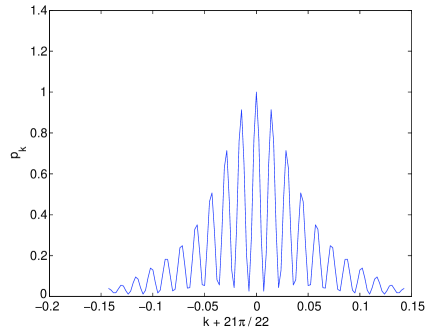
Figure 5: Plot of $p_{k}$ versus $k+21\pi/22$ for $q=11$, $\phi=0$, and $\tau=16$.

Our numerical simulations thus confirm the scaling behavior of $P$ as a function of the quenching rate and off-set $\phi$, showing that the scaling holds for a significant range of parameter space. They also illustrate the exact manner in which $p_{k}$ varies as a function of momentum $k$ and periodicity $q$.

IV More complex periodic structures

In the previous sections, we have considered a magnetic field given by $h_{n}=h\cos(\pi n/q+\phi)$ assuming even periodicity $2q$, and we have varied $h$ in time as $t/\tau$. Our analysis of the energy spectrum close to the points $k=\pm\pi/2$ and the scaling of the excitation probability were based on perturbation theory. We can now ask if other periodic forms for $h_{n}$ lead to similar results.

We again assume that $h_{n}=h\cos(Qn+\phi)$, but we set $Q=\pi p/q$, where $Q<2\pi$, $p$ and $q$ are relatively prime integers, and $p$ is odd. These conditions ensure that the period of $h_{n}$ is an even integer given by $2q$, so that the ground states for $h$ very large and either positive or negative are both half-filled. Once again we can do perturbation theory to obtain the matrix element between the states at $k=\pm\pi/2$; we find that at the lowest order in $h$ which is given by $h^{q}$, the magnitude of the matrix element is given by Eq. (11) regardless of the value of $p$. This follows from the number theoretic fact that the sets of integers $(1,2,\cdots,q-1)$ and $(p,2p,\cdots,p(q-1))$ modulo $q$ are identical if $p$ and $q$ are relatively prime niven ; thus the set of positive numbers $|\sin(\pi sp/q)|$, for $s=1,2,\cdots,q-1$, is the same for all values of $p$ which are relatively prime to $q$. Hence the effective two-level problem given in Eq. (19) depends only on $q$ and not on $p$.

As a simple example, we compare the cases given by $Q=\pi/4$ and $Q=3\pi/4$. For both of these, $h_{n}$ has period 8, and for small $h$, perturbation theory leads to the same expression for the magnitude of the matrix element given in Eq. (11) between the states at $k=\pm\pi/2$, namely, $|\Delta|=(1/16)h^{4}|\sin(4\phi)|$; we therefore obtain the same effective two-level problem given in Eq. (19). However, the complete 8-dimensional Hamiltonians $H_{k}$ are not identical for $Q=\pi/4$ and $3\pi/4$ for arbitrary values of $h$ and $k$, even if we allow for unitary transformations. It is therefore interesting to compare the results for the excitation probabilities $p_{k}$ in these two cases. This is shown in Figs. 6 and 7; we see that the forms of $p_{k}$ are qualitatively very similar although they differ quantitatively in the two cases.

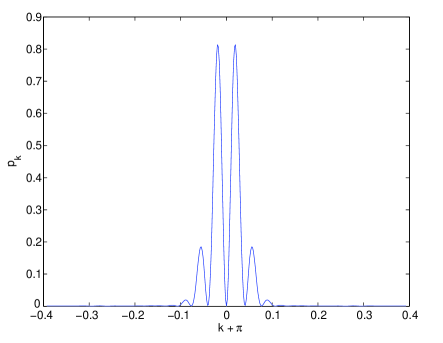
Figure 6: Plot of $p_{k}$ versus $k+\pi$ for $Q=\pi/4$, $\phi=\pi/8$, and $\tau=8$.

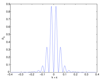
Figure 7: Plot of $p_{k}$ versus $k+\pi$ for $Q=3\pi/4$, $\phi=\pi/8$, and $\tau=8$.

Next, we consider the situation in which the magnetic field $h_{n}$ is periodic in $n$, but has several Fourier components. (We continue to assume that the period of $h_{n}$ is even, with $h_{n}$ being positive on half the sites and negative on the other half). For instance, let us consider a field of the form $h_{n}=h[a_{1}\cos(\pi n)+a_{2}\cos(\pi n/2+\pi/4)]$, where $a_{1}$, $a_{2}$ and $\phi$ are constants; we then vary $h$ as $t/\tau$. (In order to to focus on the scaling with respect to the quenching rate, we have chosen the phase of the period 4 term to be $\pi/4$ such that $\sin(2\phi)=1$). If the $a_{i}$’s are small, the perturbation theory described in Sec. II shows that there is a coupling between the low-energy states at $k=\pm\pi/2$ at first order in $a_{1}$ and at second order in $a_{2}$; these would lead to a total excitation probability scaling as $a_{1}^{1/2}/\tau^{1/2}$ and $(a_{2})^{2/3}/\tau^{2/3}$ respectively. Assuming that $a_{1}$ and $a_{2}$ are both non-zero, we expect that for very large values of $\tau$, the $1/\tau^{1/2}$ scaling would dominate over the $1/\tau^{2/3}$ scaling. But if $\tau$ is not too large, then the $1/\tau^{2/3}$ scaling could dominate if the values of $\tau$, $a_{1}$ and $a_{2}$ are such that $(a_{2})^{2/3}/\tau^{2/3}\gg a_{1}^{1/2}/\tau^{1/2}$. In particular, if $(a_{2})^{2/3}\gg a_{1}^{1/2}$, we may expect to see a $1/\tau^{2/3}$ scaling over a range of values of $\tau$ before crossing over to a $1/\tau^{1/2}$ scaling for very large values of $\tau$. Figure 8 shows a logarithmic plot of $P$ versus $\tau$ for the case $h_{n}=(t/\tau)[0.2\cos(\pi n)+\cos(\pi n/2+\pi/4)]$ (corresponding to $a_{1}=0.2$ and $a_{2}=1$), along with two linear fits near the beginning and end of the plot. The linear fits have slopes of $-0.65$ and $-0.48$ which are in good agreement with the values $-2/3$ and $-1/2$ respectively.

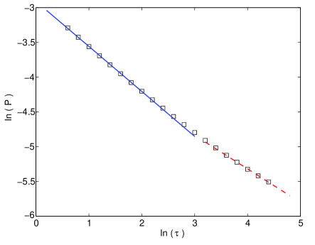
Figure 8: Logarithmic plot of $P$ versus $\tau$ for $h_{n}=(t/\tau)[0.2\cos(\pi n)+\cos(\pi n/2+\pi/4)]$ showing a cross-over between two power laws. The two linear fits near the beginning and end of the plot have slopes of $-0.65$ (blue solid) and $-0.48$ (red dashed) respectively.

Finally, we may ask what happens if $Q=\pi p/q$, where $q$ is very large and the variation of the potential is very slow. (For instance, this would be useful if we were interested in studying the case of a quasiperiodic pattern of the field $h_{n}$, and we approached such a pattern by taking rational approximations of the form $p/q$ with $q$ becoming progressively large). Unfortunately, it seems to be rather difficult to study the case of very large $q$ either analytically or numerically. Perturbation theory up to $q$-th order in $h$ would not be reliable, since the energies appearing in the denominator of Eq. (10), $\sin(\pi s/q)$, come arbitrarily close to zero if $s$ is held fixed and $q\to\infty$. Numerical calculations based on time evolution with the $2q$-dimensional Hamiltonian $H_{k}$ in Eq. (7), with $h=t/\tau$, also become difficult if $q$ is very large since there would be a large number of levels which come close to each other at different times; the time evolution would therefore need to be done very accurately to go from $t=-\infty$ to $t=\infty$. In this limit, further studies and alternate methods are called for.

V Quenching in a Tomonaga-Luttinger liquid

We have studied quenching in a periodic system of free fermions; we now turn to the manner in which this physics becomes modified in the presence of interactions between fermions. Our arguments borrow from the quenching treatment of Ref. degrandi, for interacting bosons in a periodic potential favoring one particle per potential minimum, adapting it to the situation of interacting fermions as well as generalizing to multiple boson occupancy.

Tracing back to our initial starting point, the spin Hamiltonian of Eq. (1), the addition of a nearest-neighbor $zz$ coupling of the form $J_{z}\sigma_{n}^{z}\sigma_{n+1}^{z}$ results in an interaction term in the fermionic system. Employing the Jordan-Wigner transformation described in Sec. II leads to the addition of a four-fermion interaction of the form $c_{n}^{\dagger}c_{n}c_{n+1}^{\dagger}c_{n+1}$ in the transformed fermionic Hamiltonian of Eq. (3).

We can treat the effect of these interactions on the quenching process described in the previous sections as follows. The quenching involves tuning the strength of the periodic potential $h$ from $-\infty$ to $+\infty$ as a function of time, and once again, the most important contribution to quenching dynamics comes from the gapless region at vanishing $h$. We can thus consider the low-energy physics of the fermionic system for small $h$, namely the effective Hamiltonian Eq. (12) which consists of right-moving and left-moving linear modes at Fermi points $k=\pm\pi/2$, $\psi_{R}$ and $\psi_{L}$, respectively, and a coupling between them of order $h^{q}$ derived from $q$-th order perturbation. In addition, we now have interactions and these can be treated within the standard context of bosonization, where the right and left moving modes $\psi_{R/L}\sim\exp[i\sqrt{\pi}~{}(\mp\sqrt{K}\Phi+\theta/\sqrt{K})]$ are expressed in terms of the bosonic fields $\Phi$ and $\theta$ gogolin . In terms of the scalar field $\Phi$, the deviation of the density of fermions $\rho$ from the average density $\rho_{0}$ is given by $\rho-\rho_{0}=-(\sqrt{K/\pi})\partial\Phi/\partial x$. The Luttinger parameter $K$ characterizes the strength of the interactions ($K<(>)1$ for repulsive (attractive) interactions, $K=1$ in the absence of interactions.) For a mapping from the spin model, the procedure can be considered in the range $-1<J_{z}\leq 1$; the parameter $K$ is then given by $K=\frac{\pi}{2\cos^{-1}(-J_{z})}$, so that $K$ goes from $\infty$ to $1/2$ as $J_{z}$ goes from $-1$ to 1.

The linear modes at $k=\pm\pi/2$ and the short-range fermion interactions together provide the standard action describing a Tomonaga-Luttinger liquid (TLL):

$$S~{}=~{}\frac{1}{2}~{}\int\int dtdx~{}\left[~{}\left(\frac{\partial\Phi}{\partial t}\right)^{2}~{}-~{}\left(\frac{\partial\Phi}{\partial x}\right)^{2}\right].$$ (31)

(Here, the velocity of the bosonic excitations has been set to unity.) The contribution of the $quench$ term to the action has the sine-Gordon form

$$S_{m}~{}\sim~{}\int\int dtdx~{}h^{q}~{}\cos(2\sqrt{\pi K}\Phi),$$ (32)

Compared to the standard cases of interacting fermions that result in forms similar to Eq. (31) and (32), we emphasize that these terms have been derived as the low-energy description of a system having a higher periodicity $2q$, resulting in the key dependence of the mass term $S_{m}$ on $q$.

Using Eqs. (31) and (32) as the starting point, we invoke renormalization group (RG) arguments gogolin to derive the scaling of defect formation due to the quench. By computing the correlation function of the operator $\cos(2\sqrt{\pi K}\Phi)$ at two different space-time points, one can show that it has mass dimension $K$; let us denote the coefficient of this operator in the action by $\mu$ in general. The parameter $\mu$ effectively becomes dependent on the length scale $L$, satisfying the RG equation $d\mu/d\ln L=(2-K)\mu$. Given the initial value of $\mu(a)=h^{q}$ at some microscopic length scale $a$ (this could be either the lattice spacing or the average distance between the particles in a continuum model), the solution of the RG equation is $\mu(L)=h^{q}(L/a)^{2-K}$. Assuming that $h^{q}\ll 1$, we see that $\mu(L)$ is of order 1 at a length scale given by $L=\xi$, where $(\xi/a)\sim 1/h^{q/(2-K)}$. The condition that $\mu(\xi)\sim 1$ implies that we have reached a strong coupling (disordered) regime at the length scale $\xi$, i.e., $\xi$ is the correlation length of the theory. Since $h$ denotes the deviation from the quantum critical point, the relation $\xi/a\sim 1/h^{q/(2-K)}$ implies that the correlation length exponent is given by $\nu=q/(2-K)$. As argued in the previous sections, if $h$ is quenched through the QCP at $h=0$ at a rate given by $1/\tau$, the KZ scaling form then implies that the density of defects will scale as $1/\tau^{d\nu/(z\nu+1)}$. Hence, substituting the value of $\nu$ in this scaling form, the density of defects scales as

$$\rho_{D}\sim 1/\tau^{q/(q+2-K)}.$$ (33)

This scaling behavior can be derived more rigorously by trivially modifying the treatment in Ref. degrandi, to include the $q$ dependence. For the non-interacting case, $K=1$, this form reproduces the earlier expression $1/\tau^{q/(q+1)}$. In the presence of interactions, we see that the power varies continuously with $K$. We note that the power law $1/\tau^{q/(q+2-K)}$ is only valid for $1/2<K<2$. The value $K=2$ corresponds to a Kosterlitz-Thouless transition. For $K>2$, the cosine term in the action is irrelevant. It has been argued in Ref. degrandi, that the probability of excitations then receives contributions from all modes, not just the low-energy modes near $k=\pm\pi/2$; hence the scaling law has the form $1/\tau$ regardless of the value of $q$.

These arguments can be used to generalize the results of Ref. degrandi, to a multi-boson situation. In addition to fermionic systems, the TLL form can be equally well applied to one-dimensional systems of repulsively interacting bosons; the Luttinger parameter $K$ goes from $\infty$ to $1$ as the strength of the repulsive interaction is varied from zero to $\infty$. In particular, when the interaction strength is infinitely large, the bosonic system is equivalent to a system of non-interacting spinless fermions lieb63 with $K=1$. In the continuum of interacting bosons described by the action in Eq. (31), one can introduce a spatially periodic potential of the form $V(x,t)=h(t)\cos(2\pi\rho x/q)$, where $q$ is an integer. For very large values of $h(t)$, the ground state would have exactly $q$ particles residing in each of the minima of this potential. (Therein lies the generalization of Ref. degrandi, which assumes $q=1$.) To analyze a quench of the form $h=t/\tau$, we note that there is a one-to-one correspondence between the interacting system of bosons and that of the fermions studied above. Focusing on the lower energy physics, once again Eq. (31) describes a gapless TLL with a Fermi momentum given by $k_{F}=\pi\rho$ while Eq. (32) describes the contribution coming from a small, non-vanishing $h$. The subsequent analysis above also goes through for the bosonic case except for a redefinition of the interaction parameter. We thus conclude that the density of defects (which corresponds to some of the potential wells having either more than or less than $q$ particles) scales as $1/\tau^{q/(q+2-K)}$ as in Eq. (32) if $K<2$, and as $1/\tau$ if $K>2$.

VI Conclusion

To summarize, we have studied the dynamics of a spin-1/2 chain in which the amplitude of a spatially periodic magnetic field $h\cos(Qn+\phi)$ is slowly varied in time so as to take the system across a quantum critical point. We have equivalently analyzed a system of spinless fermions with a spatially periodic and time-dependent chemical potential. We find that a quenching rate of $1/\tau$ takes the system to a final state having a density of defects that scales as $1/\tau^{q/(q+1)}$ for $Q=\pi/q$; the power depends on the period of the magnetic field. We have shown this by using perturbation theory to derive an effective Hamiltonian for pairs of states near zero energy; this Hamiltonian has a parameter varying as a power of the time, where this power also depends on the period of the field. We have confirmed our results numerically in a number of cases. If the magnetic field has several Fourier components, the power law corresponding to the smallest period is found to dominate for very small values of $1/\tau$ although one may find a cross-over at intermediate values of $\tau$ depending on the amplitudes of the different Fourier components. If the spin Hamiltonian has additional terms which can be mapped to interactions between the fermions, the power varies continuously with the interaction strength. To obtain a better understanding of some features of the excitation probability in the spin chain problem, we have numerically studied a two-level system in which a term in the Hamiltonian varies as a power law in time. We find that the excitation probability in this problem has a complicated dependence on the power resembling the results obtained for the many-body spin or fermion systems.

Our predictions, of interest from the perspective of critical phenomena and out-of-equilibrium dynamics, can be investigated in various physical systems. The most immediate experimental realizations would perhaps be in the area of cold atoms or molecules trapped in effectively one-dimensional optical lattices coldatoms , where tuning parameters is easy and quenching has become an extensive topic of study. Another area would be one that has been studied in great depth and well characterized, namely, various physical systems described by spin chain physics. In this case, the only additional ingredient necessary would be to subject the chains to a magnetic field having a periodic modulation in space and whose strength could be dynamically tuned. As yet another instance, recent proposals have employed effectively spinless $p$-wave paired fermionic superconducting wires in schemes for topological quantum computation requiring tuning between topological and non-topological regions in these wires. As described in our previous workwade , periodic potentials in such systems offer a way of studying topological aspects. A systematic study of the quench work presented here generalized to include anomalous terms due to superconductivity (already initiated in Ref. wade, ) would be useful for the proposed schemes and as a study in of itself on quenches in topological systems.

Our results have revealed how mode coupling can retain the slow out-of-equilibrium dynamics expected of quenching through a QCP while giving it a richer, more complex structure. Here, the mode coupling was via fragmentation of the Brillouin zone by a periodic potential. Future avenues would involve more intricate mode coupling, for instance, in the presence of quasiperiodic potentials, or in disordered systems, which completely break translation invariance and can undergo delocalization-localization transitions, or even in systems of weakly coupled isolated quantum states. Finally, our studies have all been in the zero temperature limit. Since the quantum critical regime extends up to some finite range of temperatures, we expect the results presented here to persist at temperatures which are much smaller than the energy gap at the initial time patane ; a rigorous finite-temperature study is in order.

Appendix A Non-linear quenching in the Landau-Zener system

In this Appendix, we will study a generalization of the Landau-Zener problem lz ; majorana in which the Hamiltonian varies non-linearly in time. We consider a two-level system evolving with a time-dependent Hamiltonian as

$$i\frac{d}{dt}\left(\begin{array}[]{c}u_{1}\\ u_{2}\end{array}\right)=\left(\begin{array}[]{cc}|t|^{q}sgn(t)&b\\ b&-|t|^{q}sgn(t)\end{array}\right)\left(\begin{array}[]{c}u_{1}\\ u_{2}\end{array}\right),$$ (40)

(41)

where $b$ is a constant, and $q$ is a positive integer. It is sufficient to study this problem for the case that $b$ is real and positive, since the Hamiltonian for any complex value of $b$ is related by a unitary transformation to a Hamiltonian in which $b$ is replaced by $|b|$. The reason for studying the Hamiltonian in Eq. (41) is that it is related by a unitary transformation to the one in Eq. (28), with $b$ playing the role of $2k^{\prime}(\tau^{q}/f(q\phi))^{1/(q+1)}$. Note that we have taken the time dependence in (41) to be of the form $|t|^{q}sgn(t)$; this has been done so that the ground states for $t\to-\infty$ and $t\to\infty$ are given by $(u_{1},u_{2})=(1,0)$ and $(0,1)$ respectively, just as they are for the case of linear time variation ($q=1$).

Note that we have taken the time dependence in (41) to be of the form $|t|^{q}sgn(t)$, rather than $t^{q}$; the two expressions agree for $q$ odd, but not for $q$ even. We have chosen the form $|t|^{q}sgn(t)$ so that for all values of $q$, the ground states for $t\to-\infty$ and $t\to\infty$ are given by $(u_{1},u_{2})=(1,0)$ and $(0,1)$ respectively, just as they are for the case of linear time variation ($q=1$).

At $t=-\infty$, we begin with the ground state $(u_{1},u_{2})=(1,0)$. We then numerically evolve the wave function as in Eq. (41) up to $t=\infty$; at that point, we find the excitation probability given by $p(b)=|u_{1}(\infty)|^{2}$. For $b=0$, we expect $p=1$ since the Hamiltonian has no matrix element connecting the initial and final ground states; hence the system remains in the initial ground state (the sudden limit). For $b\to\infty$, we expect $p=0$ since the instantaneous ground and excited states remain well separated at all times; hence the system follows the instantaneous ground state (the adiabatic limit). For $q=1$, one has the exact expression $p(b)=\exp(-\pi b^{2})$ lz . For $q\geq 2$, the exact expression for $p(b)$ is not known.

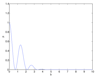
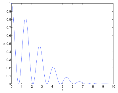
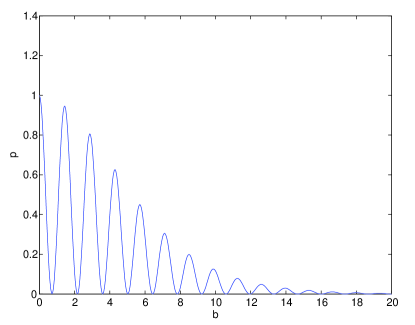
Figure 9: Plot of $p$ versus $b$ for $q=5$ (top), $q=10$ (middle), and $q=20$ (bottom).

Figure 9 shows how $p$ varies with $b$ for three different values of $q$. We see that $p(b)$ is a product of an oscillatory function and a decaying function of $b$ (this seems to be true for all values of $q\geq 2$). The period of oscillations appears to approach $\pi/2$ for large values of $q$ and small values of $b$. We can understand this as follows. If $q\gg 1$, the function $|t|^{q}$ is much larger than 1 for $|t|>1$ and much smaller than 1 for $|t|<1$. Let us therefore make the approximation $|t|^{q}=\infty$ for $|t|>1$ and $=0$ for $|t|<1$. The Hamiltonian in Eq. (41) can then be written as

$$H = \left(\begin{array}[]{cc}-\infty&b\\ b&\infty\end{array}\right)~{}~{}~{}{\rm for}~{}~{}~{}t~{}<~{}-1,$$ (44)

$$= \left(\begin{array}[]{cc}0&b\\ b&0\end{array}\right)~{}~{}~{}{\rm for}~{}~{}~{}-1~{}<~{}t~{}<~{}1,$$ (47)

$$= \left(\begin{array}[]{cc}\infty&b\\ b&-\infty\end{array}\right)~{}~{}~{}{\rm for}~{}~{}~{}1~{}<~{}t.$$ (50)

Since we begin with the wave function $(u_{1},u_{2})=(1,0)$ at $t=-\infty$, and the energy levels are given by $\pm\infty$ from $t=-\infty$ up to $t=1$, the wave function remains equal to $(1,0)$ (times a phase factor due to time evolution with infinite energy) up to $t=-1$. Then the Hamiltonian is independent of time from $t=-1$ to $t=1$; this is known as the waiting problem divakaran . It is easy to solve for the time evolution during this period; we find that the wave function at $t=1$ is given by $(\cos(2b),i\sin(2b))$ times a phase factor. From $t=-1$ to $t=\infty$, the energy levels are again given by $\pm\infty$; hence the wave function at $t=\infty$ is given by $u_{1}=\cos(2b)$ times a phase factor and $u_{2}=\sin(2b))$ times another phase factor. We thus obtain $p(b)=\cos^{2}(2b)$. This explains the oscillations in $p$ versus $b$ with period $\pi/2$ and amplitude equal to $1/2$ for large values of $q$ and small values of $b$. However, this simple explanation breaks down for large values of $b$ where the period of oscillations starts deviating from $\pi/2$ and the amplitude of oscillations goes to zero as we can see in Fig. 9.

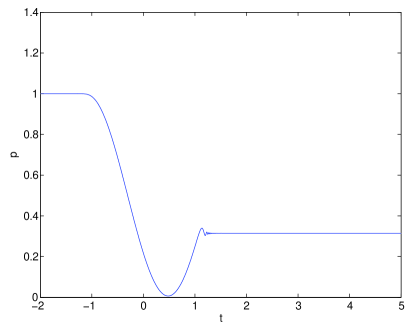
Figure 10: Plot of $p$ versus $t$ for $q=20$ and $b=1$.

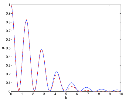
Figure 11: Two-parameter fit to plot of $p$ versus $b$ for $q=10$. The fitting function $p(b)=e^{-c_{1}b^{2}}\cos^{2}(2c_{2}b)$ gives $c_{1}=0.091$ and $c_{2}=1.11$.

Figure 10 confirms the scenario presented above for the variation of the excitation probability $p=|u_{1}|^{2}$ versus the time $t$. Namely, $p$ does not change much before $t=-1$ or after $t=1$, but it oscillates between $t=-1$ and $1$. Figure 11 shows a two-parameter fit to a plot of $p$ versus $b$ for $q=10$; a function of the form $p(b)=e^{-c_{1}b^{2}}\cos^{2}(2c_{2}b)$ with $c_{1}=0.091$ and $c_{2}=1.11$ gives a good fit for $b\lesssim 3.5$, but the fit becomes progressively worse for larger values of $b$. For $q=20$, we find that the same function of $p$ versus $b$ gives a good fit with $c_{1}=0.020$ and $c_{2}=1.08$ for $b\lesssim 5.5$. Note that our analysis above predicts that $c_{2}$ should be equal to 1.

The study of the two-level system in this Appendix sheds some light on the results we obtained in Sec. III for the spin system. In particular, the observation in Fig. 9 that as $q$ increases, $p(b)$ shows increased oscillation as a function of $b$ (while the amplitude of the oscillations goes to zero for large $b$) explains similar features seen in Figs. 4 and 5 for the spin system.

References

- (1)
- (2) T. W. B. Kibble, J. Phys. A 9, 1387 (1976), and Phys. Rep. 67, 183 (1980); W. H. Zurek, Nature (London) 317, 505 (1985), and Phys. Rep. 276, 177 (1996).
- (3) W. H. Zurek, U. Dorner, and P. Zoller, Phys. Rev. Lett. 95, 105701 (2005); J. Dziarmaga, Phys. Rev. Lett. 95, 245701 (2005); B. Damski, Phys. Rev. Lett. 95, 035701 (2005).
- (4) A. Polkovnikov, Phys. Rev. B 72, 161201(R) (2005); A. Polkovnikov and V. Gritsev, Nature Phys. 4, 477 (2008).
- (5) P. Calabrese and J. Cardy, J. Stat. Mech. P04010 (2005), and Phys. Rev. Lett. 96, 136801 (2006).
- (6) R. W. Cherng and L. S. Levitov, Phys. Rev. A 73, 043614 (2006).
- (7) V. Mukherjee, U. Divakaran, A. Dutta, and D. Sen, Phys. Rev. B 76, 174303 (2007); U. Divakaran, A. Dutta, and D. Sen, Phys. Rev. B 78, 144301 (2008); S. Deng, G. Ortiz, and L. Viola, EPL 84, 67008 (2008); U. Divakaran, V. Mukherjee, A. Dutta, and D. Sen, J. Stat. Mech: Theory Exp. P02007 (2009); V. Mukherjee and A. Dutta, EPL 92, 37004 (2010).
- (8) A. Dutta, R. R. P. Singh, and U. Divakaran, EPL 89, 67001 (2010); T. Hikichi, S. Suzuki, and K. Sengupta, Phys. Rev. B 82, 174305 (2010).
- (9) K. Sengupta, D. Sen, and S. Mondal, Phys. Rev. Lett. 100, 077204 (2008); S. Mondal, D. Sen, and K. Sengupta, Phys. Rev. B 78, 045101 (2008).
- (10) D. Sen, K. Sengupta, and S. Mondal, Phys. Rev. Lett. 101, 016806 (2008); S. Mondal, K. Sengupta, and D. Sen, Phys. Rev. B 79, 045128 (2009).
- (11) R. Barankov and A. Polkovnikov, Phys. Rev. Lett. 101, 076801 (2008); C. De Grandi, V. Gritsev, and A. Polkovnikov, Phys. Rev. B 81, 012303 (2010).
- (12) D. Patanè, A. Silva, L. Amico, R. Fazio, and G. E. Santoro, Phys. Rev. Lett. 101, 175701 (2008).
- (13) C. de Grandi, R. Barankov, and A. Polkovnikov, Phys. Rev. Lett. 101, 230402 (2008).
- (14) A. Bermudez, D. Patanè, L. Amico, and M. A. Martin-Delgado, Phys. Rev. Lett. 102, 135702 (2009).
- (15) D. Sen and S. Vishveshwara, EPL 91, 66009 (2010).
- (16) F. Pollmann, S. Mukerjee, A. M. Turner, and J. E. Moore, Phys. Rev. E 81, 020101(R) (2010).
- (17) J. Dziarmaga, Advances in Physics 59, 1063 (2010); A. Polkovnikov, K. Sengupta, A. Silva, and M. Vengalattore, Rev. Mod. Phys. 83, 863 (2011); A. Dutta, U. Divakaran, D. Sen, B. K Chakrabarti, T. F. Rosenbaum, and G. Aeppli, arXiv:1012.0653.
- (18) W. DeGottardi, D. Sen, and S. Vishveshwara, New J. Phys 13, (2011) 065208.
- (19) A. Kitaev, Ann. Phys. (N.Y.) 321, 2 (2006).
- (20) X.-Y. Feng, G.-M. Zhang, and T. Xiang, Phys. Rev. Lett. 98, 087204 (2007).
- (21) H.-D. Chen and Z. Nussinov, J. Phys. A 41, 075001 (2008); Z. Nussinov and G. Ortiz, Phys. Rev. B77, 064302 (2008); G. Baskaran, S. Mandal, and R. Shankar, Phys. Rev. Lett. 98, 247201 (2007); K. P. Schmidt, S. Dusuel, and J. Vidal, Phys. Rev. Lett. 100, 057208 (2008); D.-H. Lee, G.-M. Zhang, and T. Xiang, Phys. Rev. Lett. 99, 196805 (2007).
- (22) M. Z. Hasan and C. L. Kane, Rev. Mod. Phys. 82, 3045 (2010).
- (23) C. Zener, Proc. Roy. Soc. London, Ser. A 137, 696 (1932); L. Landau and E. M. Lifshitz, Quantum Mechanics: Non-relativistic Theory, 2nd Ed. (Pergamon Press, Oxford, 1965).
- (24) E. Lieb, T. Schultz, and D. Mattis, Ann. Phys. (NY) 16, 407 (1961).
- (25) M. Ya. Azbel, Zh. Eksp. Teor. Fiz. 46, 929 (1964) [Sov. Phys. JETP 19, 634 (1964); D. R. Hofstadter, Phys. Rev. B 14, 2239 (1976).
- (26) W. Y. Hsu and L. M. Falicov, Phys. Rev. B 13, 1595 (1976); G. M. Obermair and H.-J. Schellnhuber, Phys. Rev. B 23, 5185 (1981); H.-J. Schellnhuber, G. M. Obermair, and A. Rauh, Phys. Rev. B 23, 5191 (1981); S. Ostlund and R. Pandit, Phys. Rev. B 29, 1394 (1984); S. N. Sun and J. P. Ralston, Phys. Rev. B 44, 13603 (1991); P. B. Wiegmann and A. V. Zabrodin, Phys. Rev. Lett. 72, 1890 (1994).
- (27) D. Sen and S. Lal, Phys. Rev. B 61, 9001 (2000), and Europhys. Lett. 52, 337 (2000).
- (28) I. Niven, H. S. Zuckerman, and H. L. Montgomery, An Introduction to the Theory of Numbers (John Wiley, Singapore, 2000).
- (29) A. O. Gogolin, A. A. Nersesyan, and A. M. Tsvelik, Bosonization and Strongly Correlated Systems (Cambridge University Press, Cambridge, 1998); J. von Delft and H. Schoeller, Ann. Phys. (Leipzig) 7, 225 (1998); G. D. Mahan, Many-Particle Physics (Kluwer Academic/Plenum Publishers, New York, 2000); S. Rao and D. Sen, in Field theories in Condensed Matter Physics, edited by S. Rao (Hindustan Book Agency, New Delhi, 2001); T. Giamarchi, Quantum Physics in One Dimension (Oxford University Press, Oxford, 2004); G. F. Giuliani and G. Vignale, Quantum Theory of the Electron Liquid (Cambridge University Press, Cambridge, 2005).
- (30) E. H. Lieb and W. Liniger, Phys. Rev. 130, 1605 (1963).
- (31) L.-M. Duan, E. Demler, and M. D. Lukin, Phys. Rev. Lett. 91, 090402 (2003); A. Micheli, G. K. Brennen, and P. Zoller, Nature Phys. 2, 341 (2006).
- (32) E. Majorana, Nuovo Cimento 9, 43 (1932); E. C. G. Stueckelberg, Helv. Phys. Acta 5, 369 (1932).
- (33) U. Divakaran, A. Dutta, and D. Sen, Phys. Rev. B 81, 054306 (2010).