Theta vacuum and entanglement interaction
in the three-flavor Polyakov-loop extended Nambu-Jona-Lasinio model

Abstract

We investigate theta-vacuum effects on the QCD phase diagram for the realistic 2+1 flavor system, using the three-flavor Polyakov-extended Nambu-Jona-Lasinio (PNJL) model and the entanglement PNJL model as an extension of the PNJL model. The theta-vacuum effects make the chiral transition sharper. For large theta-vacuum angle the chiral transition becomes first order even if the quark number chemical potential is zero, when the entanglement coupling between the chiral condensate and the Polyakov loop is taken into account. We finally propose a way of circumventing the sign problem on lattice QCD with finite theta.

I Introduction

The existence of instanton solution in quantum chromodynamics (QCD) requires the QCD Lagrangian with the theta vacuum:

$${\cal L}_{QCD} = \bar{q}_{f}(\gamma_{\nu}D_{\nu}+m_{f})q_{f}+\frac{1}{4}F^{a}_{\mu\nu}F^{a}_{\mu\nu}$$ (1)

$$-i\theta\frac{g^{2}}{64\pi^{2}}\epsilon_{\mu\nu\sigma\rho}F^{a}_{\mu\nu}F^{a}_{\sigma\rho}$$

in Euclidean spacetime, where $F^{a}_{\mu\nu}$ is the field strength of gluon Theta76 . Theoretically the angle $\theta$ can take any arbitrary value between $-\pi$ and $\pi$. However, experiments indicate $|\theta|<3\times 10^{-10}$ Baker ; Ohta . The Lagrangian is invariant under the combination of the parity transformation and the transformation $\theta\to-\theta$, so that parity ($P$) and charge-parity symmetry ($CP$) become exact only at $\theta=0$ and $\pm\pi$; note that $\theta=-\pi$ is identical with $\theta=\pi$ because of the periodicity $2\pi$ in $\theta$. Why should $\theta$ be so small? This long-standing puzzle is called the strong $CP$ problem; see Ref. Vicari and references therein for the detail.

For $T$ higher than the QCD scale $\Lambda_{\mathrm{Q}CD}$, there is a possibility that $\theta$ is effectively varied to finite values depending on spacetime coordinates $(t,x)$, since sphalerons are so activated as to jump over the potential barrier between the different degenerate ground states MMS . If this happens, $P$ and $CP$ symmetries can be violated locally in high-energy heavy-ion collisions or the early Universe at $T\approx\Lambda_{\mathrm{Q}CD}$. Actually, it is argued in Refs. Metlitski and Zhitnitsky (2005); Kharzeev and Zhitnitsky (2007) that $\theta$ may be of order 1 at the epoch of the QCD phase transition in the early Universe, whereas it vanishes at the present epoch Peccei ; Dine ; Zhitnitsky ; Shifman ; Kim . This finite value of $\theta$ could be a new source of large $CP$ violation in the early Universe and may be a crucial missing element for solving the puzzle of baryogenesis.

In the early stage of heavy-ion collision, the magnetic field is formed, while the effective $\theta(t,x)$ deviates the total number of particles plus antiparticles with right-handed helicity from those with left-handed helicity. As a consequence of this fact, an electromagnetic current is generated along the magnetic field, since particles with right-handed helicity move opposite to antiparticles with right-handed helicity. This is the so-called chiral magnetic effect Kharzeev ; Kharzeev and Zhitnitsky (2007); FKW ; Fukushima et al. (2010). The chiral magnetic effect may explain the charge separations observed in the recent STAR results Abelev . The thermal system with nonzero $\theta$ is thus quite interesting.

For vacuum with no temperature ($T$) and no quark-number chemical potential ($\mu$), parity $P$ is preserved when $\theta=0$ VW , but is spontaneously broken when $\theta=\pi$ Dashen ; Witten (1980). The $P$ violation, called the Dashen mechanism, is essentially nonperturbative, but the first-principle lattice QCD (LQCD) is not applicable for the case of finite $\theta$ because of the sign problem. Temperature ($T$) and/or quark-number chemical potential ($\mu$) dependence of the mechanism has then been analyzed by effective models such as the chiral perturbation theory Vecchia and Veneziano (1980); Smilga ; Tytgat ; ALS ; Creutz ; Metlitski and Zhitnitsky (2005), the Nambu-Jona-Lasinio (NJL) model Fujihara et al. (2010); Boer and Boomsma (2008a); Boomsma and Boer (2008a); Chatteriee et al (2011) and the Polyakov-loop extended Nambu-Jona-Lasinio (PNJL) model Kouno et al (2011); Sakai et al (2011).

Using the two-flavor NJL model Nambu and Jona-Lasinio (1961a); Asakawa and Yazaki (1989); Kashiwa et al (2006), Fujihara, Inagaki and Kimura made a pioneering work on the $P$ violation at $\theta=\pi$ Fujihara et al. (2010) and Boer and Boomsma studied this issue extensively Boer and Boomsma (2008a); Boomsma and Boer (2008a). In the previous works Kouno et al (2011); Sakai et al (2011), we extended the formalism to the two-flavor PNJL and entanglement PNJL (EPNJL) models and investigated effects of the theta vacuum on the QCD phase diagram. Very recently similar analyses were made for the realistic case of 2+1 flavors by using the NJL model Chatteriee et al (2011). It is then highly expected that the finite-$\theta$ effect is investigated in the 2+1 flavor case by using the PNJL and EPNJL models that are more reliable than the NJL model.

If QCD with finite $\theta$ is analyzed directly with LQCD, one can get conclusive results on the theta vacuum. Here we consider a way of minimizing the sign problem in LQCD. For this purpose we transform the quark field $q$ to the new one $q^{\prime}$ by the following $SU_{\rm A}(3)\otimes U_{\rm A}(1)$ transformation,

$$q_{u}=e^{i\gamma_{5}{\theta\over{4}}}q_{u}^{\prime},~{}~{}~{}~{}~{}q_{d}=e^{i\gamma_{5}{\theta\over{4}}}q_{d}^{\prime},~{}~{}~{}~{}~{}q_{s}=q_{s}^{\prime}.$$ (2)

The QCD Lagrangian is then rewritten into

$${\cal L}_{QCD}=\sum_{l=u,d}\bar{q}_{l}^{\prime}{\cal M}_{l}(\theta)q_{l}^{\prime}+\bar{q}_{s}^{\prime}{\cal M}_{s}q_{s}^{\prime}+\frac{1}{4}F^{a}_{\mu\nu}F^{a}_{\mu\nu}$$ (3)

with the new quark field $q^{\prime}$, where

$${\cal M}_{l}(\theta) \equiv \gamma_{\nu}D_{\nu}+m_{l}\cos{(\theta/2)}+m_{l}i\gamma_{5}\sin{(\theta/2)},$$ (4)

$${\cal M}_{s} \equiv \gamma_{\nu}D_{\nu}+m_{s}.$$ (5)

Only the Dirac operator ${\cal M}_{l}(\theta)$ has $\theta$ dependence in (3). The determinant of ${\cal M}_{l}(\theta)$ satisfies

$${\rm det}{\cal M}_{l}(\theta)=\left({\rm det}{\cal M}_{l}(-\theta)\right)^{\ast}.$$ (6)

The sign problem is thus induced by the $\theta$-odd ($P$-odd) term, $m_{l}i\gamma_{5}\sin{(\theta/2)}$. The difficulty of the sign problem is expected to be minimized in the QCD Lagrangian of (3), since the $\theta$-odd term includes the light quark mass $m_{l}$ that is much smaller than $\Lambda_{\rm QCD}$ as a typical scale of QCD. This point is discussed in this paper.

In this paper, we analyze effects of the theta vacuum on the QCD phase diagram for the realistic case of 2+1 flavors by using the three-flavor PNJL Matsumoto (2010) and EPNJL models Sasaki et al. (2011). Particularly, the three-flavor phase diagram is investigated in the $\mu$-$T$ plane with some values of $\theta$. Through the analysis, we finally propose a way of circumventing the sign problem on LQCD calculations with finite $\theta$.

This paper is organized as follows. In Sec. II, we recapitulate the three-flavor PNJL and EPNJL models. In Sec. III, numerical results are shown. Section IV is devoted to summary.

II Formalism

The three-flavor PNJL Lagrangian with the $\theta$-dependent anomaly term is obtained in Euclidean spacetime by

$${\cal L}= {\bar{q}}(\gamma_{\nu}D_{\nu}+{\hat{m}_{0}}-\gamma_{4}{\hat{\mu}})q$$

$$-G_{\rm S}\sum_{a=0}^{8}[({\bar{q}}\lambda_{a}q)^{2}+({\bar{q}}i\gamma_{5}\lambda_{a}q)^{2}]$$

$$+G_{\rm D}\Bigl{[}e^{i\theta}\det_{ij}{\bar{q}}_{i}(1-\gamma_{5})q_{j}+e^{-i\theta}\det_{ij}{\bar{q}}_{i}(1+\gamma_{5})q_{j}\Bigr{]}$$

$$+{\cal U}(\Phi[A],\Phi^{*}[A],T),$$ (7)

where $D_{\nu}=\partial_{\nu}-i\delta_{\nu 4}A_{4}^{a}{\lambda_{a}/2}$ with the Gell-Mann matrices $\lambda_{a}$. The corresponding PNJL Lagrangian in Minkowski spacetime is shown in Refs. Kouno et al (2011); Sakai et al (2011). The three-flavor quark fields $q=(q_{u},q_{d},q_{s})$ have masses ${\hat{m}_{0}}={\rm diag}(m_{u},m_{d},m_{s})$, and the chemical potential matrix ${\hat{\mu}}$ is defined by ${\hat{\mu}}={\rm diag}(\mu,\mu,\mu)$ with the quark-number chemical potential $\mu$. Parameters $G_{\rm S}$ and $G_{\rm D}$ denote coupling constants of the scalar-type four-quark and the Kobayashi-Maskawa-’t Hooft (KMT) determinant interaction Kobayashi and Maskawa (1970); ’t Hooft (1976), respectively, where the determinant runs in the flavor space. The KMT determinant interaction breaks the $U_{\mathrm{A}}(1)$ symmetry explicitly. Obviously, the theta-vacuum parameter $\theta$ has a periodicity of $2\pi$. We then restrict $\theta$ in a period $0\leq\theta\leq 2\pi$.

The gauge field $A_{\mu}$ is treated as a homogeneous and static background field in the PNJL model Meisinger et al. (1996); Fukushima (2004); Ratti et al. (2006); Rossner et al. (2007); Schaefer (2007); Kashiwa et al (2008); Sakai et al (2008, 2008); Kahara (2009); Kasihwa et al (2009); Kouno et al (2009); Matsumoto (2010); Sasaki et al. (2009, 2010); Sakai (2010); Gatto (2011); Kouno et al (2011); Sasaki et al. (2011); Sakai et al (2011). The Polyakov-loop $\Phi$ and its conjugate $\Phi^{*}$ are determined in the Euclidean space by

$$\Phi ={1\over{3}}{\rm tr}_{\rm c}(L),~{}~{}~{}~{}~{}\Phi^{*}={1\over{3}}{\rm tr}_{\rm c}({\bar{L}}),$$ (8)

where $L=\exp(iA_{4}/T)$ with $A_{4}/T={\rm diag}(\phi_{r},\phi_{g},\phi_{b})$ in the Polyakov-gauge; note that $\lambda_{a}$ is traceless and hence $\phi_{r}+\phi_{g}+\phi_{b}=0$. Therefore we obtain

$$\Phi = {1\over{3}}(e^{i\phi_{r}}+e^{i\phi_{g}}+e^{i\phi_{b}})$$

$$= {1\over{3}}(e^{i\phi_{r}}+e^{i\phi_{g}}+e^{-i(\phi_{r}+\phi_{g})}),$$

$$\Phi^{*} = {1\over{3}}(e^{-i\phi_{r}}+e^{-i\phi_{g}}+e^{-i\phi_{b}})$$ (9)

$$= {1\over{3}}(e^{-i\phi_{r}}+e^{-i\phi_{g}}+e^{i(\phi_{r}+\phi_{g})}).$$

We use the Polyakov potential $\mathcal{U}$ of Ref. Rossner et al. (2007):

$${\cal U}=T^{4}\Bigl{[}-\frac{a(T)}{2}{\Phi}^{*}\Phi$$

$$~{}~{}~{}~{}~{}+b(T)\ln(1-6{\Phi\Phi^{*}}+4(\Phi^{3}+{\Phi^{*}}^{3})-3(\Phi\Phi^{*})^{2})\Bigr{]}$$ (10)

with

$$a(T)=a_{0}+a_{1}\Bigl{(}\frac{T_{0}}{T}\Bigr{)}+a_{2}\Bigl{(}\frac{T_{0}}{T}\Bigr{)}^{2},~{}~{}~{}~{}b(T)=b_{3}\Bigl{(}\frac{T_{0}}{T}\Bigr{)}^{3}.$$ (11)

The parameter set in $\mathcal{U}$ is fitted to LQCD data at finite $T$ in the pure gauge limit. The parameters except $T_{0}$ are summarized in Table 1. The Polyakov potential yields a first-order deconfinement phase transition at $T=T_{0}$ in the pure gauge theory. The original value of $T_{0}$ is $270$ MeV determined from the pure gauge LQCD data, but the PNJL model with this value of $T_{0}$ yields a larger value of the pseudocritical temperature $T_{\mathrm{c}}$ of the deconfinement transition at zero chemical potential than $T_{\rm c}\approx 160$ MeV predicted by full LQCD Borsanyi etal (2010); Soeldner (2010); Kanaya (2010). Therefore we rescale $T_{0}$ to 195 (150) MeV so that the PNJL (EPNJL) model can reproduce $T_{\rm c}=160$ MeV Sasaki et al. (2011).

$a_{0}$	$a_{1}$	$a_{2}$	$b_{3}$
$3.51$	$-2.47$	$15.2$	$-1.75$

Table 1: Summary of the parameter set in the Polyakov-potential sector determined in Ref. Rossner et al. (2007). All parameters are dimensionless.

Now the quark field $q$ is transformed into the new one $q^{\prime}$ by (2) in order to remove $\theta$ dependence of the determinant interaction. As shown later, this transformation provides the thermodynamic potential $\Omega$ with a compact form and furthermore convenient to discuss the sign problem in LQCD. The present three-flavor PNJL model has 18 scalar and pseudoscalar condensates of quark-antiquark pair, but flavor off-diagonal condensates vanish for the system with flavor symmetric chemical potentials only Boer and Boomsma (2008a); Boomsma and Boer (2008a); Kouno et al (2011); Sakai et al (2011). Since the quark-number chemical potential considered in this paper is flavor diagonal, we can concentrate our discussion on flavor-diagonal condensates. Under the transformation (2), the flavor-diagonal quark-antiquark condensates, $\sigma_{f}=\bar{q}_{f}q_{f}$ and $\eta_{f}=\bar{q}_{f}i\gamma_{5}q_{f}$, are transformed into $\sigma_{f}^{\prime}=\bar{q}_{f}^{\prime}q_{f}^{\prime}$ and $\eta_{f}^{\prime}=\bar{q}_{f}^{\prime}i\gamma_{5}q_{f}^{\prime}$ as

$$\sigma_{l} = \cos{\left(\tfrac{\theta}{2}\right)}\sigma_{l}^{\prime}+\sin{\left(\tfrac{\theta}{2}\right)}\eta_{l}^{\prime},$$ (12)

$$\eta_{l} = -\sin{\left(\tfrac{\theta}{2}\right)}\sigma_{l}^{\prime}+\cos{\left(\tfrac{\theta}{2}\right)}\eta_{l}^{\prime},$$ (13)

$$\sigma_{s} = \sigma_{s}^{\prime},$$ (14)

$$\eta_{s} = \eta_{s}^{\prime}$$ (15)

for $l=u,d$. The Lagrangian is then rewritten into

$${\cal L}= {\bar{q}}^{\prime}(\gamma_{\nu}D_{\nu}+{\hat{m}_{0+}}+i{\hat{m}_{0-}}\gamma_{5}-\gamma_{4}{\hat{\mu}})q^{\prime}$$

$$-G_{\rm S}\sum_{a=0}^{8}[({\bar{q}}^{\prime}\lambda_{a}q^{\prime})^{2}+({\bar{q}}^{\prime}i\gamma_{5}\lambda_{a}q^{\prime})^{2}]$$

$$+G_{\rm D}\Bigl{[}\det_{ij}{\bar{q}}_{i}^{\prime}(1-\gamma_{5})q_{j}^{\prime}+\det_{ij}{\bar{q}}_{i}^{\prime}(1+\gamma_{5})q_{j}^{\prime}\Bigr{]}$$

$$+{\cal U}(\Phi[A],\Phi^{*}[A],T)$$ (16)

with

$$\hat{m}_{0+} = {\rm diag}(m_{u+},m_{d+},m_{s+})$$ (17)

$$= {\rm diag}\left(\cos{\left(\tfrac{\theta}{2}\right)}m_{u},~{}\cos{\left(\tfrac{\theta}{2}\right)}m_{d},~{}m_{s}\right),$$

$$\hat{m}_{0-} = {\rm diag}(m_{u-},m_{d-},m_{s-})$$ (18)

$$= {\rm diag}\left(\sin{\left(\tfrac{\theta}{2}\right)}m_{u},~{}\sin{\left(\tfrac{\theta}{2}\right)}m_{d},~{}0\right).$$

Making the mean-field approximation, one can obtain the mean-field Lagrangian as

$${\cal L}_{\rm MF} = {\bar{q}}^{\prime}(\gamma_{\nu}D_{\nu}+M_{f}^{\prime}+i\gamma_{5}N_{f}^{\prime}-\gamma_{4}{\hat{\mu}})q^{\prime}$$ (19)

$$+U_{M}+{\cal U}(\Phi[A],\Phi^{*}[A],T),$$

where

$$M_{f}^{\prime} = m_{f+}-4G_{\rm S}\sigma_{f}^{\prime}+2G_{\rm D}(\sigma^{\prime}_{f^{\prime}}\sigma^{\prime}_{f^{\prime\prime}}-\eta^{\prime}_{f^{\prime}}\eta^{\prime}_{f^{\prime\prime}}),$$ (20)

$$N_{f}^{\prime} = m_{f-}-4G_{\rm S}\eta_{f}^{\prime}-2G_{\rm D}(\sigma^{\prime}_{f^{\prime}}\eta^{\prime}_{f^{\prime\prime}}+\eta^{\prime}_{f^{\prime}}\sigma^{\prime}_{f^{\prime\prime}})$$ (21)

for $f\neq f^{\prime},~{}f\neq f^{\prime\prime},~{}f^{\prime}\neq f^{\prime\prime}$ and

$$U_{M} = 2G_{\rm S}\sum_{f=u,d,s}({\sigma_{f}^{\prime}}^{2}+{\eta_{f}^{\prime}}^{2})-4G_{\rm D}\sigma_{u}^{\prime}\sigma_{d}^{\prime}\sigma_{s}^{\prime}$$ (22)

$$+4G_{\rm D}(\sigma_{u}^{\prime}\eta_{d}^{\prime}\eta_{s}^{\prime}+\eta_{u}^{\prime}\sigma_{d}^{\prime}\eta_{s}^{\prime}+\eta_{u}^{\prime}\eta_{d}^{\prime}\sigma_{s}^{\prime}).$$

Performing the path integral over the quark field, one can obtain the thermodynamic potential $\Omega$ (per volume) for finite $T$ and $\mu$:

$$\Omega =-2\sum_{f=u,d,s}\int\frac{d^{3}{\bf p}}{(2\pi)^{3}}\Bigl{[}N_{\mathrm{c}}E_{f}$$

$$+\frac{1}{\beta}\ln~{}[1+3\Phi e^{-\beta(E_{f}-\mu)}+3\Phi^{*}e^{-2\beta(E_{f}-\mu)}+e^{-3\beta(E_{f}-\mu)}]$$

$$+\frac{1}{\beta}\ln~{}[1+3\Phi^{*}e^{-\beta(E_{f}+\mu)}+3\Phi e^{-2\beta(E_{f}+\mu)}+e^{-3\beta(E_{f}+\mu)}]\Bigl{]}$$

$$+U_{M}+{\cal U}(\Phi,\Phi^{*},T)$$ (23)

with $E_{f}=\sqrt{{\bf p}^{2}+{M_{f}^{\prime}}^{2}+{N_{f}^{\prime}}^{2}}$.

The three-dimensional cutoff for the momentum integration is introduced Matsumoto (2010), since this model is nonrenormalizable. For simplicity we assume the isospin symmetry for the ${u}$-${d}$ sector: $m_{l}\equiv m_{u}=m_{d}$. This three-flavor PNJL model has five parameters $G_{\rm S}$, $G_{\rm D}$, $m_{l}$, $m_{s}$ and $\Lambda$. One of the typical parameter sets is shown in Table 2. These parameters are fitted to empirical values of pion decay constant and $\pi$, $K$, $\eta^{\prime}$ meson masses at vacuum.

$m_{l}(\rm MeV)$	$m_{s}(\rm MeV)$	$\Lambda(\rm MeV)$	$G_{\rm S}\Lambda^{2}$	$G_{\rm D}\Lambda^{5}$
$5.5$	$140.7$	$602.3$	$1.835$	$12.36$

Table 2: Summary of the parameter set in the NJL sector taken from Ref. Rehnberg .

For imaginary $\mu$, $\Omega$ is invariant under the extended ${\mathbb{Z}}_{3}$ transformation Sakai et al (2008),

$$e^{\pm\mu/T}\to e^{\pm\mu/T}e^{\pm i{2\pi k\over{3}}},\quad\Phi\to\Phi e^{-i{2\pi k\over{3}}},$$

$$\Phi^{*}\to\Phi^{*}e^{i{2\pi k\over{3}}},$$ (24)

with integer $k$. This invariance ensures the Roberge-Weiss periodicity Roberge and Weiss (1986) in the imaginary chemical potential region Sakai et al (2008). Any reliable model should have this extended ${\mathbb{Z}}_{3}$ symmetry, when imaginary $\mu$ is taken in the model. This is a good test for checking the reliability of the model. The PNJL model has the extended ${\mathbb{Z}}_{3}$ symmetry Sakai et al (2008); Matsumoto (2010).

The four-quark vertex $G_{\rm S}$ is originated in a one-gluon exchange between quarks and its higher-order diagrams. If the gluon field $A_{\nu}$ has a vacuum expectation value $\langle A_{0}\rangle$ in its time component, $A_{\nu}$ is coupled to $\langle A_{0}\rangle$ and then to $\Phi$ through $L$. Hence we can modify $G_{\rm S}$ into an effective vertex $G_{\rm S}(\Phi)$ depending on $\Phi$ Kondo (2010). The effective vertex $G_{\rm S}(\Phi)$ is called the entanglement vertex and the model with this vertex is the EPNJL model. It is expected that $\Phi$ dependence of $G_{\rm S}(\Phi)$ will be determined in future by the accurate method such as the exact renormalization group method Braun (2010); Kondo (2010); Wetterich (1993). In this paper, however, we simply assume the following form for $G_{\rm S}(\Phi)$:

$$G_{\rm S}(\Phi)=G_{\rm S}[1-\alpha_{1}\Phi\Phi^{*}-\alpha_{2}(\Phi^{3}+\Phi^{*3})].$$ (25)

This form preserves the chiral symmetry, the charge conjugation ($C$) symmetry Kouno et al (2009) and the extended $\mathbb{Z}_{3}$ symmetry Sakai et al (2008). This entanglement vertex modifies the mesonic potential $U_{M}$, the dynamical quark masses $M_{f}^{\prime}$ and $N_{f}^{\prime}$. This is the three-flavor version of the EPNJL model. In principle, $G_{\rm D}$ can depend on $\Phi$, but $\Phi$ dependence of $G_{\rm D}$ is found to yield qualitatively the same effect on the phase diagram as that of $G_{\rm S}$. Following Ref. Sasaki et al. (2011), we neglect $\Phi$ dependence of $G_{\rm D}$ as a simple setup. In the present analysis, $\Phi$ dependence of $G_{\rm D}$ is thus renormalized in $\alpha_{1}$ and $\alpha_{2}$. The EPNJL model thus constructed keeps the extended ${\mathbb{Z}}_{3}$ symmetry.

The parameters $\alpha_{1}$ and $\alpha_{2}$ in (25) are fitted to two results of LQCD at finite $T$; one is the result of 2+1 flavor LQCD at $\mu=0$ YAoki that the chiral transition is crossover at the physical point and another is the result of degenerate three-flavor LQCD at $\mu=iT\pi$ FP2010 (2009) that the order of the RW phase transition at the RW endpoint is first order for small and large quark masses and second order for intermediate quark masses. The parameter set $(\alpha_{1},\alpha_{2})$ thus determined is located in the triangle region

$$\{-1.5\alpha_{1}+0.3<\alpha_{2}<-0.86\alpha_{1}+0.32,~{}\alpha_{2}>0\}.$$ (26)

In this paper we take $\alpha_{1}=0.25,~{}\alpha_{2}=0.1$ as a typical example, following Ref. Sasaki et al. (2011).

The classical variables $X=\Phi$, ${\Phi}^{*}$, $\sigma_{f}$ and $\eta_{f}$ are determined by the stationary conditions

$$\partial\Omega/\partial X=0.$$ (27)

The solutions to the stationary conditions do not give the global minimum of $\Omega$ necessarily. There is a possibility that they yield a local minimum or even a maximum. We then have checked that the solutions yield the global minimum when the solutions $X(T,\mu,\theta)$ are inserted into (23).

III Numerical results

In this section we show numerical results for the original condensates $(\sigma_{f},\eta_{f},\Phi)$, since this makes our discussion transparent. Under the parity transformation, $\sigma_{f}$, $\eta_{f}$ and $\Phi$ are transformed into $\sigma_{f}$, $-\eta_{f}$ and $\Phi$, respectively. This means that $\eta_{f}$ is $\theta$ odd while $\sigma_{f}$ and $\Phi$ are $\theta$ even, since the Lagrangian is invariant under the combination of the parity transformation and the transformation $\theta\to-\theta$. Thus $\eta_{f}$ is an order parameter of the spontaneous parity breaking, while $\sigma_{f}$ and $\Phi$ are approximate order parameters of the chiral and the deconfinement transitions, respectively. As an approximate order parameter of the chiral transition, $\sigma_{l}\equiv\sigma_{u}=\sigma_{d}$ is more proper than $\sigma_{s}$, since $m_{l}\ll m_{s}$.

III.1 Thermodynamics at $\mu=0$

In this subsection, we consider the case of $\mu=0$ where charge conjugation symmetry ($C$) is exact. Meanwhile, parity symmetry ($P$) is exact only at $\theta=0,~{}\pm\pi$, since $e^{i\theta}$ agrees with $e^{-i\theta}$ in (7) when $\theta=0,~{}\pm\pi$.

Figure 1 shows $T$ dependence of $\sigma_{l}$, $\sigma_{s}$ and $\Phi$ at $\theta=\mu=0$, where $\sigma_{l}$ and $\sigma_{s}$ are normalized by $\sigma_{0}=\sigma_{l}$ at $T=\mu=\theta=0$. Here $\sigma_{l}$ and $\Phi$ describe the chiral and deconfinement transitions, respectively. In the PNJL model of panel (a), the chiral restoration transition takes place after the deconfinement transition. In the EPNJL model of panel (b), meanwhile, both the transitions occur simultaneously. In the EPNJL model, $\sigma_{s}$ decreases rapidly near the pseudocritical temperature $T_{\rm c}=160$ MeV, but goes down gradually above $T_{\rm c}$. The rapid change of $\sigma_{s}$ comes from that of $\Phi$. For both the PNJL and EPNJL models, $\eta_{l}$ and $\eta_{s}$ are zero at any $T$. The $P$ symmetry is thus always preserved when $\theta=0$.

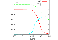
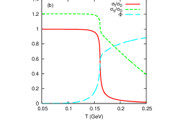
Fig. 1: $T$ dependence of the order parameters at $\theta=0$ and $\mu=0$ in (a) the PNJL model and (b) the EPNJL model. The solid, dashed and dotted lines represent $\sigma_{l}$, $\sigma_{s}$ and $\Phi$, respectively, where $\sigma_{l}$ and $\sigma_{s}$ are normalized by $\sigma_{0}=\sigma_{l}(T=\mu=\theta=0)$.

Figure 2 shows $\theta$ dependence of $\Omega$ and the order parameters at $T=\mu=0$ in the EPNJL model; note that the EPNJL model agrees with the PNJL model at $T=0$, since $G_{\rm S}(\Phi)=G_{\rm S}$ there because of $\Phi=0$. As shown in panel (a), $\Omega$ is $\theta$ even and has a cusp at $\theta=\pi$. This indicates that a first-order phase transition takes place at $T=\mu=0$ and $\theta=\pi$. As shown in panel (b), meanwhile, the $\eta_{f}$ are $\theta$ odd, while $\sigma_{f}$ and $\Phi$ are $\theta$ even. The condensate $\eta_{l}$ and $\eta_{s}$ have jumps at $\theta=\pi$, indicating that the first-order transition mentioned above is the spontaneous parity breaking. This is nothing but the Dashen phenomena Dashen .

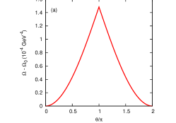
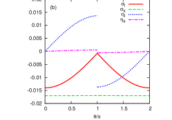
Fig. 2: $\theta$ dependence of (a) $\Omega$ and (b) the order parameters at $T=\mu=0$ in the EPNJL model. In panel (a), $\Omega_{0}\equiv\Omega(\theta=0)$ is subtracted from $\Omega$. See the legend for the definition of lines.

Figure 3 shows $\theta$ dependence of the order parameters and the effective quark mass $\Pi_{f}\equiv\sqrt{{M_{f}^{\prime}}^{2}+{N_{f}^{\prime}}^{2}}$ at $T=163$ MeV and $\mu=0$ in the EPNJL model. For this higher temperature, the Dashen phenomena do not take place at $\theta=\pi$. Actually $\eta_{l}$ and $\eta_{s}$ vanish there, although they become finite at $\theta\neq 0,~{}\pi,~{}2\pi$ where $P$ is not an exact symmetry. The other order parameters, $\sigma_{f}$ and $\Phi$, are smooth periodic functions of $\theta$. The Polyakov loop $\Phi$ becomes maximum at $\theta=\pi$, since the effective quark mass $\Pi_{f}$ becomes minimum and the thermal factor $\exp(-\beta E_{f})$ is maximized in (23).

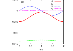
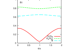
Fig. 3: $\theta$ dependence of (a) the order parameters and (b) the effective quark mass $\Pi_{f}$ at $T=163$ MeV and $\mu=0$ in the EPNJL model. In panel (b), $\Pi_{f}$ is normalized by the value at $T=\mu=\theta=0$ and the normalized $\Pi_{f}$ is compared with the Polyakov loop $\Phi$. See the legend for the definition of lines.

Figure 4 shows $T$ dependence of the order parameters at $\theta=\pi$ and $\mu=0$. Comparing this figure with Fig. 1, one can also see $\theta$ dependence of the order parameters. In the PNJL model of panel (a), $|\eta_{l}|$ and $|\eta_{s}|$ are finite below the critical temperature $T_{P}=194$ MeV and vanish above $T_{P}$. Thus the $P$ symmetry is broken at smaller $T$, but restored at higher $T$. In the two-flavor PNJL model, this $P$ restoration is second order Sakai et al (2011). This is the case also for the present 2+1 flavor PNJL model. The second order $P$ restoration induces cusps in $|\sigma_{l}|$ and $|\sigma_{s}|$ when $T=T_{P}$, although the cusp is weak in $|\sigma_{s}|$. This propagation of the cusp can be understood by the extended discontinuity theorem of Ref. Kasihwa et al (2009). In the EPNJL model of panel (b), the $P$ restoration occurs at $T_{P}=158$ MeV as the first-order transition. The same property is seen in the two-flavor EPNJL model Sakai et al (2011). The first-order $P$ restoration generates gaps in $|\sigma_{l}|$ and $|\sigma_{s}|$ when $T=T_{P}$, although the gap is tiny in $|\sigma_{s}|$. This propagation of the gap can be understood by the discontinuity theorem by Barducci, Casalbuoni, Pettini and Gatto Barducci et al. (1993). Thus the Dashen phenomena are seen only at lower $T$, and the order of the $P$ violation at the critical temperature $T_{P}$ depends on the effective model taken.

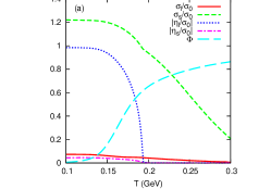
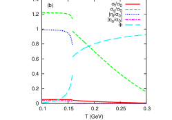
Fig. 4: $T$ dependence of the order parameters at $\theta=\pi$ and $\mu=0$ in (a) the PNJL model and (b) the EPNJL model. See the legend for the definition of lines.

Theoretical prediction on the critical temperature of the chiral transition at $\theta=0$ and $\mu=0$ and the P restoration at $\theta=\pi$ and $\mu=0$ is tabulated in Table 3. At $\theta=0$, the chiral transition is crossover in all of the NJL, PNJL, and EPNJL models At $\theta=\pi$, the order of the P restoration is first order in the EPNJL model, but it is second order in the PNJL and NJL models.

Model	$\theta=0$	$\theta=\pi$
NJL	$177$ (crossover)	$170$ (2nd order)
PNJL	$200$ (crossover)	$194$ (2nd order)
EPNJL	$162$ (crossover)	$158$ (1st order)

Table 3: Theoretical prediction on the critical temperature of the chiral transition at $\theta=0$ and $\mu=0$ and the P restoration at $\theta=\pi$ and $\mu=0$. The values are shown in units of MeV.

III.2 Thermodynamics at $\mu>0$

In this subsection, we consider the case of $\mu>0$ where $C$ symmetry is not exact. In general, the relation $\Phi=\Phi^{*}$ is not satisfied for finite $\mu$, although $\Phi$ and $\Phi^{*}$ are real Sasaki et al. (2010). This situation makes numerical calculations quite time-consuming. However, the deviation $\Phi-\Phi^{*}$ is known to be very small Sasaki et al. (2010). For this reason, the assumption $\Phi=\Phi^{*}$ has been used in many calculations. Therefore we use the assumption also in this paper.

Figure 5 represents $T$ dependence of the order parameters at $\theta=\pi$ and $\mu=300$ MeV in the PNJL and EPNJL models. The $P$ restoration takes place at high $T$, since $\eta_{l}$ and $\eta_{s}$ are zero there. The critical temperature of the $P$ restoration is $T_{P}=110$ MeV for the PNJL model and $T_{P}=99$ MeV for the EPNJL model. For $\mu=300$ MeV, the order of the $P$ restoration at $T=T_{P}$ is first order in both the PNJL and EPNJL models. Thus the quark-number chemical potential $\mu$ lowers $T_{P}$ and makes the $P$ restoration sharper.

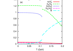
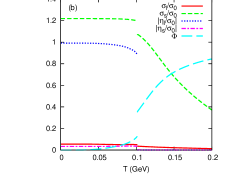
Fig. 5: $T$ dependence of the order parameters at $\theta=\pi$ and $\mu=300$ MeV in (a) the PNJL model and (b) the EPNJL model. See the legend for the definition of lines.

Figure 6 shows the phase diagram of the chiral transition in the $\mu$-$\theta$-$T$ space. The diagram is mirror symmetric with respect to the $\mu$-$T$ plane at $\theta=0$, so the diagram is plotted only at $\theta\geq 0$. Panels (a) and (b) correspond to results of the PNJL and EPNJL models, respectively. In the $\mu$-$T$ plane at $0\leq\theta<\pi$, the solid line stands for the first-order chiral transition, while the dashed line represents the chiral crossover. The meeting point between the solid and dashed lines is a critical endpoint (CEP) of second order. Point C is a CEP in the $\mu$-$T$ plane at $\theta=0$ Asakawa and Yazaki (1989); Barducci et al. (2006). For both the PNJL and EPNJL models, the location of CEP in the $\mu$-$T$ plane moves to higher $T$ and lower $\mu$ as $\theta$ increases from 0 to $\pi$.

In the $\mu$-$T$ plane at $\theta=\pi$, $P$ symmetry is exact and hence we can consider the spontaneous breaking of $P$ symmetry in addition to the chiral transition. For the PNJL model of panel (a), both the first-order chiral transition and the first-order $P$ restoration take place simultaneously, and the second-order $P$ restoration and the chiral crossover coincide with each other. The first-order and the second-order $P$ transition line are depicted by the solid and dashed lines, respectively. The meeting point A is a tricritical point (TCP) of the $P$-restoration transition. For the EPNJL model of panel (b), the chiral and the $P$ restoration transition are always first order and hence there is no TCP.

In the PNJL model of panel (a), the dotted line from point C to point A is a trajectory of CEP as $\theta$ increases from 0 to $\pi$. Thus the second-order chiral transition line ends up with point A. This means that the CEP (point C) at $\theta=0$ is a remnant of the TCP (point A) of $P$ restoration at $\theta=\pi$. In the EPNJL model of panel (b), no TCP and then no CEP appears in the $\mu$-$T$ plane at $\theta=\pi$. The second-order chiral-transition line (dashed line) starting from point C never reaches the $\mu$-$T$ plane at $\theta=\pi$.

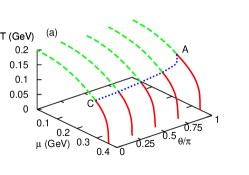
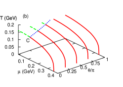
Fig. 6: Phase diagram of the chiral transition in the $\mu$-$\theta$-$T$ space. Panel (a) shows a result of the PNJL model and panel (b) corresponds to a result of the EPNJL model.

Figure 7 snows the projection of the second-order chiral-transition line in the $\mu$-$\theta$-$T$ space on the $\mu$-$\theta$ plane. The solid (dashed) line stands for the projected line in the EPNJL (PNJL) model. The first-order transition region exists on the right-hand side of the line, while the left-hand side corresponds to the chiral crossover region. The first-order transition region is much wider in the EPNJL model than in the PNJL model. In the EPNJL model, eventually, the chiral transition becomes first order even at $\mu=0$ when $\theta$ is large.

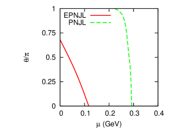
Fig. 7: The projection of the second-order chiral-transition line in the $\mu$-$\theta$-$T$ space on the $\mu$-$\theta$ plane. See the legend for the definition of line.

III.3 The sign problem on LQCD with finite $\theta$

In the PNJL Lagrangian (16) after the transformation (2), $\theta$ dependence appears only at the light quark mass terms, $m_{l}\cos(\theta/2)$ and $m_{l}\sin(\theta/2)$. These terms are much smaller than $\Lambda_{QCD}$ as a typical scale of QCD. This means that the condensates, $\sigma_{l}^{\prime}$, $\sigma_{s}^{\prime}$, $\eta_{l}^{\prime}$ and $\eta_{s}^{\prime}$, have weak $\theta$ dependence. This statement is supported by the results of the PNJL calculations shown in Fig. 8.

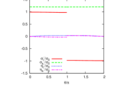
Fig. 8: $\theta$ dependence of the order parameters, $\sigma_{l}^{\prime}$, $\sigma_{s}^{\prime}$, $\eta_{l}^{\prime}$ and $\eta_{s}^{\prime}$, at $T=\mu=0$ calculated with the EPNJL model. See the legend for the definition of lines.

The sign problem is induced by the $\theta$ odd $m_{l}\sin(\theta/2)$ term. The $\theta$-odd ($P$-odd) condensates, $\eta_{l}^{\prime}$ and $\eta_{s}^{\prime}$, are generated by the $\theta$-odd mass term. One can see in Fig. 8 that the $\theta$-odd condensates are much smaller than the $\theta$-even condensates, $\sigma_{l}^{\prime}$ and $\sigma_{s}^{\prime}$. This fact indicates that effects of the $\theta$-odd mass term are negligible. Actually, if the term is neglected, the $\theta$-even condensates change only within the thickness of line, while the $\theta$-odd condensates vanish. The neglect of the $\theta$-odd mass is thus a good approximation.

The validity of the approximation can be shown more explicitly in the following way. The $\theta$-odd ($P$-odd) condensates, $\eta_{l}^{\prime}$ and $\eta_{s}^{\prime}$, are zero at $\theta=0$, since the $\theta$-odd mass vanishes there. The weak $\theta$ dependence of $\eta_{l}^{\prime}$ and $\eta_{s}^{\prime}$ guarantees that $\eta_{l}^{\prime}$ and $\eta_{s}^{\prime}$ are small for any $\theta$. Setting $\eta_{l}^{\prime}=\eta_{s}^{\prime}=0$ in $M^{\prime}_{l}$ and $N_{l}^{\prime}$ leads to

$$M_{l}^{\prime} = \cos{\left(\tfrac{\theta}{2}\right)}m_{l}-4G_{\rm S}\sigma^{\prime}_{l}+2G_{\rm D}\sigma^{\prime}_{s}\sigma^{\prime}_{l},$$ (28)

$$N_{l}^{\prime} = \sin{\left(\tfrac{\theta}{2}\right)}m_{l},$$ (29)

where $M_{l}^{\prime}\approx\Lambda_{\rm QCD}$ and $N_{l}^{\prime}\approx m_{l}$. Since the thermodynamic potential is a function of $M_{l}^{\prime 2}+N_{l}^{\prime 2}$, the term $N_{l}^{\prime 2}$ is negligible compared with $M_{l}^{\prime 2}$.

In LQCD, the vacuum expectation value of operator ${\cal O}$ is obtained by

$$\langle{\cal O}\rangle = \int\mathcal{D}A{\cal O}\left({\rm det}{\cal M}_{l}(\theta)\right)^{2}{\rm det}{\cal M}_{s}e^{-S_{g}}$$ (30)

$$= \int\mathcal{D}A{\cal O}^{\prime}\left({\rm det}{\cal M}_{l}^{\prime}(\theta)\right)^{2}{\rm det}{\cal M}_{s}e^{-S_{g}}$$ (31)

with the gluon part $S_{g}$ of the QCD action and

$${\cal O}^{\prime}\equiv{\cal O}\frac{\left({\rm det}{\cal M}_{l}(\theta)\right)^{2}}{\left({\rm det}{\cal M}_{l}^{\prime}(\theta)\right)^{2}},$$ (32)

where ${\rm det}{\cal M}^{\prime}_{l}(\theta)$  is the Fermion determinant in which the $\theta$-odd mass is neglected and hence has no sign problem. As mentioned above, one can assume that

$$\frac{{\rm det}{\cal M}_{l}(\theta)}{{\rm det}{\cal M}^{\prime}_{l}(\theta)}\approx 1.$$ (33)

Thus the reweighting method defined by (31) may work well. In the $\theta$-even mass, $m_{l}\cos(\theta/2)$, the limit of $\theta=\pi$ corresponds to the limit of $m_{l}=0$ with $m_{s}$ fixed. Although the limit is hard to reach, one can analyze the dynamics at least at small and intermediate $\theta$.

IV Summary

We have investigated effects of the theta vacuum on the QCD phase diagram for the realistic 2+1 flavor system, using the three-flavor PNJL and EPNJL models. The effects can be easily understood by the $SU_{\rm A}(3)\otimes U_{\rm A}(1)$ transformation (2). After the transformation, the $\theta$-odd mass, $m_{l}\sin(\theta/2)$, little affects the dynamics, so that the dynamics is mainly governed by the $\theta$-even mass, $m_{l}\cos(\theta/2)$. In the $\theta$-even mass, the increase of $\theta$ corresponds to the decrease of $m_{l}$ with $m_{s}$ fixed. This means that the chiral transition becomes strong as $\theta$ increases. This is true in the results of both PNJL and EPNJL calculations. Particularly in the EPNJL model that is more reliable than the PNJL model, the transition becomes first-order even at $\mu=0$ when $\theta$ is large. This result is important. If the chiral transition becomes first order at $\mu=0$, it will change the scenario of cosmological evolution. For example, the first-order transition allows us to think the inhomogeneous Big-Bang nucleosynthesis model or a new scenario of baryogenesis.

Using the fact that the $\theta$-odd mass is negligible, we have proposed a way of circumventing the sign problem on LQCD with finite $\theta$. The reweighting method by defined (31) may allow us to do LQCD calculations and get definite results on the dynamics of the $\theta$ vacuum.

- (1) C. G. Callan, R. F. Dashen, and D. J. Gross, Phys. Lett. B63, 334 (1976); J. Jackiw, and C. Rabbi, Phys. Rev. Lett. 37, 172 (1976).
- (2) C. A. Baker, et al., Phys. Rev. Lett. 97, 131801 (2006).
- (3) K. Kawarabayashi and N. Ohta, Nucl. Phys. B175, 477 (1980); Prog. Theor. Phys. 66, 1789 (1981); N. Ohta, Prog. Theor. Phys. 66, 1408 (1981); [Erratum-ibid. 67 (1982) 993].
- (4) E. Vicari and H. Panagopoulos, Phys. Rept. 470, 93 (2009).
- (5) L. McLerran, E. Mottola and M. E. Shaposhnikov, Phys. Rev. D 43, 2027 (1991).
- Kharzeev and Zhitnitsky (2007) D. Kharzeev, and A. Zhitnitsky, Nucl. Phys. A 797, 67 (2007).
- Metlitski and Zhitnitsky (2005) M. A. Metlitski, and A. R. Zhitnitsky, Nucl. Phys. B731, 309 (2005); Phys. Lett. B 633, 721 (2006).
- (8) R. D. Peccei and H. R. Quinn, Phys. Rev. D 16, 1791 (1977).
- (9) J. W. Kim, Phys. Rev. Lett. 43, 103 (1979).
- (10) M. A. Shifman A. I. Vainstein and V. I. Zakharov, Nucl. Phys. B 166, 493 (1980).
- (11) A. R. Zhitnitsky, Sov. J. Nucl. Phys. 31, 260 (1980).
- (12) M. Dine W. Fischler and M. Srednicki, Phys. Lett. B 104, 199 (1981).
- (13) D. Kharzeev, Phys. Lett. B 633, 260 (2006); D. Kharzeev, L. D. McLerran, and H. J. Warringa, Nucl. Phys. A 803, 227 (2008).
- (14) K. Fukushima, D. E. Kharzeev, and H. J. Warringa, Phys. Rev. D 78, 074033 (2008).
- Fukushima et al. (2010) K. Fukushima, M. Ruggieri, and R. Gatto, Phys. Rev. D 81, 114031 (2010).
- (16) B. I. Abelev et al. [STAR Collaboration], Phys. Rev. Lett. 103, 251601 (2009); Phys. Rev. C 81, 054908 (2010).
- (17) C. Vafa and E. Witten, Phys. Rev. Lett. 53, 535 (1984).
- (18) R. Dashen, Phys. Rev. D 3, 1879 (1971).
- Witten (1980) E. Witten, Ann. Phys. 128, 363 (1980).
- Vecchia and Veneziano (1980) P. di Vecchia, and G. Veneziano, Nucl. Phys. B171, 253 (1980).
- (21) A. V. Smilga, Phys. Rev. D 59, 114021 (1999).
- (22) M. H. G. Tytgat, Phys. Rev. D 61, 114009 (2000).
- (23) G. Akemann, J. T. Lenaghan, and, K. Splittorff, Phys. Rev. D 65, 085015 (2002).
- (24) M. Creutz, Phys. Rev. Lett. 92, 201601 (2004).
- Fujihara et al. (2010) T. Fujihara, T. Inagaki, and D. Kimura, Prog. Theor. Phys. 117, 139 (2007).
- Boer and Boomsma (2008a) D. Boer and J. K. Boomsma, Phys. Rev. D 78, 054027 (2008).
- Boomsma and Boer (2008a) J. K. Boomsma and D. Boer, Phys. Rev. D 80, 034019 (2009).
- Chatteriee et al (2011) B. Chatteriee, H. Mishra and A. Mishra, arXiv:1111.4061 [hep-ph](2011).
- Kouno et al (2011) H. Kouno, Y. Sakai, T. Sasaki, K. Kashiwa, and M. Yahiro, Phys. Rev. D 83, 076009 (2011).
- Sakai et al (2011) Y. Sakai, H. Kouno, T. Sasaki, and M. Yahiro, Phys. Lett. B 705, 349 (2011).
- Nambu and Jona-Lasinio (1961a) Y. Nambu and G. Jona-Lasinio, Phys. Rev. 122, 345 (1961); Phys. Rev. 124, 246 (1961).
- Asakawa and Yazaki (1989) M. Asakawa and K. Yazaki, Nucl. Phys. A504, 668 (1989).
- Kashiwa et al (2006) K. Kashiwa, H. Kouno, T. Sakaguchi, M. Matsuzaki, and M. Yahiro, Phys. Lett. B 647, 446 (2007); K. Kashiwa, M. Matsuzaki, H. Kouno, and M. Yahiro, Phys. Lett. B 657, 143 (2007).
- Matsumoto (2010) T. Matsumoto, K. Kashiwa, H. Kouno, K. Oda, and M. Yahiro, Phys. Lett. B 694, 367 (2011).
- Sasaki et al. (2011) T. Sasaki, Y. Sakai, H. Kouno, and M. Yahiro, Phys. Rev. D 84, 091901 (2011);
- ’t Hooft (1976) G. ’t Hooft, Phys. Rev. Lett. 37, 8 (1976); Phys. Rev. D 14, 3432 (1976); 18, 2199(E) (1978).
- Kobayashi and Maskawa (1970) M. Kobayashi, and T. Maskawa, Prog. Theor. Phys. 44, 1422 (1970); M. Kobayashi, H. Kondo, and T. Maskawa, Prog. Theor. Phys. 45, 1955 (1971).
- Meisinger et al. (1996) P. N. Meisinger, and M. C. Ogilvie, Phys. Lett. B 379, 163 (1996).
- Fukushima (2004) K. Fukushima, Phys. Lett. B 591, 277 (2004); Phys. Rev. D 77, 114028 (2008).
- Ratti et al. (2006) C. Ratti, M. A. Thaler, and W. Weise, Phys. Rev. D 73, 014019 (2006).
- Rossner et al. (2007) S. Rößner, C. Ratti, and W. Weise, Phys. Rev. D 75, 034007 (2007).
- Schaefer (2007) B. -J. Schaefer, J. M. Pawlowski, and J. Wambach, Phys. Rev. D 76, 074023 (2007).
- Kashiwa et al (2008) K. Kashiwa, H. Kouno, M. Matsuzaki, and M. Yahiro, Phys. Lett. B 662, 26 (2008).
- Sakai et al (2008) Y. Sakai, K. Kashiwa, H. Kouno, and M. Yahiro, Phys. Rev. D 77, 051901(R) (2008); Phys. Rev. D 78, 036001 (2008); Y. Sakai, K. Kashiwa, H. Kouno, M. Matsuzaki, and M. Yahiro, Phys. Rev. D 78, 076007 (2008); K. Kashiwa, M. Matsuzaki, H. Kouno, Y. Sakai, and M. Yahiro, Phys. Rev. D 79, 076008 (2009); K. Kashiwa, H. Kouno, and M. Yahiro, Phys. Rev. D 80, 117901 (2009).
- Sakai et al (2008) Y. Sakai, K. Kashiwa, H. Kouno, M. Matsuzaki, and M. Yahiro, Phys. Rev. D 79, 096001 (2009);
- Kahara (2009) T. Kähärä, and K. Tuominen, Phys. Rev. D 80, 114022 (2009).
- Kasihwa et al (2009) K. Kashiwa, M. Yahiro, H. Kouno, M. Matsuzaki, and Y. Sakai, J. Phys. G: Nucl. Part. Phys. 36, 105001 (2009).
- Kouno et al (2009) H. Kouno, Y. Sakai, K. Kashiwa, and M. Yahiro, J. Phys. G: Nucl. Part. Phys. 36, 115010 (2009).
- Sasaki et al. (2009) T. Sasaki, Y. Sakai, H. Kouno, and M. Yahiro, Phys. Rev. D 82, 116004 (2010); Y. Sakai, H. Kouno, and M. Yahiro, J. Phys. G: Nucl. Part. Phys. 37, 105007 (2010).
- Sasaki et al. (2010) Y. Sakai, T. Sasaki, H. Kouno, and M. Yahiro, Phys. Rev. D 82, 096007 (2010).
- Sakai (2010) Y. Sakai, T. Sasaki, H. Kouno, and M. Yahiro, Phys. Rev. D 82, 076003 (2010); arXiv:1104.2394 [hep-ph] (2011).
- Gatto (2011) R. Gatto, and M. Ruggieri, Phys. Rev. D 83, 034016 (2011).
- Soeldner (2010) W. Söldner, arXiv:1012.4484 [hep-lat] (2010).
- Kanaya (2010) K. Kanaya, arXiv:hep-ph/1012.4235 [hep-ph] (2010); arXiv:hep-ph/1012.4247 [hep-lat] (2010).
- Borsanyi etal (2010) S. Borsányi, Z. Fodor, C. Hoelbling, S. D. Katz, S. Krieg, C. Ratti, and K. K. Szabo, arXiv:1005.3508 [hep-lat] (2010).
- (56) P. Rehberg, S.P. Klevansky and J. Hüfner, Phys. Rev. C 53, 410 (1996); S.P. Klevansky, Rev. Mod. Phys. 64, 649 (1992).
- Roberge and Weiss (1986) A. Roberge and N. Weiss, Nucl. Phys. B275, 734 (1986).
- Kondo (2010) K.-I. Kondo, Phys. Rev. D 82, 065024 (2010).
- Braun (2010) J. Braun, L. M. Haas, F. Marhauser, and J. M. Pawlowski, Phys. Rev. Lett. 106, 022002 (2011); J. Braun, and A. Janot, arXiv:1102.4841 [hep-ph] (2011).
- Wetterich (1993) C. Wetterich, Phys. Lett. B 301, 90 (1993).
- (61) Y. Aoki, G. Endrödi, Z. Fodor, S. D. Katz and K. K. Szabó, Nature 443, 675 (2006).
- FP2010 (2009) P. de Forcrand and O. Philipsen, arXiv:1004.3144 [hep-lat](2010).
- Barducci et al. (1993) A. Barducci, R. Casalbuoni, G. Pettini, and R. Gatto, Phys. Lett. B 301, 95 (1993).
- Barducci et al. (2006) A. Barducci, R. Casalbuoni, S. De Curtis, R. Gatto, and G. Pettini, Phys. Lett. B 231, 463 (1989); A. Barducci, R. Casalbuoni, G. Pettini, and R. Gatto, Phys. Rev. D 49, 426 (1994);