Effects of Primordial Magnetic Field with Log-normal Distribution on Cosmic Microwave Background

Abstract

We study the effect of primordial magnetic fields (PMFs) on the anisotropies of the cosmic microwave background (CMB). We assume the spectrum of PMFs is described by log-normal distribution which has a characteristic scale, rather than power-law spectrum. This scale is expected to reflect the generation mechanisms and our analysis is complementary to previous studies with power-law spectrum. We calculate power spectra of energy density and Lorentz force of the log-normal PMFs, and then calculate CMB temperature and polarization angular power spectra from scalar, vector, and tensor modes of perturbations generated from such PMFs. By comparing these spectra with WMAP7, QUaD, CBI, Boomerang, and ACBAR data sets, we find that the current CMB data set places the strongest constraint at $k\simeq 10^{-2.5}$ Mpc^-1 with the upper limit $B\lesssim 3$ nG.

I Introduction

Many researchers have studied magnetic fields for wider ranges in the early Universe. Recently, magnetic fields with strength $\sim 1\mu$ G have been observed in clusters of galaxies, and primordial magnetic fields (PMFs) have been studied by many authors to explain their origins. The strength of PMFs is constrained as $B\lesssim 1$ nG from cosmological observations, such as temperature and polarization anisotropies of cosmic microwave background (CMB) and matter power spectra Subramanian and Barrow (1998); Mack et al. (2002); Subramanian and Barrow (2002); Lewis (2004); Yamazaki et al. (2005a); Kahniashvili and Ratra (2005); Challinor (2004); Dolgov (2005); Gopal and Sethi (2005); Yamazaki et al. (2005b); Kahniashvili and Ratra (2007); Yamazaki et al. (2006a, b, c); Giovannini (2006a); Yamazaki et al. (2008); Paoletti et al. (2009); Finelli et al. (2008); Yamazaki et al. (2008, 2008); Sethi et al. (2008); Kojima et al. (2008); Kahniashvili et al. (2008); Giovannini and Kunze (2008); Yamazaki et al. (2009); Shaw and Lewis (2010); Yamazaki et al. (2010a, b, c).

Many theoretical models have been proposed for generating PMFs of cosmological scales. Generation models of PMFs from inflation can create strong fields, whose amplitude is of the order of $1$ nG at redshift $z\sim 0$, depending on assumed hypothetical fields and couplings Turner and Widrow (1988); Ratra (1992); Bamba and Yokoyama (2004, 2004); Bamba and Sasaki (2007). Furthermore, PMFs can be generated by primordial perturbations of density fields Takahashi et al. (2005); Ichiki et al. (2006), the Beiermann battery mechanism in primordial supernovae remnants Hanayama et al. (2005) or the Weibel instabilities Fujita and Kato (2005). These PMFs can evolve into the magnetic fields observed in galaxies and/or galaxy clusters directly or through the dynamo process.

While magnetogenesis during inflation can produce PMFs beyond the horizon scale, PMFs generated by the other mechanism are expected to have the characteristic scale because they are based on causal processes. Here it should be noted that the coherence length of PMFs can grow after generation due to inverse cascade Christensson et al. (2001); Banerjee and Jedamzik (2004), although the efficiency is still under study.

In the previous studies to put constraints on PMFs from CMB anisotropies, the spectrum of PMFs was assumed to be power-law shape. Although power-law spectrum is natural for magnetogenesis during inflation, this is not the case for the other mechanisms based on causal processes. Furthermore, in previous studies with power-law PMFs, it was not so clear which scale of PMFs mainly contributes to the constraints. Since inflationary mechanisms tend to generate power-law magnetic fields, the magnetic fields which have a characteristic scale at cosmological scales are difficult to be produced and seem somewhat artificial. However, it is still possible that such fields can be constrained by observation, and if observed it would give us useful information about generation mechanism of cosmological magnetic fields. Hence, in this article, as a toy example we use a log-normal distribution (LND) for the PMF spectrum $f_{\mathrm{LND}}(k;k_{\mathrm{M}},\sigma_{\mathrm{M}})$ which has a characteristic scale expressed by $k_{\mathrm{M}}$, and aim to constrain PMFs scale by scale instead of the power-law PMF spectrum. These quantities reflect the generation mechanism but here we regard them just as parameters. We study features of angular power spectra of the CMB from the PMFs with log-normal distribution. Finally we constrain the strength of the PMFs for fixed sets of the parameters.

II Power Spectrum of PMF

The electromagnetic tensor has the usual form

$${F^{\alpha}}_{\beta}=\left(\begin{array}[]{cccc}0&E_{1}&E_{2}&E_{3}\\ E_{1}&0&-B_{3}&B_{2}\\ E_{2}&B_{3}&0&-B_{1}\\ E_{3}&-B_{2}&B_{1}&0\\ \end{array}\right)~{}~{},$$ (5)

where $E_{i}$ and $B_{i}$ are the electric and magnetic fields. Here we use natural units $c=\hbar=1$. The energy-momentum tensor for electromagnetism is

$${T^{\alpha\beta}}_{[\mathrm{EM}]}=\frac{1}{4\pi}\left(F^{\alpha\gamma}F^{\beta}_{\gamma}-\frac{1}{4}g^{\alpha\beta}F_{\gamma\delta}F^{\gamma\delta}\right).$$ (6)

The Maxwell stress tensor, $\sigma^{ik}$ is derived from the space-space components of the electromagnetic energy-momentum tensor,

$$-{T^{ik}}_{[\mathrm{EM}]}=\sigma^{ik}=\frac{1}{4\pi a^{2}}\left\{E^{i}E^{k}+B^{i}B^{k}-\frac{1}{2}\delta^{ik}(E^{2}+B^{2})\right\}.$$ (7)

where $a$ is the cosmic scale factor.

We consider the case that the spectrum of the PMFs at large scales had been well established before the CMB epoch, after their generation and followed by perhaps a complicated time evolution. In this case we do not need to consider the time evolution of magnetic fields in our CMB analysis, e.g. nonliner effects Banerjee and Jedamzik (2004), of the PMF and we consider only the dilution due to the expansion of the Universe. Within the linear approximation Durrer et al. (2000) we can discard the MHD backreaction onto the field itself. The conductivity of the primordial plasma is very large, and magnetic fields are frozen in the plasma Mack et al. (2002). This is a very good approximation during the epochs of interest here. Furthermore, we can neglect the electric field, i.e. $E\sim 0$, and can decouple the time evolution of the magnetic field from its spatial dependence, i.e. $\mathbf{B}(\tau,\mathbf{x})=\mathbf{B}(\mathbf{x})/a^{2}$ for very large scales. In this way we obtain the following equations,

$${T^{00}}_{[\mathrm{EM}]}=\frac{B^{2}}{8\pi a^{6}}~{}~{},$$ (8)

$${T^{i0}}_{[\mathrm{EM}]}={T^{0k}}_{[\mathrm{EM}]}=0~{}~{},$$ (9)

$$-{T^{ik}}_{[\mathrm{EM}]}=\sigma^{ik}=\frac{1}{8\pi a^{6}}(2B^{i}B^{k}-\delta^{ik}B^{2})~{}~{}.$$ (10)

II.1 power spectra of PMFs from the log-normal distribution

We defined a two point correlation function of the PMFs as follows,

$$\left\langle B^{i}(\mbox{k}){B^{j}}^{*}(\mbox{k}^{\prime})\right\rangle = (2\pi)^{3}P_{\mathrm{[PMF]}}(k)P^{ij}(k)\delta(\mbox{k}-\mbox{k}^{\prime})~{},$$ (11)

where

$$P^{ij}(k) = \delta^{ij}-\frac{k{}^{i}k{}^{j}}{k{}^{2}}.$$ (12)

We follow the convention for the Fourier transform as

$$f(\mbox{k})=\int d^{3}x\exp(i\mbox{k}\cdot\mbox{x})F(\mbox{x}).$$ (13)

If PMFs have been generated from inflation the power-law model would be a good representation of the magnetic field power spectrum. On the other hand, if the PMFs were created through mechanisms other than inflation, the spectrum would have a characteristic scale and may not be described as a simple power-law.

Furthermore, we need to understand how such PMFs cascade from smaller to larger scales to study effects of the PMFs created in the early Universe on the large-scale structures. Actually, we can learn behaviors of PMF cascading or inverse cascading by simulationsKahniashvili et al. (2010), whose results, however, generally depend on cosmological parameters and models. Since such simulations generally take too much time and have a limited dynamical range, it is not efficient to estimate distributions of the PMF by some simulations when we study cosmology and astrophysics with the PMF quantitatively.

To avoid these problems, we use in place of the power law a LND defined as,

$$f_{\mathrm{LND}}(k;k_{\mathrm{M}},\sigma_{\mathrm{M}})=\frac{1}{k\sigma_{\mathrm{M}}\sqrt{2\pi}}\exp\left\{-\frac{\left[\ln{(k)}-\ln{(k_{\mathrm{M}})}\right]^{2}}{2\sigma_{\mathrm{M}}^{2}}\right\},$$ (14)

where $k_{\mathrm{M}}$ is the characteristic scale depending on the PMF generation model, and $\sigma_{\mathrm{M}}$ is the variance. The variance $\sigma_{\mathrm{M}}$ in Eq.(14) expresses how this distribution is expanded (or concentrated) around the characteristic scale $k_{\mathrm{M}}$. Therefore, the variance $\sigma_{\mathrm{M}}$ may be related to the cascading of the PMFs. Using Eq.(14), the power spectrum of the PMF is given by

$$P_{\mathrm{[PMF]}}(k)=Af_{\mathrm{[LND]}}(k;k_{\mathrm{M}},\sigma_{\mathrm{M}}).$$ (15)

We shall determine the coefficient from the variance of magnetic fields in real space,

$$\left.\left\langle B^{i}(\mbox{x}){B^{i}}(\mbox{x})\right\rangle\right|_{d}=B_{d}^{2}$$ (16)

where $d=2\pi/k_{\mathrm{M}}$ and

$$\left\langle B^{i}(\mbox{x}){B^{j\ast}}(\mbox{x}^{\prime})\right\rangle=\frac{1}{(2\pi)^{6}}\int d^{3}k\int d^{3}k^{\prime}\exp(-i\mbox{x}\cdot\mbox{k}+i\mbox{x}^{\prime}\cdot\mbox{k}^{\prime})\left\langle B^{i}(\mbox{k}){B^{j\ast}}(\mbox{k}^{\prime})\times w(k)\right\rangle.$$ (17)

The window function $w(k)$ is given by the rectangular function as $w(k)=1$ for $k_{-}<k<k_{+}$ and $w(k)=0$ for otherwise. Here,

$$\left\{\begin{array}[]{l}k_{+}=\exp{(\ln{k_{\mathrm{M}}}+n\sigma_{\mathrm{M}})}={10^{\frac{\ln{k_{\mathrm{M}}}+n\sigma_{\mathrm{M}}}{\ln{(10)}}}},\\ k_{-}=\exp{(\ln{k_{\mathrm{M}}}-n\sigma_{\mathrm{M}})}={10^{\frac{\ln{k_{\mathrm{M}}}-n\sigma_{\mathrm{M}}}{\ln{(10)}}}},\end{array}\right.$$ (20)

where $n$ gives the range of integration. From Eq.(17), we obtain the amplitude of the log-normal distribution as

$$A=B^{2}_{\mathrm{d}}\frac{(2\pi)^{2}}{4}\left\{\int^{k_{+}}_{k_{-}}dkk\frac{1}{\sigma_{\mathrm{M}}\sqrt{2\pi}}\exp{\left[-\frac{(\ln|k|-\ln|k_{\mathrm{M}}|)^{2}}{2\sigma_{\mathrm{M}}^{2}}\right]}\right\}^{-1}.$$ (21)

As mentioned above, we can neglect the diffusion of the magnetic field at cosmological scales for the age of the Universe. Therefore we can assume that the energy of the LND-PMF is not dissipated; in other words, the integral of Eq.(11) over $k$ from $k_{-}$ to $k_{+}$ is time-independent. In this case, $k_{-}$ and $k_{+}$ should be taken to be $\pm$ infinites. In practice, we take $k_{-}$ and $k_{+}$ far enough from the peak of the distribution .

Using Eq.(14) and the method presented by Ref.Yamazaki et al. (2006a); Yamazaki et al. (2008), we obtain power spectra from the LND function for each perturbation mode as follows. For the scalar mode, the power spectrum of the energy (pressure) of the PMFs is

$$P_{\mathrm{[EM:SE]}}(k;k_{\mathrm{M}},\sigma_{\mathrm{M}})= \frac{A^{2}}{8(2\pi)^{4}a^{8}}\int dk^{\prime}{k^{\prime}}^{2}\int^{1}_{-1}d\mathcal{C}f_{\mathrm{LND}}(|k^{\prime}|;k_{\mathrm{M}},\sigma_{\mathrm{M}})f_{\mathrm{M}}(|k-k^{\prime}|;k_{\mathrm{M}},\sigma_{\mathrm{M}})$$

$$\times\frac{\left\{(1+\mathcal{C}^{2})k^{2}-4kk^{\prime}\mathcal{C}+2{k^{\prime}}^{2}\right\}}{|\mbox{k}-\mbox{k}^{\prime}|^{2}}~{},$$

the power spectrum of the magnetic tension is

$$P_{\mathrm{[EM:ST]}}(k;k_{\mathrm{M}},\sigma_{\mathrm{M}})= \frac{A^{2}}{2(2\pi)^{4}a^{8}}\int dk^{\prime}k^{\prime}{}^{2}\int^{1}_{-1}d\mathcal{C}f_{\mathrm{M}}(|k^{\prime}|;k_{\mathrm{M}},\sigma_{\mathrm{M}})f_{\mathrm{M}}(|k-k^{\prime}|;k_{\mathrm{M}},\sigma_{\mathrm{M}})$$

$$\times\frac{k^{\prime}{}^{2}}{|\mbox{k}-\mbox{k}^{\prime}|^{2}}\left(1-\mathcal{C}^{2}\right)^{2}~{},$$

and the correlation term between the energy and tension is

$$P_{\mathrm{[EM:SET]}}(k;k_{\mathrm{M}},\sigma_{\mathrm{M}})= \frac{A^{2}}{4(2\pi)^{4}a^{8}}\int dk^{\prime}{k^{\prime}}^{2}\int^{1}_{-1}d\mathcal{C}f_{\mathrm{LND}}(|k^{\prime}|;k_{\mathrm{M}},\sigma_{\mathrm{M}})f_{\mathrm{LND}}(|k-k^{\prime}|;k_{\mathrm{M}},\sigma_{\mathrm{M}})$$

$$\times\frac{k^{\prime}(1-\mathcal{C}^{2})}{|\mbox{k}-\mbox{k}^{\prime}|^{2}}(k^{\prime}-k\mathcal{C})~{}.$$

For the vector mode, the power spectrum of the PMFs is;

$$P_{\mathrm{[EM:V]}}(k;k_{\mathrm{M}},\sigma_{\mathrm{M}})= \frac{A^{2}}{8(2\pi)^{4}a^{8}}\int dk^{\prime}k^{\prime}{}^{2}\int^{1}_{-1}d\mathcal{C}f_{\mathrm{LND}}(|k^{\prime}|;k_{\mathrm{M}},\sigma_{\mathrm{M}})f_{\mathrm{LND}}(|k-k^{\prime}|;k_{\mathrm{M}},\sigma_{\mathrm{M}})$$

$$\times\frac{(1-C^{2})}{|\mbox{k}-\mbox{k}^{\prime}|^{2}}\left\{2k^{2}-5Ckk^{\prime}+(2C^{2}+1)k^{\prime}{}^{2}\right\}~{}.$$

Finally, for the tensor mode the power spectrum of anisotropic stress of the PMFs is found to be

$$P_{\mathrm{[EM:T]}}(k;k_{\mathrm{M}},\sigma_{\mathrm{M}})= \frac{A^{2}}{16(2\pi)^{4}a^{8}}\int dk^{\prime}k^{\prime}{}^{2}\int^{1}_{-1}d\mathcal{C}f_{\mathrm{LND}}(|k^{\prime}|;k_{\mathrm{M}},\sigma_{\mathrm{M}})f_{\mathrm{LND}}(|k-k^{\prime}|;k_{\mathrm{M}},\sigma_{\mathrm{M}})$$

$$\times\{1+C^{2}\}\left\{1+\frac{(k-Ck^{\prime})^{2}}{|\mbox{k}-\mbox{k}^{\prime}|^{2}}\right\}~{}.$$

Since it is difficult to analytically make convolutions of the log-normal distribution functions, we numerically estimate them.

III Evolution Equations

In this section, we shall summarize the essential evolution equations for each mode. For details, see Refs.Yamazaki et al. (2008); Shaw and Lewis (2010). In this paper, we use the metric perturbations of the conformal Newtonian gauge defined by Ref.Ma and Bertschinger (1995); Hu and White (1997); Shaw and Lewis (2010). We also express a scalar potential which is the gravitational potential in the Newtonian limit by $\psi$, and the other scalar potential by $\phi$. The vector and tensor potentials in the metric perturbations are expressed by $V$ and $\mathcal{H}$. The subscripts ”CDM”, ”b”, ”$\gamma$” and ”$\nu$” in the equations in this paper indicate cold dark matter, baryon, photon and neutrino, respectively

III.1 Boltzmann equations and Hierarchy

We can understand the time evolution of temperature perturbations and polarization anisotropies of CMB photons from the Boltzmann equations. In this subsection, we introduce the Boltzmann equations as follows (in detail see Ref. Hu and White (1997)),

$$\dot{\mathcal{Q}}^{(M)}_{\ell} = k\left[\frac{\ell^{2}-M^{2}}{2\ell-1}\mathcal{Q}^{(M)}_{\ell-1}-\frac{(\ell+1)^{2}-M^{2}}{2\ell+3}\mathcal{Q}^{(M)}_{\ell+1}\right]$$ (27)

$$-an_{e}\sigma_{T}\mathcal{Q}^{(M)}_{\ell}+\mathcal{S}^{(M)}_{\ell},(\ell\geq M)$$

where $n_{e}$ is a number density of free electrons and $\sigma_{T}$ is the Thomson scattering cross section. Here, an index of $M$ is a kind of perturbation mode, and $M=0,\pm 1,\pm,2$ show scalar, vector and tensor modes respectively. The third term $\mathcal{S}^{(M)}_{\ell}$ shows effects of gravitational potentials and scattering by other matters. We can write down nonzero terms of $\mathcal{S}^{(M)}_{\ell}$ as follows:

$$\mathcal{S}^{(0)}_{0}=\tau_{C}\mathcal{Q}^{(0)}_{0}-\dot{\phi},~{}\mathcal{S}^{(0)}_{1}=\tau_{C}v^{\mathrm{(S)}}_{b}+k{\psi},~{}\mathcal{S}^{(0)}_{2}=\tau_{C}\dot{\mathcal{P}}^{(0)},$$ (28)

$$\mathcal{S}^{(1)}_{1}=\tau_{C}v^{\mathrm{(V)}}_{b}+\dot{V},~{}\mathcal{S}^{(1)}_{2}=\tau_{C}\dot{\mathcal{P}}^{(1)},$$ (29)

$$\mathcal{S}^{(2)}_{2}=\tau_{C}\dot{\mathcal{P}}^{(2)}-\dot{\mathcal{H}},$$ (30)

where $\tau_{C}=an_{e}\sigma_{T}$ is the differential optical depth of Compton scattering, and $\mathcal{P}^{M}$ are the anisotropic effects from Compton scattering and polarizations given by

$$\mathcal{P}^{M}=\frac{1}{10}\left[\mathcal{Q}^{(M)}_{2}-\sqrt{6}\mathcal{E}^{(M)}_{2}\right]~{}.$$ (31)

Here, $\mathcal{E}^{(M)}_{\ell}$ and $\mathcal{B}^{(M)}_{\ell}$ are $E$ and $B$ mode polarizations, respectively, whose evolutions are given by

$$\dot{\mathcal{E}}^{(M)}_{\ell} = k\left[\frac{{}_{2}\epsilon^{M}_{\ell}}{2\ell-1}\mathcal{E}^{(M)}_{\ell-1}-\frac{{2M}}{\ell(\ell+1)}\mathcal{B}^{(M)}_{\ell+1}-\frac{{}_{2}\epsilon^{M}_{\ell+1}}{2\ell+3}\mathcal{E}^{(M)}_{\ell+1}\right]$$ (32)

$$-\tau_{C}\left[\mathcal{E}^{(M)}_{\ell}+\sqrt{6}\mathrm{P}^{(M)}\delta_{\ell,2}\right]~{},$$

$$\dot{\mathcal{B}}^{(M)}_{\ell} = k\left[\frac{{}_{2}\epsilon^{M}_{\ell}}{2\ell-1}\mathcal{B}^{(M)}_{\ell-1}+\frac{{2M}}{\ell(\ell+1)}\mathcal{E}^{(M)}_{\ell+1}-\frac{{}_{2}\epsilon^{M}_{\ell+1}}{2\ell+3}\mathcal{B}^{(M)}_{\ell+1}\right]$$ (33)

$$-\tau_{C}\mathcal{B}^{(M)}_{\ell},$$

where

$${}_{h}\epsilon^{M}_{\ell} = \sqrt{\frac{(\ell^{2}-M^{2})(\ell^{2}-h^{2})}{\ell^{2}}}~{}.$$ (34)

III.2 Scalar Mode

From Refs.Padmanabhan (1993); Ma and Bertschinger (1995); Hu and White (1997); Hu et al. (1998); Dodelson (2003); Giovannini (2006b); Yamazaki et al. (2008); Shaw and Lewis (2010), we obtain the same form for the evolution equations of photons and baryons as in previous work Padmanabhan (1993); Ma and Bertschinger (1995); Hu and White (1997); Hu et al. (1998); Dodelson (2003), by considering the Compton interaction between baryons and photons,

$$k^{2}\phi+3H(\dot{\phi}+H\psi) = 4\pi G{a^{2}}\left\{E_{\mathrm{[EM:S]}}(\mbox{k},\tau)-\delta\rho_{\mathrm{tot}}\right\}$$ (35)

$$k^{2}(\phi-\psi) = -12\pi G{a^{2}}\left\{Z_{\mathrm{[EM:S]}}(\mbox{k},\tau)-(\rho_{\nu}+P_{\nu})\sigma_{\nu}-(\rho_{\gamma}+P_{\gamma})\sigma_{\gamma}\right\}$$ (36)

$$\dot{\delta}^{\mathrm{(S)}}_{\mathrm{CDM}} = -v^{\mathrm{(S)}}_{\mathrm{CDM}}+3\dot{\phi}~{},$$ (37)

$$\dot{v}^{\mathrm{(S)}}_{\mathrm{CDM}} = -\frac{\dot{a}}{a}v^{\mathrm{(S)}}_{\mathrm{CDM}}+k^{2}\psi~{},$$ (38)

$$\dot{\delta}^{\mathrm{(S)}}_{\gamma} = -\frac{4}{3}v^{\mathrm{(S)}}_{\gamma}+4\dot{\phi}~{},$$ (39)

$$\dot{\delta}^{\mathrm{(S)}}_{\nu} = -\frac{4}{3}v^{\mathrm{(S)}}_{\nu}+4\dot{\phi}~{},$$ (40)

$$\dot{v}^{\mathrm{(S)}}_{\gamma} = k^{2}\left(\frac{1}{4}\delta^{\mathrm{(S)}}_{\gamma}-\sigma_{\gamma}\right)+an_{e}\sigma_{T}(v^{\mathrm{(S)}}_{\mathrm{b}}-v^{\mathrm{(S)}}_{\gamma})~{}+k^{2}\psi,$$ (41)

$$\dot{v}^{\mathrm{(S)}}_{\nu} = k^{2}\left(\frac{1}{4}\delta^{\mathrm{(S)}}_{\nu}-\sigma_{\nu}\right)+k^{2}\psi,$$ (42)

$$\dot{\delta}^{\mathrm{(S)}}_{\mathrm{b}} = -v^{\mathrm{(S)}}_{\mathrm{b}}+3\dot{\phi}$$ (43)

$$\dot{v}^{\mathrm{(S)}}_{\mathrm{b}} = -\frac{\dot{a}}{a}v^{\mathrm{(S)}}_{\mathrm{b}}+c^{2}_{s}k^{2}\delta^{\mathrm{(S)}}_{\mathrm{b}}+\frac{4\bar{\rho}_{\gamma}}{3\bar{\rho}_{\mathrm{b}}}an_{e}\sigma_{T}(v^{\mathrm{(S)}}_{\gamma}-v^{\mathrm{(S)}}_{\mathrm{b}})+k^{2}\psi$$ (44)

$$+k^{2}\frac{L_{\mathrm{[EM:S]}}(\mbox{k},\tau)}{\rho_{b}}~{},$$

where $\sigma_{\gamma}$ in the second term on the right-hand side of Eq. (41) is the shear stress of the photons, and $L_{\mathrm{[EM:S]}}(\mbox{k},\tau)$ is the Lorentz force. Here

$$E^{2}_{\mathrm{[EM:S]}}(\mbox{k},\tau)=P_{\mathrm{[EM:SE]}}(k;k_{\mathrm{[PMF]}},\sigma)$$ (45)

$$L^{2}_{\mathrm{[EM:S]}}(\mbox{k},\tau)=P_{\mathrm{[EM:SE]}}(k;k_{\mathrm{[PMF]}},\sigma)+P_{\mathrm{[EM:ST]}}(k;k_{\mathrm{[PMF]}},\sigma)-P_{\mathrm{[EM:SET]}}(k;k_{\mathrm{[PMF]}},\sigma)$$ (46)

$$Z^{2}_{\mathrm{[}EM:S]}(\mbox{k},\tau)=\frac{4}{9}P_{\mathrm{[EM:SE]}}(k;k_{\mathrm{[PMF]}},\sigma)+P_{\mathrm{[EM:ST]}}(k;k_{\mathrm{[PMF]}},\sigma)-\frac{2}{3}P_{\mathrm{[EM:SET]}}(k;k_{\mathrm{[PMF]}},\sigma).$$ (47)

III.3 Vector Mode

We can obtain the evolution of the vector potential $V(\tau,\mathbf{k})$ influenced by a stochastic PMF as Hu and White (1997); Hu et al. (1998)

$$k\left(\dot{V}+2\frac{\dot{a}}{a}V\right)=-8\pi a^{2}G\left[2\Pi_{\mathrm{[EM:V]}}(\mathbf{k},\tau)+p_{\gamma}\pi_{\gamma}+p_{\nu}\pi_{\nu}\right]$$ (48)

where the dot denotes a conformal time derivative, while $p_{i}$ and $\pi_{i}$ are the pressure and the anisotropic stress of the photons ($i=\gamma$) and neutrinos ($i=\nu$). Since the vector anisotropic stress of the baryonic plasma fluid is negligible generally, it is omitted. Following Hu and White (1997); Hu et al. (1998), the Euler equations affected by the PMF for the neutrino, photon and baryon velocities, $v^{\mathrm{(V)}}_{\nu}$, $v^{\mathrm{(V)}}_{\gamma}$, and $v^{\mathrm{(V)}}_{b}$ are written as

$$\dot{v}_{\nu}^{\mathrm{(V)}}-\dot{V}=-k\left(\frac{\sqrt{3}}{5}\mathcal{Q}^{\mathrm{(1)}}_{\nu 2}\right)~{}~{},$$ (49)

$$\dot{v}_{\gamma}^{\mathrm{(V)}}-\dot{V}+\dot{\tau}_{c}(v^{\mathrm{(V)}}_{\gamma}-v^{\mathrm{(V)}}_{b})=-k\left(\frac{\sqrt{3}}{5}\mathcal{Q}^{\mathrm{(1)}}_{\gamma 2}\right)~{}~{},$$ (50)

$$\dot{v}_{b}^{\mathrm{(V)}}-\dot{V}+\frac{\dot{a}}{a}(v_{b}^{\mathrm{(V)}}-V)-\frac{1}{R}\dot{\tau}_{c}(v^{\mathrm{(V)}}_{\gamma}-v^{\mathrm{(V)}}_{b})$$

$$=k\frac{\Pi_{\mathrm{[EM:V]}}(\mathbf{k},\tau)}{\rho_{b}}~{}~{},$$ (51)

where $R\equiv(3/4)(\rho_{b}/\rho_{\gamma})$. Here, the vector Lorentz force is given by

$$\Pi^{2}_{\mathrm{[EM:V]}}(\mathbf{k},\tau)=P_{\mathrm{[EM:V]}}(k;k_{\mathrm{[PMF]}},\sigma)~{}.$$ (52)

For the photons $v^{\mathrm{(V)}}_{\gamma}=\mathcal{Q}^{\mathrm{(1)}}_{1}$, while $\mathcal{Q}^{\mathrm{(1)}}_{\nu 2}$ and $\mathcal{Q}^{\mathrm{(1)}}_{\gamma 2}$ are quadrupole moments of the neutrino and photon angular distributions, respectively. These quantities are proportional to the anisotropic stress tensors. Equations (49)-(51) denote the vector equations of motion for the cosmic fluid, which arise from the conservation of energy-momentum.

III.4 Tensor mode

The tensor mode $\mathcal{H}$ is given by Padmanabhan (1993); Hu and White (1997); Hu et al. (1998); Dodelson (2003)

$$\ddot{\mathcal{H}}+2\frac{\dot{a}}{a}\dot{\mathcal{H}}+k^{2}\mathcal{H}=8\pi Ga^{2}\left(\Pi_{\mathrm{[EM:T]}}+\Pi^{\mathrm{(T)}}_{\nu}\right)~{}~{},$$ (53)

where $\Pi^{\mathrm{(T)}}_{\nu}$ is the anisotropic stress for neutrinos. Here,

$$\Pi^{2}_{\mathrm{[EM:T]}}(\mathbf{k},\tau)=P_{\mathrm{[EM:T]}}(k;k_{\mathrm{[PMF]}},\sigma)~{}.$$ (54)

III.5 Initial conditions

We adopt the ”compensated Magnetic Modes” as our initial conditions Shaw and Lewis (2010); Cai et al. (2010). Since these initial conditions have been explained in detail in Appendix B of Ref.Shaw and Lewis (2010) and Sec.4 Ref.Cai et al. (2010), and the list of solutions is too long, we give a brief introduction to these in this article as follows. At first a photon fluid is tightly coupled with a baryon fluid in the very early Universe. Therefore we assume the Thomson scattering terms are negligible. In this case we can set $k\tau_{C}\ll 1$ and $\tau_{C}/\tau\ll 1$. We assume that the baryon has no pressure and the baryon-photon fluid is representable as an ideal fluid and neglect the anisotropic pressure perturbations of the fluid.

IV Results and Discussions

In this section we will discuss dependencies of power spectra from the LND-PMF[Eqs.(LABEL:p:se) - (LABEL:p:t)] on the characteristic scale $k_{\mathrm{M}}$ and variance $\sigma_{\mathrm{M}}$, and show results of temperature and polarization anisotropies of the CMB generated from the LND-PMF with a modified CAMB code Lewis et al. (2000). We will, also, discuss how the strength of the LND-PMF is constrained by the CMB observations.

IV.1 Effects of the LND-PMF on the CMB

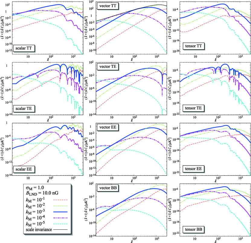
Figure 1: CMB spectra from the LND-PMF at $\sigma_{\mathrm{M}}=1.0$ and $B_{\mathrm{LND}}=$10nG. TT, EE, BB and TE in each panel indicate the temperature auto-correlation, the E-mode auto-correlation, the B-mode auto-correlation and the temperature E-mode cross correlation, respectively Curves in all panels are theoretical lines as indicated in the legend box at the left bottom. Curves of all TE modes are plotted in the absolute value.

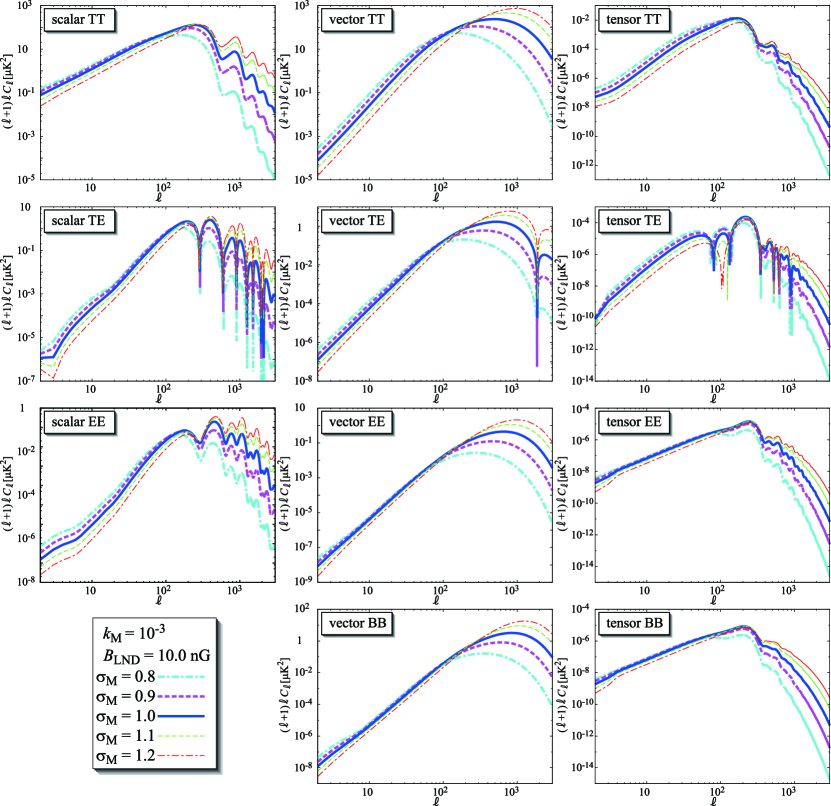
Figure 2: CMB spectra from the LND-PMF at $k_{\mathrm{M}}=10^{-3}$ and $B_{\mathrm{LND}}=$10nG. Curves in all panels are theoretical lines as indicated in the legend box at the left bottom. Curves of all TE modes are plotted in the absolute value.

Figures 1 and 2 show the four modes of the CMB (TT, EE, BB, and TE modes) from the LND-PMF. Since qualitative features of the scalar, vector, and tensor modes on the CMB are almost the same as previous studies Kojima et al. (2008); Kahniashvili et al. (2008); Yamazaki et al. (2009); Yamazaki et al. (2010b), in this article, we will briefly explain these features of the CMB with the PMF as follows.

In general, the vector mode dominates all the temperature and polarization auto- and cross-correlation anisotropies at $\ell\gtrsim 500$, while the scalar mode dominates at smaller $\ell$, except for the BB mode. For BB mode of the CMB, the vector mode dominates the power spectrum for all $\ell$.

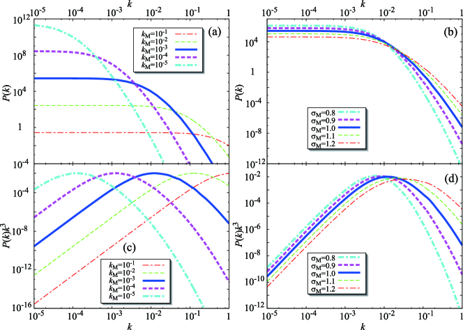
Figure 3: Power spectrum of the energy density of the PMF. Panels (a) and (c) on this figure are for the fixed $\sigma_{\mathrm{M}}$ value at $\sigma_{\mathrm{M}}=1.0$, and panels (b) and (d) are for the fixed $k_{\mathrm{M}}$ value at $k_{\mathrm{M}}=10^{-3}$. Curves in different colors in all panels correspond to the different PMF parameters as indicated in the legend box in the figure. Note that from Eqs.(LABEL:p:se)-(LABEL:p:t) we see that the other spectra, such as magnetic tension, anisotropic stress and so on, have very similar shape to that of the energy density so we only show the spectrum of the energy density in the figure.

To understand the feature of temperature fluctuations and polarization anisotropies of the CMB from the LND-PMF in Fig.1, we shall go back to the definitions $\mathrm{Eqs.}(\ref{eq:power_lg}),(\ref{p:se})-(\ref{p:t})$ and show Fig.3 which depicts $P(k)$ and $P(k)\times k^{3}$. From the definition of Eq.(14), we can understand that the peak amplitudes of the LND-PMF power spectra of each $k_{\mathrm{M}}$ for the CMB spectra are along the scale invariant amplitude [see panel (c) of Fig.3]. Therefore, the superposition of the spectra of CMB anisotropy from different $k_{\mathrm{M}}$ corresponds to the spectra from the scale invariant magnetic fields. Indeed in the top-center panel of Fig.1, we find that the points of the CMB power spectra on the same $\sigma_{\mathrm{M}}$, which are corresponding to the peak of the $P(k)\times k^{3}$, are distributed along the scale invariant curve. We should note that the peak position of the LND-PMF source $P(k)\times k^{3}$ is different from one of the eventual power spectra of the CMB, because the final spectrum should be obtained by multiplying the LND-PMF power spectrum by the linear transfer functions which include various physical effects including the PMF.

Considering the mathematical definition of Eq.(14) as mentioned above, the peak scale of the LND-PMF power spectrum is determined by $k_{\mathrm{M}}$. We find, however, that the peak positions of the CMB spectra from the PMF power spectrum are characterized not only by $k_{\mathrm{M}}$ but also by $\sigma_{\mathrm{M}}$. The reason is as follows. The LND-PMF power spectrum $P(k)$ becomes more broad with increasing $\sigma_{\mathrm{M}}$ as shown in panel (b) of Fig.3. The amplitudes of the CMB power spectra are determined by $k^{3}P(k)$ which is plotted in the panel (d) of Fig.3. The peak position in terms of the combination $k^{3}P(k)$ is affected also by $\sigma_{\mathrm{M}}$, and hence the positions of the peaks in CMB power spectra are also affected by $\sigma_{\mathrm{M}}$.

Considering the scale dependencies of the scalar and vector modes Paoletti et al. (2009); Finelli et al. (2008); Shaw and Lewis (2010); Yamazaki et al. (2010a), in the case of the smaller $k_{\mathrm{M}}$ and/or smaller $\sigma_{\mathrm{M}}$ the scalar mode determines the maximum amplitude of the power spectra of the CMB and dominates the power spectra at smaller angular moments $\ell<1000$. Meanwhile, in the case of the larger $k_{\mathrm{M}}$ and/or larger $\sigma_{\mathrm{M}}$, the vector mode determines the maximum amplitude and dominates at larger $\ell$. In this case, since the peak of the total power spectrum from the LND-PMF lies among 1000 $<\ell<$ 2000 (e.g., for $\sigma_{\mathrm{M}}=1.0$, $k_{\mathrm{[LND]}}\sim 1.0^{-2}$, see Fig.4), we can expect that the observation data of the CMB among 1000 $<\ell<$ 2000 better constrain LND-PMF parameters.

IV.2 How are LND-PMF parameters constrained by the CMB?

In the above sections, we have explained the behaviors of the power spectrum of the PMF from LND distributions and the effects on the CMB. In this subsection, considering these features, we discuss how LND-PMF parameters, $k_{\mathrm{M}}$, $\sigma_{\mathrm{M}}$ and $B_{\mathrm{LND}}$ are constrained by the CMB observations. As mentioned in the above sections, the peak positions of the spectra of PMF electromagnetic tensors mainly depend on the characteristic wavenumber $k_{\mathrm{M}}$ and $\sigma_{\mathrm{M}}$, the amplitudes mainly depend on $k_{\mathrm{M}}$ and $B_{\mathrm{LND}}$, and the features the peak width and the damping scale depend on the $\sigma_{\mathrm{M}}$. Figures 4 and 5 show the CMB (TT, EE, BB and TE) angular power spectra from primary (standard adiabatic mode without the PMF) and from the LND-PMF along with observations (WMAP Larson et al. (2011), ACBAR Reichardt et al. (2009), CBI Sievers et al. (2007) and QUaD Brown et al. (2009)). Considering the above mentioned facts, if $k_{\mathrm{M}}$ or $\sigma_{\mathrm{M}}$ is larger, the PMF amplitude is constrained by the CMB observation data at smaller scales. On the other hand, if $k_{\mathrm{M}}$ or $\sigma_{\mathrm{M}}$ is smaller, the PMF amplitude is constrained by the CMB at larger scales. The strength of the PMF $B_{\mathrm{LND}}$ monotonically increases or decreases the amplitude of CMB power spectra from the LND-PMF. These features may suggest a significant anticorrelation between the characteristic wavenumber $k_{\mathrm{M}}$ and the variance $\sigma_{\mathrm{M}}$. Meanwhile, the slopes of the spectrum at small scale are mainly characterized by the variance $\sigma_{\mathrm{M}}$.

To research how the strength of the LND-PMF is constrained by the CMB observations on each characteristic scale $k_{\mathrm{M}}$, we perform a Markov chain Monte Carlo analysis with the CMB observations and obtain the constraint on the $B_{\mathrm{LND}}$-$k_{\mathrm{M}}$ plane. Since our purpose is qualitatively understanding how the primordial magnetic fields are constrained scale by scale the variance parameter of the LND-PMF is fixed at $\sigma_{\mathrm{M}}=1$ for simplicity and we also fix the cosmological parameters to those of the best-fit flat $\Lambda$CDM model as given in the WMAP 7yr analysis Larson et al. (2011).

Figure 6 shows the constrained strengths of the LND-PMF from the CMB observations (WMAP 7th, ACBAR, CBI, Boomerang, and QuaD) for each scale. From this figure, the LND-PMFs at $10^{-3}$ Mpc $\leq~{}k~{}\leq~{}10^{-2}$ Mpc are most tightly constrained.

V Summary

It is natural to assume that the power spectrum of the PMF from inflation is the power law. However, when we consider PMF generated by causal mechanisms, it would be appropriate to assume a spectrum with a characteristic scale. In this paper, we assumed the log-normal distribution as the PMF spectrum and studied the effects of the PMFs on the temperature and polarization anisotropies of the CMB. We have revealed the features of the LND-PMF effects on the CMB as follows: (1) For larger $k_{\mathrm{M}}$ and/or $\sigma_{\mathrm{M}}$, the CMB spectra of TT, TE and EE from the LND-PMF are dominated by the vector mode. Meanwhile, in the opposite case, these spectra are dominated by the scalar mode. (2) The CMB spectrum of the BB mode for all scales and other modes for smaller scales is dominated by the vector modes. Because three parameters which characterize the LND-PMF affect the CMB power spectra differently at small and large scales we expect that tight constraints can be placed on these parameters without degeneracy. We found that the LND-PMF which generates CMB anisotropies among 1000 $<\ell<$ 2000 is most effectively constrained by the current CMB data sets. For example, $B_{\mathrm{LND}}$ for $10^{-3}\mathrm{Mpc}^{-1}~{}\leq~{}k/h~{}\leq 10^{-2}\mathrm{Mpc}^{-1}$ and $\sigma_{\mathrm{M}}=1.0$ is limited most strongly as shown in Fig.6. In the near future, the tighter constraints on $B_{\mathrm{LND}}$ at $k_{\mathrm{M}}/h>10^{-2}$Mpc^-1 will be expected from the observations, such as the Planck, QUIET, and PolarBear missions.

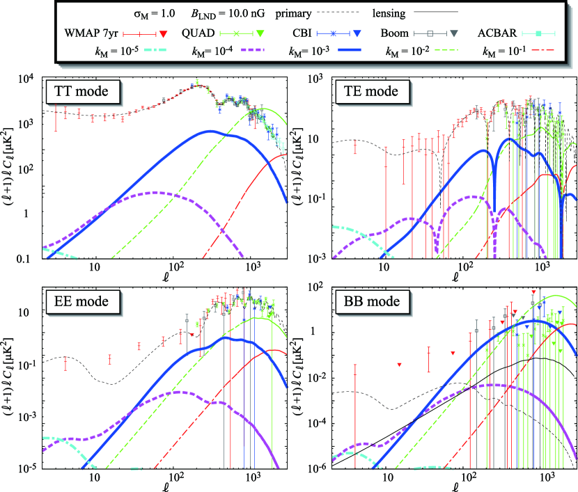
Figure 4: Comparison of total CMB spectra from the LND-PMF at $\sigma_{\mathrm{M}}=1.0$ and $B_{\mathrm{LND}}=$10nG with the best-fitting CMB power spectra without the LND-PMF (dashed line). Curves in all panels are the theoretical lines as indicated in the legend box on the figure. Curves of the TE mode are plotted in the absolute value.

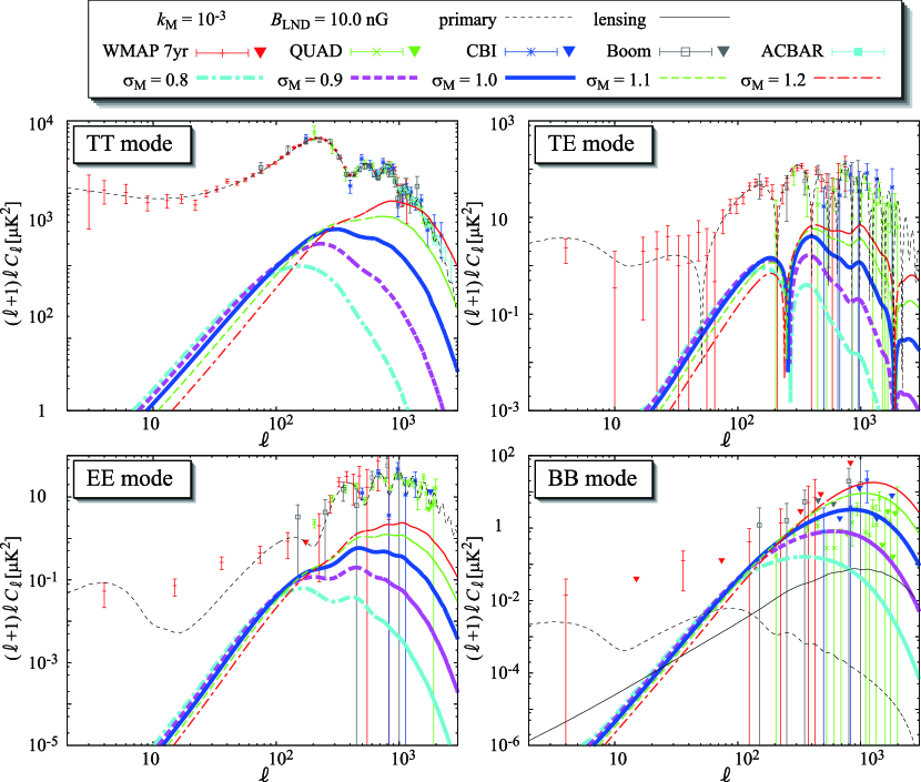
Figure 5: Comparison of total CMB spectra from the LND-PMF at $k_{\mathrm{M}}=10^{-3}$ and $B_{\mathrm{LND}}=$10nG with the best-fitting CMB power spectra without the LND-PMF (dashed line). Curves in all panels are the theoretical lines as indicated in the legend box on the figure. Curves of the TE mode are plotted in the absolute value.

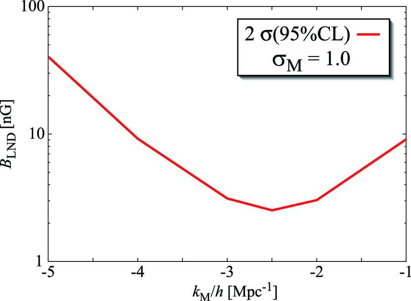
Figure 6: Constraint on the strengths of LND-PMF for $10^{-5}<k_{\mathrm{M}}<10^{-1}$. The bold curve is the 2 $\sigma$ upper limits of $B_{\mathrm{LND}}$ [nG]. We fix the standard cosmological parameters and use the best-fitted value from WMAP 7th + tensor modeLarson et al. (2011).

References

• Subramanian and Barrow (1998) K. Subramanian and J. D. Barrow, Phys. Rev. Lett. 81, 3575 (1998).
• Mack et al. (2002) A. Mack, T. Kahniashvili, and A. Kosowsky, Phys. Rev. D 65, 123004 (2002).
• Subramanian and Barrow (2002) K. Subramanian and J. D. Barrow, Mon. Not. Roy. Astron. Soc. 335, L57 (2002).
• Lewis (2004) A. Lewis, Phys. Rev. D 70, 043011 (2004).
• Yamazaki et al. (2005a) D. G. Yamazaki, K. Ichiki, and T. Kajino, Astrophys. J. 625, L1 (2005a).
• Kahniashvili and Ratra (2005) T. Kahniashvili and B. Ratra, Phys. Rev. D 71, 103006 (2005).
• Challinor (2004) A. Challinor, Lect. Notes Phys. 653, 71 (2004).
• Dolgov (2005) A. D. Dolgov (2005), eprint astro-ph/0503447.
• Gopal and Sethi (2005) R. Gopal and S. K. Sethi, Phys. Rev. D 72, 103003 (2005).
• Yamazaki et al. (2005b) D. G. Yamazaki, K. Ichiki, and T. Kajino, Nuclear Physics A 758, 791 (2005b).
• Kahniashvili and Ratra (2007) T. Kahniashvili and B. Ratra, Phys. Rev. D75, 023002 (2007).
• Yamazaki et al. (2006a) D. G. Yamazaki, K. Ichiki, K. I. Umezu, and H. Hanayama, Phys. Rev. D 74, 123518 (2006a).
• Yamazaki et al. (2006b) D. G. Yamazaki, K. Ichiki, T. Kajino, and G. J. Mathews, Astrophys. J. 646, 719 (2006b).
• Yamazaki et al. (2006c) D. G. Yamazaki, K. Ichiki, T. Kajino, and G. J. Mathews, PoS(NIC-IX). p. 194 (2006c).
• Giovannini (2006a) M. Giovannini, Phys. Rev. D 74, 063002 (2006a).
• Yamazaki et al. (2008) D. G. Yamazaki, K. Ichiki, T. Kajino, and G. J. Mathews, Phys. Rev. D 77, 043005 (2008).
• Paoletti et al. (2009) D. Paoletti, F. Finelli, and F. Paci, Mon. Not. Roy. Astron. Soc. 396, 523 (2009).
• Finelli et al. (2008) F. Finelli, F. Paci, and D. Paoletti, Phys. Rev. D78, 023510 (2008), eprint 0803.1246.
• Yamazaki et al. (2008) D. G. Yamazaki, K. Ichiki, T. Kajino, and G. J. Mathews, Phys. Rev. D 78, 123001 (2008).
• Yamazaki et al. (2008) D. G. Yamazaki, K. Ichiki, T. Kajino, and G. J. Mathews, PoS(NIC-X). p. 239 (2008).
• Sethi et al. (2008) S. K. Sethi, B. B. Nath, and K. Subramanian, Mon. Not. Roy. Astron. Soc. 387, 1589 (2008).
• Kojima et al. (2008) K. Kojima, K. Ichiki, D. G. Yamazaki, T. Kajino, and G. J. Mathews, Phys. Rev. D78, 045010 (2008).
• Kahniashvili et al. (2008) T. Kahniashvili, G. Lavrelashvili, and B. Ratra, Phys. Rev. D78, 063012 (2008).
• Giovannini and Kunze (2008) M. Giovannini and K. E. Kunze, Phys. Rev. D78, 023010 (2008), eprint 0804.3380.
• Yamazaki et al. (2009) D. G. Yamazaki, K. Ichiki, T. Kajino, and G. J. Mathews, submitted p.   (2009).
• Shaw and Lewis (2010) J. R. Shaw and A. Lewis, Phys. Rev. D 81, 043517 (2010).
• Yamazaki et al. (2010a) D. G. Yamazaki, K. Ichiki, T. Kajino, and G. J. Mathews, Phys. Rev. D 81, 023008 (2010a).
• Yamazaki et al. (2010b) D. G. Yamazaki, K. Ichiki, T. Kajino, and G. J. Mathews, Phys. Rev. D 81, 103519 (2010b).
• Yamazaki et al. (2010c) D. G. Yamazaki, K. Ichiki, T. Kajino, and G. J. Mathews, Adv. Astron. 2010, 586590 (2010c).
• Turner and Widrow (1988) M. S. Turner and L. M. Widrow, Phys. Rev. D 37, 2743 (1988).
• Ratra (1992) B. Ratra, Astrophys. J. 391, L1 (1992).
• Bamba and Yokoyama (2004) K. Bamba and J. Yokoyama, Phys. Rev. D 70, 083508 (2004).
• Bamba and Yokoyama (2004) K. Bamba and J. Yokoyama, Phys. Rev. D 69, 043507 (2004).
• Bamba and Sasaki (2007) K. Bamba and M. Sasaki, J. Cosmol. Astropart. Phys. 02, 30 (2007).
• Takahashi et al. (2005) K. Takahashi, K. Ichiki, H. Ohno, and H. Hanayama, Phys. Rev. Lett. 95, 121301 (2005).
• Ichiki et al. (2006) K. Ichiki, K. Takahashi, H. Ohno, H. Hanayama, and N. Sugiyama, Science 311, 827 (2006).
• Hanayama et al. (2005) H. Hanayama et al., Astrophys. J. 633, 941 (2005).
• Fujita and Kato (2005) Y. Fujita and T. N. Kato, Mon. Not. R. Astron. Soc. 364, 247 (2005).
• Christensson et al. (2001) M. Christensson, M. Hindmarsh, and A. Brandenburg, Phys. Rev. E 64, 056405 (2001).
• Banerjee and Jedamzik (2004) R. Banerjee and K. Jedamzik, Phys. Rev. D 70, 123003 (2004).
• Durrer et al. (2000) R. Durrer, P. G. Ferreira, and T. Kahniashvili, Phys. Rev. D 61, 043001 (2000).
• Kahniashvili et al. (2010) T. Kahniashvili, A. Brandenburg, A. G. Tevzadze, and B. Ratra, Phys. Rev. D 81, 123002 (2010).
• Ma and Bertschinger (1995) C.-P. Ma and E. Bertschinger, Astrophys. J. 455, 7 (1995).
• Hu and White (1997) W. Hu and M. J. White, Phys. Rev. D 56, 596 (1997).
• Padmanabhan (1993) T. Padmanabhan, Structure formation in the universe (Cambridge University Press, 1993).
• Hu et al. (1998) W. Hu, U. Seljak, M. J. White, and M. Zaldarriaga, Phys. Rev. D 57, 3290 (1998).
• Dodelson (2003) S. Dodelson, Modern Cosmology (Academic Press, 2003).
• Giovannini (2006b) M. Giovannini, Class. Quant. Grav. 23, 4991 (2006b).
• Cai et al. (2010) R. Cai, B. Hu, and H. Zhang, JCAP 8, 25 (2010).
• Lewis et al. (2000) A. Lewis, A. Challinor, and A. Lasenby, Astrophys. J. 538, 473 (2000).
• Larson et al. (2011) D. Larson, J. Dunkley, G. Hinshaw, E. Komatsu, M. R. Nolta, C. L. Bennett, B. Gold, M. Halpern, R. S. Hill, N. Jarosik, et al., Astrophys. J.S. 192, 16 (2011).
• Reichardt et al. (2009) C. L. Reichardt, P. A. R. Ade, J. J. Bock, J. R. Bond, J. A. Brevik, C. R. Contaldi, M. D. Daub, J. T. Dempsey, J. H. Goldstein, W. L. Holzapfel, et al., Astrophys. J. 694, 1200 (2009).
• Sievers et al. (2007) J. L. Sievers, C. Achermann, J. R. Bond, L. Bronfman, R. Bustos, C. R. Contaldi, C. Dickinson, P. G. Ferreira, M. E. Jones, A. M. Lewis, et al., Astrophys. J. 660, 976 (2007).
• Brown et al. (2009) M. L. Brown, P. Ade, J. Bock, M. Bowden, G. Cahill, P. G. Castro, S. Church, T. Culverhouse, R. B. Friedman, K. Ganga, et al., Astrophys. J. 705, 978 (2009).