Entropy of stochastic blockmodel ensembles

Abstract

Stochastic blockmodels are generative network models where the vertices are separated into discrete groups, and the probability of an edge existing between two vertices is determined solely by their group membership. In this paper, we derive expressions for the entropy of stochastic blockmodel ensembles. We consider several ensemble variants, including the traditional model as well as the newly introduced degree-corrected version [Karrer et al. Phys. Rev. E 83, 016107 (2011)], which imposes a degree sequence on the vertices, in addition to the block structure. The imposed degree sequence is implemented both as “soft” constraints, where only the expected degrees are imposed, and as “hard” constraints, where they are required to be the same on all samples of the ensemble. We also consider generalizations to multigraphs and directed graphs. We illustrate one of many applications of this measure by directly deriving a log-likelihood function from the entropy expression, and using it to infer latent block structure in observed data. Due to the general nature of the ensembles considered, the method works well for ensembles with intrinsic degree correlations (i.e. with entropic origin) as well as extrinsic degree correlations, which go beyond the block structure.

I Introduction

Stochastic blockmodels Holland et al. (1983); Fienberg et al. (1985); Faust and Wasserman (1992); Anderson et al. (1992) are random graph ensembles, in which vertices are separated into discrete groups (or “blocks”), and the probability of an edge existing between two vertices is determined according to their group membership. This class of model (together with many variants which incorporate several other details Doreian et al. (2004); Brandes et al. (2010)) has been used extensively in the social sciences, where the blocks usually represents the roles played by different social agents. In this context, it has been used mainly as a tool to infer latent structure in empirical data. More recently, it has been applied as an alternative to the more specific task of community detection Fortunato (2010), which focus solely on densely connected communities of vertices Newman and Leicht (2007); Reichardt and White (2007); Bickel and Chen (2009); Guimerà and Sales-Pardo (2009); Karrer and Newman (2011); Ball et al. (2011); Reichardt et al. (2011); Decelle et al. (2011). In addition to its usefulness in this context, stochastic blockmodels serve as a general framework which has many potential applications, such as the parametrization of network topologies on which dynamical processes can occur Peixoto (2012a, b), and in the modelling of adaptive networks, where the topology itself can vary according to dynamical rules Gross and Blasius (2008).

The standard stochastic blockmodel formulation Holland et al. (1983) assumes that all vertices belonging to the same block are statistically indistinguishable, which means that they all have the same expected degree. This restriction is not very attractive for a general model, since many observed networks show an extreme variation of degrees, even between vertices perceived to be of the same block (or “community”). Recently, this class of model has been augmented by the introduction of the “degree-corrected” variant Karrer and Newman (2011), which incorporates such degree variation, and was shown to be a much better model for many empirical networks. With this modification, the stochastic blockmodel becomes more appealing, since (except for the degrees) it only discards local scale properties of the network topology (such as clustering, motifs, etc. Newman (2010)), but can represent well arbitrary global or mesoscale properties, such as assortativity/dissortativity Newman (2003a), community structure Girvan and Newman (2002); Fortunato (2010), bipartite and multipartite adjacency, and many others.

In this work, we focus on the microcanonical entropy Bianconi (2008); Anand and Bianconi (2009); Bianconi (2009); Anand and Bianconi (2010) of stochastic blockmodel ensembles, defined as $\mathcal{S}=\ln\Omega$, where $\Omega$ is the number of graphs in the ensemble. This quantity has the traditional interpretation of measuring the degree of “order” of a given ensemble, which is more disordered (i.e. random) if the entropy is larger. It is also a thermodynamic potential, which, in conjunction with other appropriate quantities such as energy — representing different sorts of interactions, such as homophily in social systems Castellano et al. (2009) or robustness in biological dynamical models Peixoto (2012a) — can be used to describe the equilibrium properties of evolved network systems Strauss (1986); Burda et al. (2001); Park and Newman (2004a, b); Palla et al. (2004); Burda et al. (2004); Biely and Thurner (2006); Fronczak et al. (2006, 2007); Jeong et al. (2007); Foster et al. (2010); Peixoto (2012a).

From the entropy $\mathcal{S}$ one can directly derive the log-likelihood function $\mathcal{L}=\ln\mathcal{P}$, where $\mathcal{P}$ is the probability of observing a given network realization, which is used often in the blockmodel literature. Assuming that each graph in the ensemble is realized with the same probability, $\mathcal{P}=1/\Omega$, we have simply that $\mathcal{L}=-\mathcal{S}$. The log-likelihood can be used to infer the most likely block structure which matches a given network data, and thus plays a central role in the context of blockmodel detection. However, the expressions for the log-likelihood $\mathcal{L}$, as they are often derived in the stochastic blockmodel literature, do not allow one to directly obtain the entropy, either because the they are expressed in non-closed form Holland et al. (1983); Fienberg et al. (1985); Faust and Wasserman (1992); Anderson et al. (1992); Nowicki and Snijders (2001); Reichardt et al. (2011); Ball et al. (2011), or because they only contain terms which depend on a posteriori partition of a sample network, with the remaining terms neglected Bickel and Chen (2009); Karrer and Newman (2011); Ball et al. (2011).

In this work, we derive expressions for the entropy of elementary variations of the blockmodel ensembles. The choice of microcanonical ensembles permits the use of straightforward combinatorics, which simplify the analysis. We consider both the traditional and degree-corrected variants of the model, as well as their implementations as ensembles of multigraphs (with parallel edges and self-loops allowed) and simple graphs (no parallel edges or self-loops allowed). The degree-corrected variants considered here represent a generalization of the original definition Karrer and Newman (2011), since arbitrary nearest-neighbours degree correlations are also allowed. For the degree-corrected variants, we consider the imposed degree sequence on the vertices both as “soft” and “hard” constraints: When the degree constraints are “soft”, it is assumed that the imposed degree on each vertex is only an average over the ensemble, and their values over sampled realizations are allowed to fluctuate. With “hard” constraints, on the other hand, it is imposed that the degree sequence is always the same on all samples of the ensemble. We also consider the directed versions of all ensembles. These represent further refinements of the original definition Karrer and Newman (2011), which considered only undirected graphs with “soft” degree constraints.

The entropy expressions derived represent generalizations of several expressions found in the literature for the case without block structure Bender (1974); Bender and Butler (1978); Wormald (1999); Bianconi (2009), which are easily recovered by setting the number of blocks to one.

As a direct application of the derived entropy functions, we use them to define a log-likelihood function $\mathcal{L}$, which can be used to detect the most likely blockmodel partition which fits a given network data. We show that these estimators work very well to detect block structures in networks where there are intrinsic (as in the case of simple graphs with broad degree distributions) or extrinsic degree correlations. In particular, the expressions derived in this work perform better for networks with broad degree distributions than the sparse approximation derived in Karrer and Newman (2011), which may result in suboptimal partitions.

This paper is divided as follows. In Sec. II we define the traditional and degree-corrected stochastic blockmodel ensembles. In Secs. III to V we systematically derive analytical expressions for the most fundamental ensemble variants, including simple graphs (Sec. III) and multigraphs (Sec. IV), both the traditional and (soft) degree-corrected versions, as well as the undirected and directed cases. In Sec. V we obtain the entropy for the degree-corrected ensembles with hard degree constraints, for the same variants described in the other sections. In Sec. VI we apply the derived entropy expression for the soft degree-corrected ensemble to the problem of blockmodel detection, by using it as a log-likelihood function. [Readers more interested in the application to blockmodel detection can read Secs. II to III.2, and then move directly to Sec. VI.] We finalize in Sec. VII with a conclusion.

II Traditional and degree-corrected blockmodels

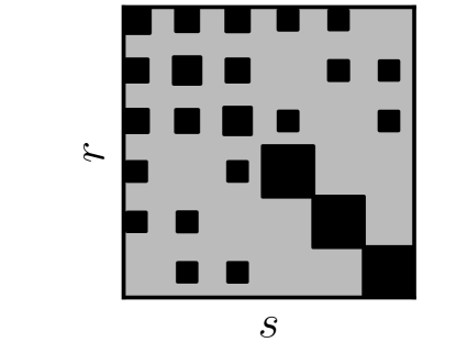
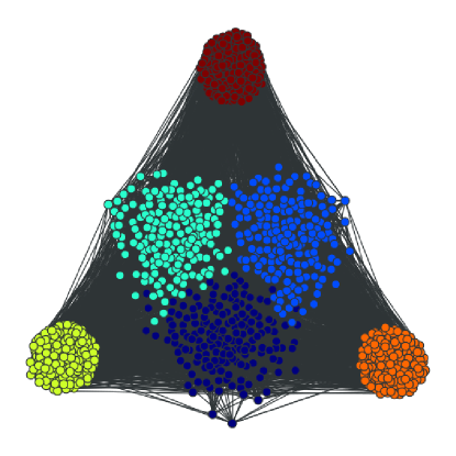
The traditional blockmodel ensemble is parametrized as follows: There are $N$ vertices, partitioned into $B$ blocks, and $n_{r}$ is number of vertices in block $r\in[0,B-1]$. The matrix $e_{rs}$ specifies the number of edges between blocks $r$ and $s$, which are randomly placed. As matter of convenience, the diagonal elements $e_{rr}$ are defined as twice the number of edges internal to the block $r$ (or equivalently, the number of “half-edges”). An example of a specific choice of parameters can be seen in Fig. 1.

This is a “microcanonical” formulation of the usual “canonical” form which specifies instead the probability $w_{rs}$ of an edge occurring between two vertices belonging to blocks $r$ and $s$, so that the expected number of edges $e_{rs}=Ew_{rs}$ is allowed to fluctuate, where $E$ is the total number of edges. If the nonzero values of $e_{rs}$ are sufficiently large, these two ensembles become equivalent, since in this case fluctuations around the mean value can be neglected.

Figure 1: (Color online) Example of a traditional stochastic blockmodel with six blocks of equal size, and matrix $e_{rs}$ given on the left (each square is a matrix element, and its size corresponds to its magnitude). On the right is a sample of this ensemble with $10^{3}$ vertices.

The degree-corrected variant Karrer and Newman (2011) further imposes a degree sequence $\{k_{i}\}$ on each vertex $i\in[0,N-1]$ of the network, which must be obeyed in addition to the block structure specified by $n_{r}$ and $e_{rs}$. This restriction may be imposed in two different ways. The first approach assumes these constraints are “soft”, and each individual degree $k_{i}$ represents only the average value of the degree of vertex $i$ over all samples of the ensemble Chung and Lu (2002a, b) (this is the original ensemble defined in Karrer and Newman (2011)). Here, we will also consider a second approach which assumes the degree constraints are “hard”, and the imposed degree sequence must be exactly the same in all samples of the ensemble. We will obtain the entropy for both these ensembles in the following.

III Simple graph ensembles

III.1 Standard stochastic blockmodel

In simple graphs there can be at most only one edge between two vertices. Therefore, we can enumerate the total number of different edge choices between blocks $r$ and $s$ as,

$$\Omega_{rs}={n_{r}n_{s}\choose e_{rs}},\qquad\Omega_{rr}={{n_{r}\choose 2}\choose\frac{e_{rr}}{2}},$$ (1)

which leads to the total number of graphs,

$$\Omega=\prod_{r\geq s}\Omega_{rs}.$$ (2)

The entropy is obtained by $\mathcal{S}_{g}=\ln\Omega$. Considering the values of $n_{r}$ large enough so that Stirling’s approximation can be used, expressed as $\ln{N\choose m}\cong NH(m/N)$, where $H(x)$ is the binary entropy function,

$$H(x) =-x\ln x-(1-x)\ln(1-x)$$ (3)

$$=-x\ln x+x-\sum_{l=1}^{\infty}\frac{x^{l+1}}{l(l+1)},$$ (4)

we obtain the compact expression,

$$\mathcal{S}_{g}=\frac{1}{2}\sum_{rs}n_{r}n_{s}H\left(\frac{e_{rs}}{n_{r}n_{s}}\right).$$ (5)

Eq. 5 has been derived by other means in Bickel and Chen (2009) (expressed as a log-likelihood function), for the canonical variant of the ensemble. Making use of the series expansion given by Eq. 4, the entropy can be written alternatively as

$$\mathcal{S}_{g}=E-\frac{1}{2}\sum_{rs}e_{rs}\ln\left(\frac{e_{rs}}{n_{r}n_{s}}\right)\\ -\frac{1}{2}\sum_{rs}n_{r}n_{s}\sum_{l=1}^{\infty}\frac{1}{l(l+1)}\left(\frac{e_{rs}}{n_{r}n_{s}}\right)^{l+1},$$ (6)

where $E=\sum_{rs}e_{rs}/2$ is the total number of edges in the network. The terms in the last sum in the previous expression are of the order $O(e^{2}_{rs}/n_{r}n_{s})$. This number is typically of the order $\sim{\left<k\right>}^{2}$, where ${\left<k\right>}$ is the average degree of the network. Since the other terms of the expression are of order $\sim{\left<k\right>}{N}$, and one often has that ${\left<k\right>}\ll N$, the last term can be dropped, which leads to,

$$\mathcal{S}_{g}\cong E-\frac{1}{2}\sum_{rs}e_{rs}\ln\left(\frac{e_{rs}}{n_{r}n_{s}}\right).$$ (7)

The last term of Eq. 7 is compatible with the equivalent expression for the log-likelihood derived in Karrer and Newman (2011). We note that while this limit can be assumed in many practical scenarios, one can also easily imagine ensembles which are “globally sparse” (i.e. ${\left<k\right>}\ll N$), but “locally dense”, with ${\left<k\right>}_{r}=e_{r}/n_{r}\sim n_{s}$, for any two blocks $r$, $s$ (with $e_{r}=\sum_{s}e_{rs}$ being the total number of half-edges adjacent to block $r$). In such scenarios Eq. 7 will neglect potentially important contributions to the entropy, and therefore Eqs. 5 or 6 should be used instead.

As shown in Karrer and Newman (2011), the second term of Eq. 7 can be slightly rewritten as the Kullback-Leibler divergence Cover and Thomas (1991) between the actual and expected distributions of block assignments at the opposing ends of randomly chosen edges, where the expected distribution takes into account only the size of each block. This can be interpreted as the amount of additional information required to encode a given block partition, if one assumes a priori that the amount of edges incident to each block is proportional to its size.

III.1.1 Directed graphs

The ensemble of directed blockmodels can be analysed in an analogous fashion. The only differences is that for the directed version, the matrix $e_{rs}$ can be asymmetric, and one needs to differentiate between the number of edges leaving block $r$, $e^{+}_{r}=\sum_{s}e_{rs}$, and the number of edges arriving, $e^{-}_{r}=\sum_{s}e_{sr}$. The number of edge choices $\Omega_{rs}$ is given exactly as in Eq. 1, the only difference being that one no longer needs to differentiate the diagonal term, which in this case becomes $\Omega_{rr}\equiv\Omega_{rs}|_{s=r}$. Since the matrix $e_{rs}$ is in general asymmetric, the total number of graphs becomes the product over all directed $r,s$ pairs,

$$\Omega=\prod_{rs}\Omega_{rs}.$$ (8)

Therefore the entropy becomes simply,

$$\mathcal{S}_{g}=\sum_{rs}n_{r}n_{s}H\left(\frac{e_{rs}}{n_{r}n_{s}}\right),$$ (9)

which is identical to Eq. 5, except for a factor $1/2$ (Note that for directed graphs we define $e_{rr}$ as the number of edges internal to block $r$, not twice this value as in the undirected case). Naturally, the same alternative expression as in Eq. 6 can be written, as well as the same approximation as in Eq. 7, which will be identical except for a factor $1/2$.

III.2 Degree-corrected ensembles with “soft” constraints

Following Karrer and Newman (2011), we introduce degree variability to the blockmodel ensemble defined previously, by imposing an expected degree sequence $\{\kappa_{i}\}$ on all vertices of the graph, in addition to their block membership. Thus each individual $\kappa_{i}$ represents only the average value of the degree of vertex $i$ over all samples of the ensemble. Such “soft” degree constraints are relatively easy to implement, since one needs only to extend the non degree-corrected version, simply by artificially separating vertices with given imposed expected degrees into different degree blocks. Thus, each existent block is labeled by a pair $(r,\kappa)$, where the first value is the block label itself, and the second is the expected degree label. In order for the label $(r,\kappa)$ to be meaningful, we need to have intrinsically that $e_{(r,\kappa)}=\sum_{s\kappa^{\prime}}e_{(r,\kappa),(s,\kappa^{\prime})}=\kappa n_{(r,\kappa)}$, such that the average degree of vertices in block $(r,\kappa)$ is exactly $\kappa$. This results in an ensemble with $KB$ blocks, where $K$ is the total number of different expected degrees, $n_{(r,\kappa)}$ is the number of vertices in block $(r,\kappa)$, and $e_{(r,\kappa),(s,\kappa^{\prime})}$ is number of edges between $(r,\kappa)$ and $(s,\kappa^{\prime})$. Inserting this block structure into Eq. 5, one obtains

$$\mathcal{S}_{gs}=\frac{1}{2}\sum_{\begin{subarray}{c}r\kappa s\kappa^{\prime}\end{subarray}}n_{(r,\kappa)}n_{(s,\kappa^{\prime})}H\left(\frac{e_{(r,\kappa),(s,\kappa^{\prime})}}{n_{(r,\kappa)}n_{(s,\kappa^{\prime})}}\right).$$ (10)

This ensemble accommodates not only blockmodels with arbitrary (expected) degree sequences, but also with arbitrary degree correlations, since it is defined as a function of the full matrix $e_{(r,\kappa),(s,\kappa^{\prime})}$ (It is therefore a generalization of the ensemble defined in Karrer and Newman (2011)). However, it is often more useful to consider the less-constrained ensemble where one restricts only the total number of edges between blocks, irrespective of their expected degrees,

$$e_{rs}=\sum_{\kappa\kappa^{\prime}}e_{(r,\kappa),(s,\kappa^{\prime})}.$$ (11)

This can be obtained by maximizing the entropy $\mathcal{S}_{gs}$, subject to this constraint. Carrying out this maximization, one arrives at the following nonlinear system,

$$e_{(r,\kappa),(s,\kappa^{\prime})} =\frac{n_{(r,\kappa)}n_{(s,\kappa^{\prime})}}{\exp(\lambda_{rs}+\mu_{r\kappa}+\mu_{s\kappa^{\prime}})+1}$$ (12)

$$e_{rs} =\sum_{\kappa\kappa^{\prime}}e_{(r,\kappa),(s,\kappa^{\prime})}$$ (13)

$$\kappa n_{(r,\kappa)} =\sum_{s\kappa^{\prime}}e_{(r,\kappa),(s,\kappa^{\prime})}$$ (14)

which must be solved for $\{e_{(r,\kappa),(s,\kappa^{\prime})},\lambda_{rs},\mu_{r\kappa}\}$, where $\{\lambda_{rs}\}$ and $\{\mu_{r\kappa}\}$ are Lagrange multipliers which impose the necessary constraints, described by Eqs. 13 and 14, respectively. Unfortunately, this system admits no general closed-form solution. However, if one makes the assumption that $\exp(\lambda_{rs}+\mu_{r\kappa}+\mu_{s\kappa^{\prime}})\gg 1$, one obtains the approximate solution,

$$e_{(r,\kappa),(s,\kappa^{\prime})}\cong\frac{e_{rs}}{e_{r}e_{s}}n_{(r,\kappa)}n_{(s,\kappa^{\prime})}\kappa\kappa^{\prime}.$$ (15)

This is often called the “sparse” or “classical” limit Park and Newman (2004a), and corresponds to the limit where intrinsic degree correlations between any two blocks $r$ and $s$ can be neglected . Eq. 15 is intuitively what one expects for uncorrelated degree-corrected blockmodels: The number of edges between $(r,\kappa)$ and $(s,\kappa^{\prime})$ is proportional to the number of edges between the two blocks $e_{rs}$ and the degree values themselves, $\kappa\kappa^{\prime}$. Including this in Eq. 10, and using Eq. 4 one obtains,

$$\mathcal{S}_{gsu}\cong E-\sum_{\kappa}N_{\kappa}\kappa\ln\kappa-\frac{1}{2}\sum_{rs}e_{rs}\ln\left(\frac{e_{rs}}{e_{r}e_{s}}\right)\\ -\frac{1}{2}\sum_{rs}n_{r}n_{s}\sum_{l=1}^{\infty}\frac{1}{l(l+1)}\left(\frac{e_{rs}}{e_{r}e_{s}}\right)^{l+1}\left<\kappa^{l+1}\right>_{r}\left<\kappa^{l+1}\right>_{s},$$ (16)

where $N_{\kappa}\equiv\sum_{r}n_{(r,\kappa)}$ is the total number of vertices with expected degree $\kappa$, and ${\left<k^{l}\right>}_{r}=\sum_{i\in r}\kappa_{i}^{l}/n_{r}$ is the $l$-th moment of the expected degree sequence of vertices in block $r$. It is interesting to compare this expression with the entropy $S_{g}$ for the non-degree corrected ensemble, Eq. 6. The importance of the terms in the last sum of Eq. 16 will depend strongly on the properties of the expected degree sequence $\{\kappa_{i}\}$. Irrespective of its average value, if the higher moments $\left<\kappa^{l+1}\right>_{r}$ of a given block $r$ are large, so will be their contribution to the entropy. Therefore these terms cannot be neglected a priori for all expected degree sequences, regardless of the values of the first moments ${\left<k\right>}_{r}$. Only if one makes the (relatively strong) assumption that,

$$n_{r}n_{s}\left(\frac{e_{rs}}{e_{r}e_{s}}\right)^{l+1}\left<\kappa^{l+1}\right>_{r}\left<\kappa^{l+1}\right>_{s}\ll e_{rs},$$ (17)

for any $l>0$, then Eq. 16 can be rewritten as,

$$\mathcal{S}_{gsu}\approx E-\sum_{\kappa}N_{\kappa}\kappa\ln\kappa-\frac{1}{2}\sum_{rs}e_{rs}\ln\left(\frac{e_{rs}}{e_{r}e_{s}}\right).$$ (18)

The last term of Eq. 18 is compatible with the expression for the log-likelihood derived in Karrer and Newman (2011), for the degree-corrected ensemble. It is interesting to note that, in this limit, the block partition of the network and the expected degree sequence contribute to independent terms of the entropy. This means that the expected degrees can be distributed in any way among the vertices of all blocks, without any entropic cost, as long as the expected degree distribution is always the same. Furthermore, as shown in Karrer and Newman (2011), the last term of Eq. 18 can also be rewritten as the Kullback-Leibler divergence between the actual and expected distributions of block assignments at the opposing ends randomly chosen edges, similarly to the non degree-corrected blockmodels. The main difference now is that the expected distribution is expressed in terms of the total number of half-edges $e_{r}$ leaving block $r$, instead of the block size $n_{r}$. Equivalently, the last term corresponds (after slight modifications) to the mutual information of block memberships at the end of randomly chosen edges.

A typical situation where Eq. 17 holds is when the expected degree sequence is such that the higher moments are related to the first moment as $\left<\kappa^{l}\right>_{r}\sim O(\left<\kappa\right>^{l}_{r})$. This is the case, for instance, of expected degrees distributed according to a Poisson. In this situation, the left-hand side of Eq. 17 can be written as $e_{rs}^{l+1}/(n_{r}n_{s})^{l}$, and thus Eq. 17 holds when $e_{rs}^{2}/n_{r}n_{s}\ll e_{rs}$, which is often the case for sparse graphs, as discussed before for the non degree-corrected blockmodels. On the other hand, if the expected degree distributions are broad enough, the higher moments can be such that their contributions to the last term cannot be neglected, even for sparse graphs. One particularly problematic example are degree distributions which follow a power law, $n_{(r,\kappa)}\propto\kappa^{-\gamma}$. Strictly speaking, for these distributions all higher moments diverge, $\left<\kappa^{l}\right>_{r}\to\infty$, for $l\geq\gamma-1$. Of course, this divergence, in itself, is inconsistent with the intrinsic constraints of simple graph ensembles, since it would mean that there are expected degrees $\kappa_{i}$ in the sequence which are larger than the network size, or otherwise incompatible with the desired block structure. In order to compute the moments correctly, one would need to consider more detailed distributions, e.g. with structural cut-offs which depend on the network size, or the sizes of the blocks Boguñá et al. (2004). Nevertheless, it is clear that in such situations one would not be able to neglect the entropy terms associated with the higher moments, since they can, in principle, be arbitrarily large.

Note that certain choices of expected degree sequences are fundamentally incompatible with Eq. 15, and will cause Eq. 16 to diverge. If one inserts Eq. 15 into Eq. 10, the term inside the sum becomes $H\left(e_{rs}\kappa\kappa^{\prime}/e_{r}e_{s}\right)$. Since the binary entropy function $H(x)$ is only defined for arguments in the range $0\leq x\leq 1$, then Eq. 18 will only converge if the following holds,

$$\kappa\kappa^{\prime}\leq\frac{e_{r}e_{s}}{e_{rs}},$$ (19)

for all $\kappa$, $\kappa^{\prime}$ belonging to blocks $r$ and $s$, respectively. If Eq. 19 is not fulfilled, then Eq. 15 cannot be used as an approximation for the solution of the system in Eqs. 12 to 14, and consequently Eq. 16 becomes invalid. Note that even if Eq. 19 is strictly fulfilled, it may also be the case that Eq. 15 is a bad approximation, which means there will be strong intrinsic inter-block dissortative degree correlations Park and Newman (2003); Johnson et al. (2010). A sufficient condition for the applicability of Eq. 16 would therefore be $\kappa\kappa^{\prime}\ll e_{r}e_{s}/e_{rs}$, for all $\kappa$, $\kappa^{\prime}$ belonging to blocks $r$ and $s$, respectively. However, it is important to emphasize that even if Eq. 15 is assumed to be a good approximation, it only means that the intrinsic degree correlations between any given block pair $r,s$ can be neglected, but the entropic cost of connecting to a block with a broad degree distribution is still reflected in the last term of Eq. 16. This captures one important entropic effect of broad distributions, which can be important, e.g. in inferring block structures from empirical data, as will be shown in Sec. VI.

III.2.1 Directed graphs

The directed degree-corrected variants can be analysed in analogous fashion, by separating vertices into blocks depending on their expected in- and out-degrees, leading to block labels given by $(r,\kappa^{-},\kappa^{+})$, which are included directly into Eq. 9 above, which leads to an expression equivalent to Eq. 10, which is omitted here for brevity. The “classical” limit can also be taken, which results in the expression,

$$e_{(r,\kappa^{-},\kappa^{+}),(s,{\kappa^{\prime}}^{-},{\kappa^{\prime}}^{+})}\cong\frac{e_{rs}}{e^{+}_{r}e^{-}_{s}}n_{(r,\kappa^{-},\kappa^{+})}n_{(s,{\kappa^{\prime}}^{-},{\kappa^{\prime}}^{+})}\kappa^{+}{\kappa^{\prime}}^{-},$$ (20)

which if inserted into the degree-corrected entropy expression leads to,

$$\mathcal{S}_{gsu}\cong E-\sum_{\kappa^{+}}N_{\kappa^{+}}\kappa^{+}\ln\kappa^{+}-\sum_{\kappa^{-}}N_{\kappa^{-}}\kappa^{-}\ln\kappa^{-}\\ -\sum_{rs}e_{rs}\ln\left(\frac{e_{rs}}{e_{r}^{+}e_{s}^{-}}\right)\\ -\sum_{rs}n_{r}n_{s}\sum_{l=1}^{\infty}\frac{1}{l(l+1)}\left(\frac{e_{rs}}{e_{r}^{+}e_{s}^{-}}\right)^{l+1}\left<(\kappa^{+})^{l+1}\right>_{r}\left<(\kappa^{-})^{l+1}\right>_{s}.$$ (21)

The same caveats as in the undirected case regarding the suitability of Eq. 20, and consequently the validity of Eq. 21, apply.

IV Multigraph ensembles

We now consider the situation where multiple edges between the same vertex pair are allowed. The total number of different edge choices between blocks $r$ and $s$ now becomes,

$$\Omega_{rs}=\left(\kern-3.00003pt\left(\genfrac{}{}{0.0pt}{}{n_{r}n_{s}}{e_{rs}}\right)\kern-3.00003pt\right),\qquad\Omega_{rr}=\left(\!\!{\left(\!\!{n_{r}\choose 2}\!\!\right)\choose\frac{e_{rr}}{2}}\!\!\right),$$ (22)

where $\left(\kern-3.00003pt\left(\genfrac{}{}{0.0pt}{}{N}{m}\right)\kern-3.00003pt\right)={N+m-1\choose m}$ is the total number of $m$-combinations with repetition from a set of size $N$. Like for simple graphs, total number of graphs is given by the total number of vertex pairings between all blocks,

$$\Omega=\prod_{r\geq s}\Omega_{rs},$$ (23)

which leads to the entropy,

$$\mathcal{S}_{m}=\frac{1}{2}\sum_{rs}(n_{r}n_{s}+e_{rs})H\left(\frac{n_{r}n_{s}}{n_{r}n_{s}+e_{rs}}\right),$$ (24)

where $H(x)$ is the binary entropy function (Eq. 3), as before. If we consider the more usual case when $e_{rs}\leq n_{r}n_{s}$, we can expand this expression as,

$$\mathcal{S}_{m}=E-\frac{1}{2}\sum_{rs}e_{rs}\ln\left(\frac{e_{rs}}{n_{r}n_{s}}\right)\\ +\sum_{rs}n_{r}n_{s}\sum_{l=1}^{\infty}\frac{(-1)^{l+1}}{l(l+1)}\left(\frac{e_{rs}}{n_{r}n_{s}}\right)^{l+1}.$$ (25)

This is very similar to Eq. 6 for the simple graph ensemble, with the only difference being the alternating sign in the last term. In the sparse limit, the last term can also be dropped, which leads to,

$$\mathcal{S}_{m}\cong E-\frac{1}{2}\sum_{rs}e_{rs}\ln\left(\frac{e_{rs}}{n_{r}n_{s}}\right).$$ (26)

In this limit, the entropy is identical to the simple graph ensemble, since the probability of observing multiple edges vanishes.

IV.0.1 Directed graphs

Like for the simple graph case, the entropy for directed multigraphs can be obtained with only small modifications. The number of edge choices $\Omega_{rs}$ is given exactly as in Eq. 22, the only difference being that one no longer needs to differentiate the diagonal term, which in this case becomes $\Omega_{rr}\equiv\Omega_{rs}|_{s=r}$. Since the matrix $e_{rs}$ is in general asymmetric, the total number of graphs becomes the product over all directed $r,s$ pairs,

$$\Omega=\prod_{rs}\Omega_{rs}.$$ (27)

Therefore the entropy becomes simply,

$$\mathcal{S}_{g}=\sum_{rs}(n_{r}n_{s}+e_{rs})H\left(\frac{n_{r}n_{s}}{n_{r}n_{s}+e_{rs}}\right)$$ (28)

which is identical to Eq. 24, except for a factor $1/2$ (Note that for directed graphs we define $e_{rr}$ as the number of edges internal to block $r$, not twice this value as in the undirected case). Again, the same alternative expression as in Eq. 25 can be written, as well as the same approximation as in Eq. 26, which will be identical except for a factor $1/2$.

IV.1 Degree-corrected ensembles with “soft” constraints

We proceed again analogously to the simple graph case, and impose that each block is labeled by a pair $(r,\kappa)$, where the first value is the block label itself, and the second is expected the degree block. Using this labeling we can write the full entropy from Eq. 24 as,

$$\mathcal{S}_{ms}=\frac{1}{2}\sum_{\begin{subarray}{c}r\kappa s\kappa^{\prime}\end{subarray}}(n_{(n,\kappa)}n_{(s,\kappa^{\prime})}+e_{(r,\kappa),(s,\kappa^{\prime})})\times\\ H\left(\frac{n_{(r,\kappa)}n_{(s,\kappa^{\prime})}}{n_{(r,\kappa)}n_{(s,\kappa^{\prime})}+e_{(r,\kappa),(s,\kappa^{\prime})}}\right).$$ (29)

Like for the simple graph case, this is a general ensemble which allows for arbitrary degree correlations. The “uncorrelated” ensemble is obtained by imposing the constraint given by Eq. 11, and maximizing $\mathcal{S}_{ms}$, which leads to the following nonlinear system,

$$e_{(r,\kappa),(s,\kappa^{\prime})} =\frac{n_{(r,\kappa)}n_{(s,\kappa^{\prime})}}{\exp(\lambda_{rs}+\mu_{r\kappa}+\mu_{s\kappa^{\prime}})-1}$$ (30)

$$e_{rs} =\sum_{\kappa\kappa^{\prime}}e_{(r,\kappa),(s,\kappa^{\prime})}$$ (31)

$$\kappa n_{(r,\kappa)} =\sum_{s\kappa^{\prime}}e_{(r,\kappa),(s,\kappa^{\prime})}$$ (32)

which must be solved for $\{e_{(r,\kappa),(s,\kappa^{\prime})},\lambda_{rs},\mu_{r\kappa}\}$. where $\{\lambda_{rs}\}$ and $\{\mu_{r\kappa}\}$ are Lagrange multipliers which impose the necessary constraints. Like for the simple graph case, this system does not have a closed form solution, but one can consider the same “classical” limit, $\exp(\lambda_{rs}+\mu_{r\kappa}+\mu_{s\kappa^{\prime}})\gg 1$, which leads to Eq. 15. Inserting it in Eq. 29, and using the series expansion given by Eq. 4, the entropy can be written as,

$$\mathcal{S}_{msu}\cong E-\sum_{\kappa}N_{\kappa}\kappa\ln\kappa-\frac{1}{2}\sum_{rs}e_{rs}\ln\left(\frac{e_{rs}}{e_{r}e_{s}}\right)\\ +\frac{1}{2}\sum_{rs}n_{r}n_{s}\sum_{l=1}^{\infty}\frac{(-1)^{l+1}}{l(l+1)}\left(\frac{e_{rs}}{e_{r}e_{s}}\right)^{l+1}\left<\kappa^{l+1}\right>_{r}\left<\kappa^{l+1}\right>_{s}.$$ (33)

Again, the difference from the simple graph ensemble is only the alternating sign in the last term. If one takes the sparse limit, the above equation is approximated by Eq. 18, since in this case both ensembles become equivalent.

IV.1.1 Directed graphs

Directed multigraphs can be analysed in the same way, by using block labels given by $(r,\kappa^{-},\kappa^{+})$, which are included into Eq. 28 above, which leads to an expression equivalent to Eq. 29, which is omitted here for brevity. The “classical” limit can also be taken, which results in Eq. 20, as for simple graphs. Inserting it into the degree-corrected entropy expression leads finally to,

$$\mathcal{S}_{msu}\cong E-\sum_{\kappa^{+}}N_{\kappa^{+}}\kappa^{+}\ln\kappa^{+}-\sum_{\kappa^{-}}N_{\kappa^{-}}\kappa^{-}\ln\kappa^{-}\\ -\sum_{rs}e_{rs}\ln\left(\frac{e_{rs}}{e_{r}^{+}e_{s}^{-}}\right)\\ +\sum_{rs}n_{r}n_{s}\sum_{l=1}^{\infty}\frac{(-1)^{l+1}}{l(l+1)}\left(\frac{e_{rs}}{e_{r}^{+}e_{s}^{-}}\right)^{l+1}\left<(\kappa^{+})^{l+1}\right>_{r}\left<(\kappa^{-})^{l+1}\right>_{s},$$ (34)

which is once again similar to the simple graph ensemble, except for the alternating sign in the last term. The same caveats as in the simple graph case regarding the suitability of Eq. 20, and consequently the validity of Eq. 34, apply.

V Degree-corrected ensembles with “hard” constraints

For the case of “hard” degree constraints we cannot easily adapt any of the counting schemes used so far. In fact, for the simpler case of a single block ($B=1$), which is the ensemble of random graphs with a prescribed degree sequence Bender (1974); Bender and Butler (1978); McKay and Wormald (1990); Wormald (1999); Bianconi (2009), there is no known asymptotic expression for the entropy which is universally valid. Even the simpler asymptotic counting of graphs with an uniform degree sequence ($k_{i}=k$ for all $i$) is an open problem in combinatorics Wormald (1999). All known expressions are obtained by imposing restrictions on the largest degree of the sequence Bender (1974); Bender and Butler (1978); McKay and Wormald (1990); Wormald (1999), such that $k_{i}\ll N$, where $N$ is the number of vertices in the graph . Here we make similar assumptions, and obtain expressions which are valid only for such sparse limits, in contrast to the other expressions calculated so far. The approach we will take is to start with the ensemble of configurations Bollobás (1980), which contains all possible half-edge pairings obeying a degree sequence. Each configuration (i.e. a specific pairing of half-edges) corresponds to either a simple graph or a multigraph, but any given simple graph or multigraph will correspond to more than one configuration. Knowing the total number of configurations $\Omega^{c}_{rs}$ between blocks $r$ and $s$, the total number $\Omega_{rs}$ of edge choices corresponding to distinct graphs can then be written as,

$$\Omega_{rs}=\Omega^{c}_{rs}\Xi_{rs},$$ (35)

where $\Xi_{rs}$ is the fraction of configurations which correspond to distinct simple graphs or multigraphs.

Although counting configurations and graphs are different, and so will be the corresponding entropies, there are some stochastic processes and algorithms which generate fully random configurations, instead of graphs. Perhaps the most well known example is the configurational model Newman et al. (2001); Newman (2003b), which is the ensemble of all configurations which obey a prescribed degree sequence. A sample from this ensemble can be obtained with a simple algorithm which randomly matches half-edges Newman et al. (2001). If one rejects multigraphs which are generated by this algorithm, one has a (possibly very inneficient) method of generating random graphs with a prescribed degree sequence, since each simple graph will be generated by the same number of configurations, which is given by $\prod_{i}k_{i}!$. However, the same is not true if one attempts to generate multigraphs, since they will not be equiprobable King (2004), as will be discussed in Sec. V.3 below.

A central aspect of computing $\Xi_{rs}$ is the evaluation of the probability of obtaining multiple edges. If we isolate a given pair $i,j$ of vertices, which belong to block $r$ and $s$, respectively, we can write the probability of there being $m$ parallel edges between them as,

$$P^{rs}_{ij}(m)=\frac{{k^{\prime}_{j}\choose m}{e_{rs}-k^{\prime}_{j}\choose k^{\prime}_{i}-m}}{{e_{rs}\choose k^{\prime}_{i}}}$$ (36)

which is the hypergeometric distribution, since each half-edge can only be paired once (i.e. there can be no replacement of half-edges). In the above expression, the degrees $k^{\prime}_{i}$ and $k^{\prime}_{j}$ reflect the number of edges in each vertex which lie between blocks $r$ and $s$, which can be smaller than the total degrees, $k_{i}$ and $k_{j}$. In general, this expression is not valid independently for all pairs $i,j$, since the pairing of two half-edges automatically restricts the options available for other half-edges belonging to different vertex pairs. However, in the limit where the largest degrees in each block are much smaller than the total number of vertices in the same blocks, we can neglect such interaction between different placements, since the number of available options is always approximately the same. This is not a rigorous assumption, but it is known to produce results which are compatible with more rigorous (and laborious) analysis Bender and Butler (1978); Bianconi (2009). In the following we compute the number of configurations and the approximation of $\Xi_{rs}$ for simple graphs and multigraphs, using this assumption.

V.1 Configurations

For a given block $r$, the number of different half-edge pairings which obey the desired block structure determined by $e_{rs}$ is given by,

$$\Omega_{r}=\frac{e_{r}!}{\prod_{s}e_{rs}!}.$$ (37)

The above counting only considers to which block a given half-edge is connected, not specific half-edges. The exact number of different pairings between two blocks is then given simply by,

$$\Omega_{rs}=e_{rs}!,\qquad\Omega_{rr}=(e_{rr}-1)!!.$$ (38)

Note that the above counting differentiates between permutations of the out-neighbours of the same vertex, which are all equivalent (i.e. correspond to the same graph). This can be corrected in the full number of pairings,

$$\Omega=\frac{\prod_{r}\Omega_{r}\prod_{s\geq r}\Omega_{rs}}{\prod_{k}(k!)^{N_{k}}},$$ (39)

where the denominator discounts all equivalent permutations of out-neighbours. Note that the above counting still does not account for the total number of simple graphs, since multiedges are still possible. Multigraphs are also not counted correctly, since for each occurrence of $m$ multiedges between a given vertex pair, the number of different edge pairings which are equivalent decreases by a factor $m!$ King (2004); Newman (2010). These corrections are going to be considered in the next sections. Taking the logarithm of Eq. 39, and using Stirling’s approximation, one obtains,

$$\mathcal{S}_{c}=-E-\sum_{k}N_{k}\ln k!-\frac{1}{2}\sum_{rs}e_{rs}\ln\left(\frac{e_{rs}}{e_{r}e_{s}}\right).$$ (40)

It is interesting to compare this expression with the one obtained for soft degree-constraints in the sparse limit, Eq. 18. The entropy difference between the two ensembles depends only on the degree sequence,

$$\mathcal{S}_{gsu}-\mathcal{S}_{c}=2E+\sum_{k}N_{k}\ln k!-\sum_{\kappa}N_{\kappa}\kappa\ln\kappa.$$ (41)

This difference disappears if the individual degrees are large enough so that Stirling’s approximation can be used, i.e. $\ln k!\approx k\ln k-k$, and we have that $k_{i}=\kappa_{i}$ for all vertices. Thus, in the sparse limit, but with sufficiently large degrees, the simple graph and multigraph ensembles with soft constraints, and the configuration ensemble with hard constraints become equivalent .

V.1.1 Directed configurations

When counting directed configurations, we no longer need to discriminate the diagonal terms of the $\Omega_{rs}$ matrix, which become $\Omega_{rr}\equiv e_{rr}!$. Since the matrix $e_{rs}$ is in general asymmetric, the total number of configurations becomes,

$$\Omega=\frac{\prod_{r}\Omega_{r}\prod_{rs}\Omega_{rs}}{\prod_{k^{+}}(k^{+}!)^{N_{k^{+}}}\prod_{k^{-}}(k^{-}!)^{N_{k^{-}}}},$$ (42)

which includes the correction for the permutations of in- and out-degrees. This leads to the entropy,

$$\mathcal{S}_{cd}=-E-\sum_{k^{+}}N_{k^{+}}\ln{k^{+}}!-\sum_{k^{-}}N_{k^{-}}\ln{k^{-}}!\\ -\sum_{rs}e_{rs}\ln\left(\frac{e_{rs}}{e_{r}^{+}e_{s}^{-}}\right).$$ (43)

V.2 Simple graphs

Following Bianconi (2009), if we proceed with the assumption outlined above that $P^{rs}_{ij}(m)$ are independent probabilities of there being $m$ edges between vertices $i$ and $j$, we can write the probability $\Xi_{rs}$ that a configuration corresponds to a simple graph as,

$$\Xi_{rs} \approx\prod_{ij}[P^{rs}_{ij}(0)+P^{rs}_{ij}(1)]$$ (44)

$$\Xi_{rr} \approx\prod_{i>j}[P^{rr}_{ij}(0)+P^{rr}_{ij}(1)]\times\prod_{i}P^{r}_{nl}(i),$$ (45)

where the product is taken over all vertex pairs $i,j$, belonging to blocks $r$ and $s$, respectively, and $P^{r}_{nl}(i)$ is the probability of there being no self-loops attached to vertex $i$, belonging to block $r$. This is given by computing the probability that all $k_{i}$ half-edge placements are not self-loops,

$$P^{r}_{nl}(i) =\frac{e_{rr}-k^{\prime}_{i}}{e_{rr}-1}\frac{e_{rr}-k^{\prime}_{i}-1}{e_{rr}-3}\cdots\frac{e_{rr}-2k^{\prime}_{i}+1}{e_{rr}-2k^{\prime}_{i}+1}$$ (46)

$$=\frac{(e_{rr}-k^{\prime}_{i})!(e_{rr}-2k^{\prime}_{i}-1)!!}{(e_{rr}-2k^{\prime}_{i})!(e_{rr}-1)!!},$$ (47)

where we also make the assumption that these probabilities are independent for all vertices. We proceed by applying Stirling’s approximation up to logarithmic terms, i.e. $\ln{x!}\approx(x-1/2)\ln x-x$ , and expanding the probabilities in powers of $1/e_{rs}$, leading to,

$$\ln[P^{rs}_{ij}(0)+P^{rs}_{ij}(1)]\approx-\frac{2}{e_{rs}^{2}}{k^{\prime}_{i}\choose 2}{k^{\prime}_{j}\choose 2}+O(1/e_{rs}^{3})$$ (48)

and,

$$\ln P^{r}_{nl}(i)\approx-\frac{1}{e_{rs}}{k^{\prime}_{i}\choose 2}+O(1/e_{rr}^{2}).$$ (49)

As mentioned before, the degrees $k^{\prime}_{i}$ and $k^{\prime}_{j}$ in the expression above are number of edges in each vertex which lie between blocks $r$ and $s$. Since the total degrees $k_{i}$ and $k_{j}$ are assumed to be much smaller than the number of half-edges leaving each block, we can consider $k^{\prime}_{i}$, for $i\in r$, to be a binomially distributed random number in the range $[0,k_{i}]$, with a probability $e_{rs}/e_{r}$. We can therefore write ${\left<k^{\prime}_{i}\right>}=k_{i}e_{rs}/e_{r}$, and ${\left<{k^{\prime}_{i}}^{2}\right>}=k_{i}(k_{i}-1)e_{rs}^{2}/e_{r}^{2}$, where the average is taken over all vertices with the same degree and in the same block $r$. Putting it all together we obtain an expression for the entropy which reads,

$$\mathcal{S}_{ghu}\approx-E-\sum_{k}N_{k}\ln k!-\frac{1}{2}\sum_{rs}e_{rs}\ln\left(\frac{e_{rs}}{e_{r}e_{s}}\right)\\ -\frac{1}{4}\sum_{rs}\frac{n_{r}n_{s}e_{rs}^{2}}{e_{r}^{2}e_{s}^{2}}\left({\left<k^{2}\right>}_{r}-{\left<k\right>}_{r}\right)\left({\left<k^{2}\right>}_{s}-{\left<k\right>}_{s}\right)\\ -\frac{1}{2}\sum_{r}\frac{n_{r}e_{rr}}{e^{2}_{r}}\left({\left<k^{2}\right>}_{r}-{\left<k\right>}_{r}\right),$$ (50)

where ${\left<k\right>}_{r}=\sum_{i\in r}k_{i}/n_{r}$ and ${\left<k^{2}\right>}_{r}=\sum_{i\in r}k^{2}_{i}/n_{r}$.

If we make $B=1$, the ensemble is equivalent to fully random graphs with an imposed degree sequence. In this case, Eq. 50 becomes identical to the known expression derived in Bender and Butler (1978), for the limit $k_{i}\ll N$ (which is known to be valid for $\max(\{k_{i}\})\sim o(\sqrt{N})$ Janson (2009)). This expression is also compatible with the one later derived in Bianconi (2009) (except for a trivial constant). Therefore we have obtained an expression which is fully consistent with the known special case without block structure.

It is interesting to compare Eq. 50 with the equivalent expression for the case with soft degree constraints, Eq. 16. Eq. 50 is less complete than Eq. 16 since it contains terms of order comparable only to the first term of the sum in Eq. 16. Furthermore, in Eq. 50 the last terms involve the difference ${\left<k^{2}\right>}_{r}-{\left<k\right>}_{r}$, instead of the second moment ${\left<k^{2}\right>}_{r}$, as in Eq. 16. [It is worth noting that Eq. 50 passes the “sanity check” of making ${\left<k^{2}\right>}_{r}={\left<k\right>}_{r}$, which is only possible for the uniform degree sequence $k_{i}=1$, in which case no parallel edges are possible, and the entropy becomes identical to the ensemble of configurations, Eq. 40.] Thus we can conclude that the two ensembles (with soft and hard constraints) are only equivalent in the sufficiently sparse case when the differences in the remaining higher order terms in Eq. 16 can be neglected, and when the degrees are large enough (or the distributions broad enough) so that ${\left<k^{2}\right>}_{r}\gg{\left<k\right>}_{r}$, and the self-loop term can also be discarded.

V.2.1 Directed graphs

For directed graphs one can proceed stepwise with an analogous calculation, with the only difference that the probability of self-loops in this case involves the in- and out-degree of the same vertex, and can be obtained by the hypergeometric distribution,

$$P^{r}_{nl}(i) ={e_{rr}-k^{+}_{i}\choose k^{-}_{i}}\left/{e_{rr}\choose k_{i}^{-}}\right.$$ (51)

$$\approx\exp\left(-\frac{k_{i}^{+}k_{i}^{-}}{e_{rr}}+O(1/e_{rr}^{2})\right).$$ (52)

The analogous expression to Eq. 50 then becomes,

$$\mathcal{S}_{ghu}\approx\mathcal{S}_{cd}-\frac{1}{2}\sum_{rs}\frac{n_{r}n_{s}e_{rs}^{2}}{(e_{r}^{+})^{2}(e_{s}^{-})^{2}}\left({\left<(k^{+})^{2}\right>}_{r}-{\left<k^{+}\right>}_{r}\right)\times\\ \left({\left<(k^{-})^{2}\right>}_{s}-{\left<k^{-}\right>}_{s}\right)-\sum_{r}\frac{n_{r}e_{rr}}{e^{+}_{r}e^{-}_{r}}{\left<k^{+}k^{-}\right>}_{r}.$$ (53)

Similarly to Eq. 50, if we make $B=1$, we recover the known expression derived in Bender and Butler (1978) for the number of directed simple graphs with imposed in/out-degree sequence, obtained for the limit $k^{-/+}\ll N$.

V.3 Multigraphs

All configurations which are counted in Eq. 40 are multigraphs, but not all multigraphs are counted the same number of times. More precisely, for each vertex pair of a given graph with $m$ edges between them, the number of configurations which generate this graph is smaller by a factor of $m!$, compared to a simple graph of the same ensemble King (2004); Newman (2010). This means that the denominator of Eq. 39 overcounts the number of equivalent configurations for graphs with multiedges. Hence, similarly to the simple graph case, we can calculate the correction $\Xi_{rs}$ as,

$$\Xi_{rs} \approx\prod_{ij}{\left<m!\right>}^{rs}_{ij},$$ (54)

$$\Xi_{rr} \approx\prod_{i>j}{\left<m!\right>}^{rr}_{ij}\times\prod_{i}{\left<(2m)!!\right>}^{r}_{i},$$ (55)

where ${\left<m!\right>}^{rs}_{ij}=\sum_{m=0}^{\infty}m!P^{rs}_{ij}(m)$ is the average correction factor, and ${\left<(2m)!!\right>}^{r}_{i}=\sum_{m=0}^{\infty}(2m)!!\hat{P}^{r}_{i}(m)$ accounts for the parallel self-loops, with $\hat{P}^{r}_{i}(m)$ being the probability of observing $m$ parallel self-loops on vertex $i$, belonging to block $r$. It is easy to see that $\hat{P}^{r}_{i}(m=0)=P^{r}_{nl}$, given by Eq. 47, $\hat{P}^{r}_{i}(m=1)\cong{k_{i}\choose 2}/e_{rr}+O(1/e_{rr}^{2})$ and $\hat{P}^{r}_{i}(m>1)\sim O(1/e_{rr}^{m})$. We proceed by applying Stirling’s approximation up to logarithmic terms, i.e. $\ln{x!}\approx(x-1/2)\ln x-x$, and expanding the sum in powers of $1/e_{rs}$, which leads to,

$$\ln{\left<m!\right>}^{rs}_{ij} \approx\frac{2}{e_{rs}^{2}}{k^{\prime}_{i}\choose 2}{k^{\prime}_{j}\choose 2}+O(1/e_{rs}^{3}),$$ (56)

$$\ln{\left<(2m)!!\right>}^{r}_{i} \approx\frac{1}{e_{rr}}{k^{\prime}_{i}\choose 2}+O(1/e_{rr}^{2}).$$ (57)

Using that ${\left<k^{\prime}_{i}\right>}=k_{i}e_{rs}/e_{r}$, and ${\left<{k^{\prime}_{i}}^{2}\right>}=k_{i}(k_{i}-1)e_{rs}^{2}/e_{r}^{2}$, and putting it all together we obtain an expression for the entropy which reads,

$$\mathcal{S}_{mhu}\approx-E-\sum_{k}N_{k}\ln k!-\frac{1}{2}\sum_{rs}e_{rs}\ln\left(\frac{e_{rs}}{e_{r}e_{s}}\right)\\ +\frac{1}{4}\sum_{rs}\frac{n_{r}n_{s}e_{rs}^{2}}{e_{r}^{2}e_{s}^{2}}\left({\left<k^{2}\right>}_{r}-{\left<k\right>}_{r}\right)\left({\left<k^{2}\right>}_{s}-{\left<k\right>}_{s}\right)\\ +\frac{1}{2}\sum_{r}\frac{n_{r}e_{rr}}{e^{2}_{r}}\left({\left<k^{2}\right>}_{r}-{\left<k\right>}_{r}\right),$$ (58)

where ${\left<k\right>}_{r}=\sum_{i\in r}k_{i}/n_{r}$ and ${\left<k^{2}\right>}_{r}=\sum_{i\in r}k^{2}_{i}/n_{r}$. This expression is very similar to the one obtained for the simple graph ensemble, except for the sign of the last two terms.

Again if we make $B=1$, the ensemble is equivalent to fully random multigraphs with an imposed degree sequence. In this case, Eq. 58 becomes identical to the known expression derived in Wormald (1981), for the limit $k_{i}\ll N$. It also corresponds to the expression derived in Bender and Butler (1978), which does not include the last term, since in that work parallel self-edges are effectively counted as contributing degree one to a vertex, instead of two as is more typical.

V.3.1 Directed multigraphs

For directed graphs one can proceed stepwise with an analogous calculation, which leads to,

$$\mathcal{S}_{ghu}\approx\mathcal{S}_{cd}+\frac{1}{2}\sum_{rs}\frac{n_{r}n_{s}e_{rs}^{2}}{(e_{r}^{+})^{2}(e_{s}^{-})^{2}}\times\\ \left({\left<(k^{+})^{2}\right>}_{r}-{\left<k^{+}\right>}_{r}\right)\left({\left<(k^{-})^{2}\right>}_{s}-{\left<k^{-}\right>}_{s}\right).$$ (59)

Note that in this case the calculation of the correction term for self-loops is no different than other parallel edges, and hence there is no self-loop term as in Eq. 58. Like before, if we make $B=1$, we recover the known expression derived in Bender (1974) for the number of multigraphs with imposed in/out-degree sequence, obtained for the limit $k^{-/+}\ll N$.

VI Blockmodel detection

The central problem which motivated large part of the existing literature on stochastic blockmodels is the detection of the most likely ensemble which generated a given network realization. Solving this problem allows one to infer latent block structures in empirical data, providing a meaningful way of grouping vertices in equivalence classes. Blockmodel detection stands in contrast to the usual approach of community detection Fortunato (2010), which focuses almost solely on specific block structures where nodes are connected in dense groups, which are sparsely connected to each other (this corresponds to the special case of a stochastic blockmodel where the diagonal elements of the matrix $e_{rs}$ are the largest).

As mentioned in the introduction, the stochastic blockmodel entropy can be used directly as a log-likelihood function $\mathcal{L}=\ln\mathcal{P}=-\mathcal{S}$, if one assumes that each network realization in the ensemble occurs with the same probability $\mathcal{P}=1/\Omega$. Maximizing this log-likelihood can be used as a well-justified method of inferring the most likely blockmodel which generated a given network realization Bickel and Chen (2009); Karrer and Newman (2011). Stochastic blockmodels belong to the family of exponential random graphs Holland and Leinhardt (1981); Wasserman and Pattison (1996), and as such display the asymptotic property of consistently generating networks from which the original model can be inferred, if the networks are large enough Bickel and Chen (2009); Zhao et al. (2011).

In Karrer and Newman (2011) a log-likelihood function for the degree-corrected stochastic blockmodel ensemble was derived, in the limit where the network is sufficiently sparse. As we will show, using entropy expressions derived here, we obtain a log-likelihood function which generalizes the expression obtained in Karrer and Newman (2011), which is recovered when one assumes not only that the graph is sufficiently sparse, but also that the degree distribution is not very broad. Since this specific situation has been covered in detail in Karrer and Newman (2011), we focus here on a simple, representative example where the degree distribution is broad enough so that if this limit is assumed, it leads to misleading results. Network topologies which exhibit entropic effects due to broad degree distributions are often found in real systems, of which perhaps the best-known is the internet Park and Newman (2003); Johnson et al. (2010). We also consider the situation where there are “extrinsic” degree correlations, in addition to the latent block structure. The same methods can be used in a straightforward way for multigraph or directed ensembles, using the corresponding entropy expressions derived in the previous sections.

Given a network realization, the task of blockmodel inference consists in finding a block partition $\{b_{i}\}\in[0,B-1]^{N}$ of the vertices, which maximizes the log-likelihood function $\mathcal{L}$. Considering, for instance, the degree-corrected blockmodel ensemble with “soft” degree constraints , using Eq. 16 one can write the following log-likelihood function,

$$\mathcal{L}(G|\{b_{i}\})=\sum_{rs}e_{rs}\ln\left(\frac{e_{rs}}{e_{r}e_{s}}\right)+\sum_{rs}n_{r}n_{s}\sum_{l=1}^{L}\frac{1}{l(l+1)}\left(\frac{e_{rs}}{e_{r}e_{s}}\right)^{l+1}\left<k^{l+1}\right>_{r}\left<k^{l+1}\right>_{s},$$ (60)

where the terms not depending on the block partition $\{b_{i}\}$ were dropped, and $L$ is a parameter which controls how many terms in the sum are considered. Using this function, we encompass the following cases:

1. For $L=0$ the objective function derived in Karrer and Newman (2011) is recovered, which corresponds to the situation where the second term can be neglected entirely.

2. For $L>0$, higher order corrections are considered, which may be relevant if the higher moments of the degree sequence on each block are sufficiently large.

The general approach used here is to maximize $\mathcal{L}$, as given by Eq. 60, by starting with a random block partition, and changing the block membership of a given vertex to the value for which $\mathcal{L}$ is maximal, and proceeding in the same way repeatedly for all vertices, until no further improvement is possible. The algorithmic complexity of updating the membership of a single vertex in a such a “greedy” manner is $O(B(B(L+1)+{\left<k\right>}))$, which does not depend on the system size, and therefore is efficient as long as $B$ is not too large. However this algorithm will often get stuck in a local maximum, so one has to start over from a different random partition, and compare the maximum obtained. Repeating this a few times is often enough to find the optimal solution .

In the following we will consider a representative example where the terms for $L>0$ are indeed relevant and result in different block partitions, when compared to $L=0$. Instead of testing the general approach in difficult cases, we deliberately choose a very simple scenario, where the block structure is very well defined, in order to make the block identification as easy as possible. However, as we will see, even in these rather extreme cases, not properly accounting for the correct entropic effects will lead to spurious results, which is the case with $L=0$.

VI.1 Intrinsic degree correlations

In order to illustrate the use of the objective function given by Eq. 60 we will consider a simple diagonal blockmodel defined as,

$$e_{rs}\propto w\delta_{rs}+(1-w)(1-\delta_{rs}),$$ (61)

where $w\in[0,1]$ is free parameter, and all blocks have equal size. Furthermore, independently of the block membership, the degrees will be distributed according to a Zipf distribution within a certain range,

$$p_{k}\propto\begin{cases}k^{-\gamma},&\text{ if }k\in[k_{\text{min}},k_{\text{max}}]\\ 0,&\text{ otherwise.}\end{cases}$$ (62)

This choice allows for a precise control of how broad the distribution is. Here we will consider a typical sample from this ensemble, with $N=10^{3}$ vertices, $B=4$, a strong block structure with $w=0.99$, and degree distribution with $\gamma=1.1$ and $[k_{\text{min}},k_{\text{max}}]=[30,200]$. As mentioned before, this strong block structure is deliberately chosen to make the detection task more straightforward. The sample was generated using the Metropolis-Hastings algorithm Metropolis et al. (1953); Hastings (1970), by starting with some network with a degree sequence sampled from the desired distribution, and the block labels distributed randomly among the nodes. At each step, the end point of two randomly chosen edges are swapped, such that the degree sequence is preserved. The probability difference $\Delta p=p^{\prime}-p$ is computed, where $p\propto\sum_{ij}A_{ij}e_{b_{i},b_{j}}$ is the probability of observing the given network before the move, and $p^{\prime}$ is the same probability after the move. If $\Delta P$ is positive the move is accepted, otherwise it is rejected with probability $1-p^{\prime}/p$. Additionally, a move is always rejected if it generates a parallel edge or a self-loop. If the probabilities are nonzero, this defines a Markov chain which fulfills detailed balance, and which is known to be ergodic Taylor (1981); Eggleton and Holton (1981); Coolen et al. (2009), and thus generates samples with the correct probability after equilibrium is reached .

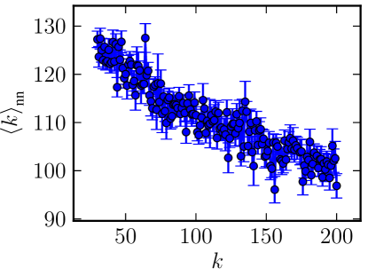
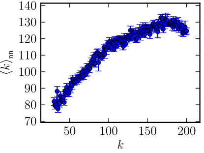
As can be seen in Fig. 2, the degree distribution is broad enough to cause intrinsic dissortative degree correlations in the generated sample. In the following, the same single sample from the ensemble will be used, to mimic the situation of empirically obtained data. However, we have repeated the analysis for different samples from the ensemble, and found always very similar results.

Figure 2: (Color online) Average nearest neighbour degree ${\left<k\right>}_{\text{nn}}(k)$, as a function of the degree of the originating vertex $k$, for the model with intrinsic (left) and extrinsic (right) degree correlations.

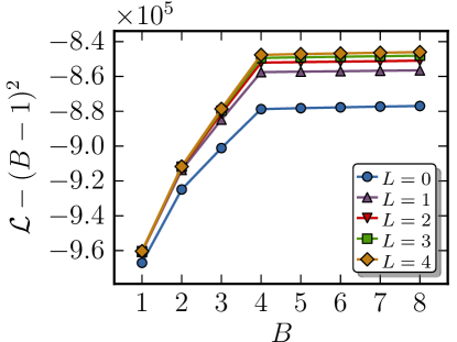
It is usually the case that one does not know a priori which value of $B$ is the most appropriate. Hence, one must obtain the best partitions for several $B$ values, and choose the one with the largest value of $\mathcal{L}$. However, the values of $\mathcal{L}$ will always increase monotonically with $B$, since the number of suitable models will become larger, while the data remains the same, culminating in the extreme situation where each vertex will belong to its own block, and the inferred $e_{rs}$ parameters will be given directly by the adjacency matrix . One can estimate how $\mathcal{L}$ should increase with $B$ by exploiting the fact the first term in Eq. 60 has the same functional form as the mutual information of two random variables $x$, $y$,

$$I(x,y)=\sum_{xy}p_{xy}\ln\left(\frac{p_{xy}}{p_{x}p_{y}}\right),$$ (63)

where $p_{xy}$ is the joint distribution of both variables. It is a known fact that the mutual information calculated from empirical distributions suffers from an upwards systematic bias which disappears only as the number of samples goes to infinity Treves and Panzeri (1995). Assuming the fluctuations of the counts in each bin of the distribution are independent, one can calculate this bias analytically as $\Delta I(x,y)=(X-1)(Y-1)/2N_{s}+O(1/N_{s}^{2})$, where $X$ and $Y$ are the number of possible values of the $x$ and $y$ variables, respectively, and $N_{s}$ is the number of empirical samples Treves and Panzeri (1995). Using this information, one can obtain an estimation for the dependence of $\mathcal{L}$ on $B$,

$$\mathcal{L}^{*}\approx\mathcal{L}-(B-1)^{2},$$ (64)

where $\mathcal{L}^{*}$ is the expected “true” value of the log-likelihood, if the sample size goes to infinity . This can be used to roughly differentiate between situations where the log-likelihood is increasing due to new block structures which are being discovered, and when it is only due to an artifact of the limited data.

In Fig. 3 are shown the values of $\mathcal{L}$ for different $L$, for the same sample of the ensemble above. The likelihood increases monotonically until $B=4$, after which it does not increase significantly. The values of $\mathcal{L}$ are significantly different for different $L$ (which shows that the higher order terms in Eq. 60 should indeed not be neglected), but all curves indicate $B=4$ as being the “true” partition size, which is indeed correct. However, a closer inspection of the resulting partitions reveals important differences. In Fig. 4 are shown some of the obtained partitions for different values of $L$ and $B$. For $B=4$, all values of $L$ result in the same partition, which corresponds exactly to the correct partition. For larger values of $B$, however, the obtained partitions differ a lot more than one would guess by looking at the values of $\mathcal{L}$ alone. For $B=8$ and $L=0$ one sees a clear division into $8$ blocks, which strongly separates vertices of different degrees. This could easily be mistaken for a true partition, despite the fact that it is nothing more than an entropic artifact of the broad degree distribution. Indeed if one increases $L$, the optimal partition becomes eventually a random sub-partition of the correct $B=4$ structure. In this particular example, $L=2$ is enough to obtain the correct result, and the higher values result in the same partition, with only negligible differences.

Figure 3: (Color online) Left: Optimized log-likelihood $\mathcal{L}$ (Eq. 60) as a function of $B$, for different values of $L$, for the same sample from the ensemble with intrinsic degree correlations. Right: Average normalized mutual information (Eq. 65) between the degree sequence and the block partition, as a function of $B$, for different values of $L$.

$B=4,L=\{0,1,2,3,4\}$

$B=8,L=0$

$B=8,L=1$

$B=8,L=2$

$B=8,L=3$

$B=8,L=4$

Figure 4: (Color online) Obtained block partitions for different values of $B$ and $L$, for the same sample of the ensemble with intrinsic degree correlations. The colors indicate the partition, and the size of the vertices is proportional to the degree. Nodes of high degree are pushed towards the center of the layout. Note that for $B=8$ and $L\in[0,1]$, the nodes of high degree are segregated into separate blocks.

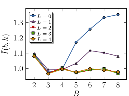
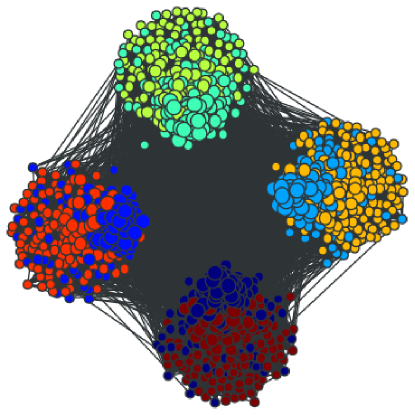
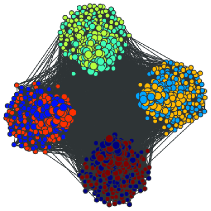
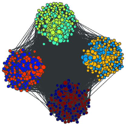
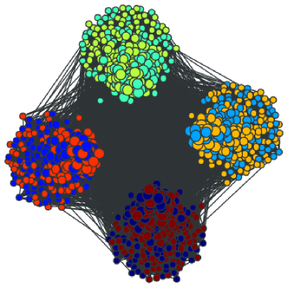
The correlation of the block partition with the degree sequence can be computed more precisely by using the mutual information $I(b,k)$ (Eq. 63), between the block labels and the degrees. Since we want to compare partitions obtained for different values of $B$, and changing $B$ will invariably change $I(b,k)$, we use instead the average normalized mutual information, defined here as,

$$\bar{I}(b,k)=\left<\frac{I(b,k)}{I(r,k)}\right>,$$ (65)

where $I(r,k)$ is the mutual information of the degree sequence and a random block partition $\{r_{i}\}$, obtained by shuffling the block labels $\{b_{i}\}$. The average is taken over several independent realizations of $\{r_{i}\}$. If the block partition is uncorrelated with the degree sequence, one should have that $\bar{I}(b,k)$ is close to one, since there are no intrinsic correlations between the correct partition and the degrees. The values of $\bar{I}(b,k)$ are shown in Fig 3. One sees clearly that the results for lower values of $L$ are significantly correlated with the degree sequence, and that for $L\geq 2$ the correlation essentially vanishes.

The reason why the log-likelihood with $L=0$ delivers spurious block structures is intimately related to the fact that the degree distribution is this case is broad. This causes the remaining terms of Eq. 60 to become relevant, as they represent the entropic cost of an edge leading to a block with a broader degree distribution. On the other hand, the same entropic cost is responsible for the dissortative degree correlations seen in Fig. 2. This is in fact inconsistent with the assumption made when deriving Eq. 16, namely Eq. 15, which says that there are no such degree correlations. This is indeed true, and it means that Eq. 60, even for $L\to\infty$, is still an approximation which neglects certain entropic effects. However, as mentioned previously, it still captures a large portion of the entropic cost of placing an edge incident to a block with a broad degree sequence, and this is the reason why it can be used to infer the correct block structure in the example shown. The same performance should be expected in situations where the intrinsic degree correlations are present, but not “too strong” as to require better approximations. Indeed, as was discussed previously following the derivation of Eq. 16, for networks with very large degrees it may be that Eq. 60 diverges, for sufficiently large $L$. However, this situation can be managed adequately. In Sec. III.2 we computed the entropy for the ensemble with soft degree constraints and arbitrary degree correlations, given in Eq. 10. This expression is exact, and can be used as a log-likelihood in the extreme situations where Eq. 60 is not a good approximation. The downside is that one needs to infer much more parameters, since the model is defined by the full matrix $e_{(r,k),(s,k)}$, which makes the maximization of $\mathcal{L}$ less computationally efficient, and may result in overfitting. A more efficient method will be described in the next section, which consists in separating vertices in groups of similar degree, and using this auxiliary partition to infer the actual block structure. This can be done in way which allows one to control how much information needs to be inferred, such that the degree correlations (intrinsic or otherwise) have been sufficiently accounted for.

VI.2 Extrinsic degree correlations

We consider now the case where there are arbitrary extrinsic degree correlations (although the method described here also works well in situations with strong intrinsic degree correlations which are not well captured by Eq. 60). As an example, we will use a modified version of the blockmodel ensemble used in the previous section, which includes assortative degree correlations, defined as

$$e_{(r,k),(s,k^{\prime})}\propto\frac{e_{rs}}{1+|k-k^{\prime}|},$$ (66)

where $e_{rs}$ is given by Eq. 61. Similarly to the previous case, we consider a typical sample from this ensemble, with $N=10^{3}$ vertices, $B=4$, a block structure with $w=0.99$, and degree distribution with $\gamma=1.1$ and $[k_{\text{min}},k_{\text{max}}]=[30,200]$. The degree correlations obtained in this sample is show in Fig. 2.

$B=4$

$B=8$

Figure 5: (Color online) Inferred block partitions for the model with extrinsic degree correlations, obtained my maximizing the log-likelihood $\mathcal{L}$, given by Eq. 60, for different values of $B$ and $L=2$.

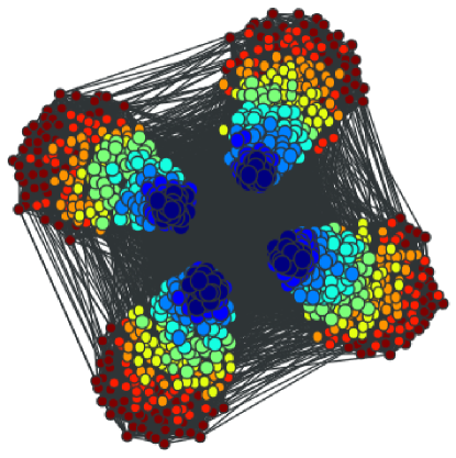
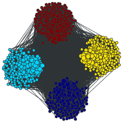
Auxiliary partition $\{d_{i}\}$, with $D=8$.

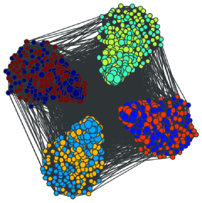
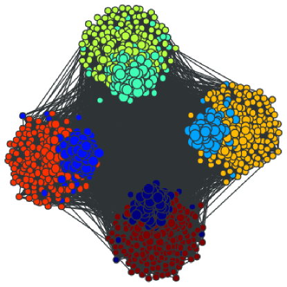
Inferred partition $\{b_{i}\}$, with $B=8$.

Figure 6: (Color online) Auxiliary and inferred block partitions for a sample of the ensemble with intrinsic degree correlations.

Figure 7: (Color online) Left: Optimized log-likelihood $\mathcal{L}$ (Eq. 60) as a function of $B$, for different values of $L$, for the same sample from the ensemble with extrinsic degree correlations. The legend “aux.” indicates results obtained with the auxiliary degree-based partition described in the text. Right: Average normalized mutual information (Eq. 65) between the degree sequence and the block partition, as a function of $B$, for different values of $L$, and size of the auxiliary partition $D$ (or without it if $D$ is omitted).

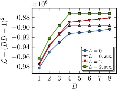
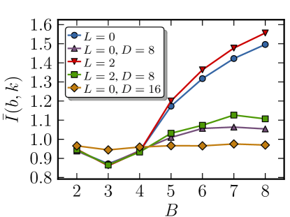
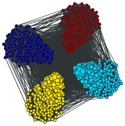
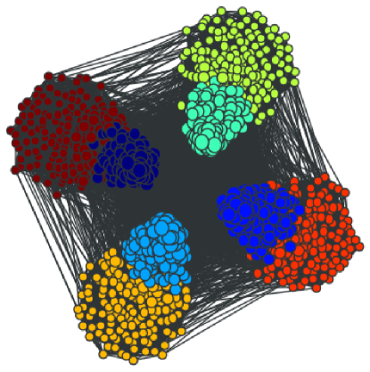
If one does not know, or ignores, that there are degree correlations present, and attempts to detect the most likely block structure using Eq. 60, one obtains block partitions shown in Fig. 5. Due to the high segregation of the modules, one indeed finds the correct block partition for $B=4$, but as the value of $B$ is increased, one finds increasingly many “sub-blocks” corresponding to groups vertices of different degrees. This is simply a manifestation of the degree correlations present in Eq. 66. As Fig. 5 shows, the log-likelihood increases steadily with larger $B$ values, indicating that the “true” block structure has not yet been found. Indeed one would need to make $B\sim 4K$, where $K$ is the number of different degrees in the network, to finally capture the complete structure. The correct inferred partition in this case would put vertices of the same degree in their own block, which we can label as $(r,k)$. In this situation, Eq. 16 becomes no longer an approximation, since Eq. 17 will also hold exactly, and it becomes identical to Eq. 10, which we could use instead as a log-likelihood (which effectively removes the parameter $L$). Strictly speaking, Eq. 10 is entirely sufficient to detect any block structure with arbitrary degree correlations, either intrinsic or extrinsic. In practice, however, it is cumbersome to use since it requires the inference a large amount of parameters, namely the full $e_{(r,k),(r,k)}$ matrix of size $(BK)^{2}$ (of which half the elements are independent parameters), as well as the $n_{(r,k)}$ vector of size $BK$. The number of different degrees $K$ is often significantly large. For the specific example shown in Fig. 5 we have $K=168$, which results in a parameter matrix which is much larger than the number of edges in the network. This is an undesired situation, since with such a large number of parameters, not only it becomes easier to get trapped in local maxima when optimizing $\mathcal{L}$, but also it becomes impossible to discern between actual features of the inferred model and stochastic fluctuations which are frozen in the network structure. However, it is possible to circumvent this problem using the following approach. Before attempting to infer the block partition $\{b_{i}\}$, one constructs an auxiliary partition $\{d_{i}\}$ which remains fixed throughout the entire process. The auxiliary partition separates vertices in $D$ blocks representing degree bins, so that vertices in the same block have similar degrees. Exactly how large should be each degree block, and how the bin boundaries should be chosen will depend in general of specific network properties; however a good starting point is to separate them into bins such that the total number of bins $D$ is as small as possible, while at the same time keeping the degree variance within each bin also small. Furthermore, one should also avoid having degree bins with very few vertices, since this is more likely to lead to artifacts due to lack of statistics. With this auxiliary partition in hand, one can proceed to infer a block partition $\{b_{i}\}$ into $B$ blocks, such that the combined block label of a given vertex $i$ is $(b_{i},d_{i})$. The log-likelihood is computed using Eq. 60, using the full $(b,d)$ block labels to differentiate between blocks. If the $\{d_{i}\}$ partition is reasonably chosen, the degree correlations will be inferred automatically, and from the $\{b_{i}\}$ partition it is possible to extract the block structure which is independent from degree correlations. Note however that after this procedure the $b_{i}$ labels by themselves do not represent a meaningful partition, since any relabeling of the form $(r,d)\leftrightarrow(s,d)$, for the same value of $d$, results in an entirely equivalent block structure. In order to obtain a meaningful $\{b_{i}\}$ partition, it is necessary to proceed as follows,

1. Maximize $\mathcal{L}$ using auxiliary the partition, $\{d_{i}\}$, obtaining the best partition $\{(b_{i},d_{i})\}$.

2. Swap labels $(r,d)\leftrightarrow(s,d)$, within the same auxiliary block $d$, such that the log-likelihood $\mathcal{L}$, ignoring the auxiliary partition $\{d_{i}\}$, is maximized.

In step 2, the labels are swapped until no further improvement is possible. After step 2 is completed, the blockmodel obtained in step 1 remains unchanged, but the block labels $\{b_{i}\}$ now have a clear meaning, since they represent the best overall block structure, ignoring the auxiliary partition, among the possibilities which are equivalent to the inferred block partition.

In the left of Fig. 6 is shown an example auxiliary partition, with $D=8$, and bin widths chosen so that all groups have approximately the same size. On the right is shown the inferred $\{b_{i}\}$ partition with $B=8$, using the auxiliary partition, after the label swap step described above. Notice how the correlations with degree can no longer be distinguished visually. Observing how the log-likelihood increases with $B$ (see Fig. 7), the results with the auxiliary partition point more convincingly to the $B=4$ structure, since it does not increase significantly for increasing block numbers. Fig 7 also shows the average normalized mutual information between the block partitions and the degrees, and indeed the difference between the inference with and without the block partition is significant. For $D=8$ one can still measure a residual correlation, but by increasing the auxiliary partition to $D=16$ virtually removes it, which is still significantly smaller than the total number of degrees $K=168$.

VII Conclusion

We have calculated analytical expressions for the entropy of stochastic blockmodel ensembles, both in its traditional and degree-corrected forms. We have considered all the fundamental variants of the ensembles, including directed and undirected graphs, as well as degree sequences implemented as soft and hard constraints. The expressions derived represent generalizations of the known entropies of random graphs with arbitrary degree sequence Bender (1974); Bender and Butler (1978); Wormald (1999); Bianconi (2009), which are easily recovered by setting the number of blocks to one.

As a straightforward application of the derived entropy functions, we applied them to the task of blockmodel inference, given observed data. We showed that this method can be used even in situations where there are intrinsic (i.e. with an entropic origin) degree correlations, and can be easily adapted to the case with arbitrary extrinsic degree correlations. This approach represents a generalization of the one presented in Karrer and Newman (2011), which is only expected to work well with sparse graphs without very broad degree sequences.

Furthermore, the blockmodel entropy could also be used as a more refined method to infer the relevance of topological features in empirical networks Bianconi et al. (2009), and to determine the statistical significance of modular network partitions Lancichinetti et al. (2010); Radicchi et al. (2010); Lancichinetti et al. (2011).

Beyond the task of block detection, the knowledge of the entropy of these ensembles can be used to directly obtain the equilibrium properties of network systems which possess an energy function which depends directly on the block structure. Indeed this has been used in Peixoto (2012a) to construct a simplified model of gene regulatory system, in which the robustness can be expressed in terms of the block structure, functioning as an energy function. The evolutionary process acting on the system was mapped to a Gibbs ensemble, where the selective pressure plays the role of temperature. The equilibrium properties were obtained by minimizing the free energy, which was written using the blockmodel entropy. This model in particular exhibited a topological phase transition at higher values of selective pressure, where the network becomes assembled in a core-periphery structure, which is very similar to what is observed in real gene networks. We speculate that the blockmodel entropy can be used in the same manner to obtain properties of wide variety of adaptive networks Gross and Blasius (2008), for which stochastic blockmodels are adequate models.

References

- Holland et al. (1983) P. W. Holland, K. B. Laskey, and S. Leinhardt, Social Networks 5, 109 (1983).
- Fienberg et al. (1985) S. E. Fienberg, M. M. Meyer, and S. S. Wasserman, Journal of the American Statistical Association 80, 51 (1985).
- Faust and Wasserman (1992) K. Faust and S. Wasserman, Social Networks 14, 5 (1992).
- Anderson et al. (1992) C. J. Anderson, S. Wasserman, and K. Faust, Social Networks 14, 137 (1992).
- Doreian et al. (2004) P. Doreian, V. Batagelj, and A. Ferligoj, Generalized Blockmodeling (Cambridge University Press, 2004).
- Brandes et al. (2010) U. Brandes, J. Lerner, and U. Nagel, Advances in Data Analysis and Classification 5, 81 (2010).
- Fortunato (2010) S. Fortunato, Physics Reports 486, 75 (2010).
- Newman and Leicht (2007) M. E. J. Newman and E. A. Leicht, Proceedings of the National Academy of Sciences 104, 9564 (2007).
- Reichardt and White (2007) J. Reichardt and D. R. White, The European Physical Journal B 60, 217 (2007).
- Bickel and Chen (2009) P. J. Bickel and A. Chen, Proceedings of the National Academy of Sciences 106, 21068 (2009).
- Guimerà and Sales-Pardo (2009) R. Guimerà and M. Sales-Pardo, Proceedings of the National Academy of Sciences 106, 22073 (2009).
- Karrer and Newman (2011) B. Karrer and M. E. J. Newman, Physical Review E 83, 016107 (2011).
- Ball et al. (2011) B. Ball, B. Karrer, and M. E. J. Newman, Physical Review E 84, 036103 (2011).
- Reichardt et al. (2011) J. Reichardt, R. Alamino, and D. Saad, PLoS ONE 6, e21282 (2011).
- Decelle et al. (2011) A. Decelle, F. Krzakala, C. Moore, and L. Zdeborová, Physical Review E 84, 066106 (2011).
- Peixoto (2012a) T. P. Peixoto, Physical Review E 85, 041908 (2012a).
- Peixoto (2012b) T. P. Peixoto, Journal of Statistical Mechanics: Theory and Experiment 2012, P01006 (2012b).
- Gross and Blasius (2008) T. Gross and B. Blasius, Journal of The Royal Society Interface 5, 259 (2008).
- Newman (2010) M. Newman, Networks: An Introduction (Oxford University Press, 2010).
- Newman (2003a) M. E. J. Newman, Phys. Rev. E 67, 026126 (2003a).
- Girvan and Newman (2002) M. Girvan and M. E. J. Newman, Proceedings of the National Academy of Sciences 99, 7821 (2002).
- Bianconi (2008) G. Bianconi, EPL (Europhysics Letters) 81, 28005 (2008).
- Anand and Bianconi (2009) K. Anand and G. Bianconi, Physical Review E 80, 045102 (2009).
- Bianconi (2009) G. Bianconi, Physical Review E 79, 036114 (2009).
- Anand and Bianconi (2010) K. Anand and G. Bianconi, Physical Review E 82, 011116 (2010).
- Castellano et al. (2009) C. Castellano, S. Fortunato, and V. Loreto, Reviews of Modern Physics 81, 591 (2009).
- Strauss (1986) D. Strauss, SIAM Review 28, 513 (1986).
- Burda et al. (2001) Z. Burda, J. D. Correia, and A. Krzywicki, Physical Review E 64, 046118 (2001).
- Park and Newman (2004a) J. Park and M. E. J. Newman, Physical Review E 70, 066117 (2004a).
- Park and Newman (2004b) J. Park and M. E. J. Newman, Physical Review E 70, 066146 (2004b).
- Palla et al. (2004) G. Palla, I. Derényi, I. Farkas, and T. Vicsek, Physical Review E 69, 046117 (2004).
- Burda et al. (2004) Z. Burda, J. Jurkiewicz, and A. Krzywicki, Physical Review E 69, 026106 (2004).
- Biely and Thurner (2006) C. Biely and S. Thurner, Physical Review E 74, 066116 (2006).
- Fronczak et al. (2006) A. Fronczak, P. Fronczak, and J. A. Hołyst, Physical Review E 73, 016108 (2006).
- Fronczak et al. (2007) P. Fronczak, A. Fronczak, and J. A. Hołyst, The European Physical Journal B 59, 133 (2007).
- Jeong et al. (2007) D. Jeong, M. Y. Choi, and H. Park, Journal of Physics A: Mathematical and Theoretical 40, 9723 (2007).
- Foster et al. (2010) D. Foster, J. Foster, M. Paczuski, and P. Grassberger, Physical Review E 81, 046115 (2010).
- Nowicki and Snijders (2001) K. Nowicki and T. A. B. Snijders, Journal of the American Statistical Association 96, 1077 (2001).
- Bender (1974) E. A. Bender, Discrete Mathematics 10, 217 (1974).
- Bender and Butler (1978) E. Bender and J. Butler, Computers, IEEE Transactions on C-27, 1180 (1978).
- Wormald (1999) N. Wormald, London Mathematical Society Lecture Note Series , 239–298 (1999).
- Chung and Lu (2002a) F. Chung and L. Lu, Proceedings of the National Academy of Sciences 99, 15879 (2002a).
- Chung and Lu (2002b) F. Chung and L. Lu, Annals of Combinatorics 6, 125 (2002b).
- Cover and Thomas (1991) T. M. Cover and J. A. Thomas, Elements of Information Theory, 99th ed. (Wiley-Interscience, 1991).
- Note (1) Because of the similarity of Eq. 12 with the Fermi-Dirac distribution in quantum mechanics, as well as the analogy of the simple graph restriction with the Pauli exclusion principle, this type of ensemble is sometimes called “fermionic”, and conversely the multigraph ensemble of Sec. IV is called “bosonic” Park and Newman (2004a). Note however that the “classical” limit represented by Eq. 15 is still insufficient to make these ensembles equivalent. This is only achieved by the stronger sparsity condition given by Eq. 17.
- Boguñá et al. (2004) M. Boguñá, R. Pastor-Satorras, and A. Vespignani, The European Physical Journal B - Condensed Matter 38, 205 (2004).
- Park and Newman (2003) J. Park and M. E. J. Newman, Physical Review E 68, 026112 (2003).
- Johnson et al. (2010) S. Johnson, J. J. Torres, J. Marro, and M. A. Muñoz, Physical Review Letters 104, 108702 (2010).
- McKay and Wormald (1990) B. McKay and N. Wormald, European J. Combin 11, 565–580 (1990).
- Note (2) Note that not all degree sequences are allowed in the first place, since they must be graphical Erdős and Gallai (1960); Del Genio et al. (2011). Imposing a block structure further complicates things, since the graphical condition needs to be generalized to blockmodels. We will not pursue this here, as we consider only the sufficiently sparse situation, where this issue can be neglected.
- Bollobás (1980) B. Bollobás, Eur. J. Comb. 1, 311 (1980).
- Newman et al. (2001) M. E. J. Newman, S. H. Strogatz, and D. J. Watts, Physical Review E 64, 026118 (2001).
- Newman (2003b) M. E. J. Newman, SIAM Review 45, 167 (2003b).
- King (2004) O. D. King, Physical Review E 70, 058101 (2004).
- Note (3) The difference between ensembles with “hard” and “soft” degree constraints is analyzed in detail in Anand and Bianconi (2010) for the case without block structures.
- Janson (2009) S. Janson, Combinatorics, Probability and Computing 18, 205 (2009).
- Wormald (1981) N. Wormald, Journal of Combinatorial Theory, Series B 31, 168 (1981).
- Holland and Leinhardt (1981) P. W. Holland and S. Leinhardt, Journal of the American Statistical Association 76, 33 (1981).
- Wasserman and Pattison (1996) S. Wasserman and P. Pattison, Psychometrika 61, 401 (1996).
- Zhao et al. (2011) Y. Zhao, E. Levina, and J. Zhu, arXiv:1110.3854 (2011).
- Note (4) We could easily use any of the other entropy expressions derived previously, to accommodate the diverse variants of the ensemble, which could be directed, mutltigraphs, etc. However, the use of the expressions derived for the “hard” degree constraints have a more limited validity, since it assumes stronger sparsity conditions. We focus therefore on ensembles with soft degree constraints, since they are more generally applicable.
- Note (5) This simple method can be very inefficient in certain cases, specially if the network is very large, since one may always finish in local maxima which are far away from the global optimum. We have also used the better variant know as the Kernighan-Lin algorithm Kernighan and Lin (1970), adapted to the blockmodel problem in Karrer and Newman (2011), which can escape such local solutions. However, for the simple examples considered here, we found almost no difference in the results.
- Metropolis et al. (1953) N. Metropolis, A. W. Rosenbluth, M. N. Rosenbluth, A. H. Teller, and E. Teller, The Journal of Chemical Physics 21, 1087 (1953).
- Hastings (1970) W. K. Hastings, Biometrika 57, 97 (1970).
- Taylor (1981) R. Taylor, in Combinatorial Mathematics VIII, Vol. 884, edited by K. L. McAvaney (Springer Berlin Heidelberg, 1981) pp. 314–336.
- Eggleton and Holton (1981) R. B. Eggleton and D. A. Holton, in Combinatorial Mathematics VIII, Vol. 884, edited by K. L. McAvaney (Springer Berlin Heidelberg, 1981) pp. 155–172.
- Coolen et al. (2009) A. C. C. Coolen, A. Martino, and A. Annibale, Journal of Statistical Physics 136, 1035 (2009).
- Note (6) This algorithm actually generates samples from the canonical ensemble, since it allows for fluctuations in the numbers . However, as mentioned in Sec. II, this ensemble is equivalent to the microcanonical version for sufficiently large samples.
- Note (7) An alternative which circumvents this problem is the so-called Maximum A Posteriori (MAP) approach, which uses parameter distributions, instead of a single set of parameters when maximizing the log-likelihood. Instead of the log-likelihood increasing monotonically with , the parameter distributions become broader instead. This approach has been applied to the degree-corrected stochastic blockmodel in Reichardt et al. (2011), using belief propagation. This method, however, has the disadvantage of being numerically less efficient for large networks.
- Treves and Panzeri (1995) A. Treves and S. Panzeri, Neural Computation 7, 399 (1995).
- Note (8) We note that Eq. 64 should be understood only as a rule of thumb which gives a lower bound on the bias of , since it is obtained only from the first term of Eq. 60, and assumes that the number of blocks in each partition fluctuates independently, which is not likely to hold in general since the block partition is a result of an optimization algorithm.
- Bianconi et al. (2009) G. Bianconi, P. Pin, and M. Marsili, Proceedings of the National Academy of Sciences 106, 11433 (2009).
- Lancichinetti et al. (2010) A. Lancichinetti, F. Radicchi, and J. J. Ramasco, Physical Review E 81, 046110 (2010).
- Radicchi et al. (2010) F. Radicchi, A. Lancichinetti, and J. J. Ramasco, Physical Review E 82, 026102 (2010).
- Lancichinetti et al. (2011) A. Lancichinetti, F. Radicchi, J. J. Ramasco, and S. Fortunato, PLoS ONE 6, e18961 (2011).
- Erdős and Gallai (1960) P. Erdős and T. Gallai, Mat. Lapok. 11, 264 (1960).
- Del Genio et al. (2011) C. I. Del Genio, T. Gross, and K. E. Bassler, Physical Review Letters 107, 178701 (2011).
- Kernighan and Lin (1970) B. Kernighan and S. Lin, Bell System Technical Journal 49, 291–307 (1970).