Calculation of the mean duration and age of onset of a chronic disease and application to dementia in Germany

Abstract

This paper descibes a new method of calculating the mean duration and mean age of onset of a chronic disease from incidence and mortality rates. It is based on an ordinary differential equation resulting from a simple compartment model. Applicability of the method is demonstrated in data about dementia in Germany.

Keywords: Chronic diseases; Mean duration; Mean age of onset; Dementia; Incidence; Prevalence; Mortality; Compartment model; Ordinary differential equation.

1 Introduction

This paper deals with analytical methods for calculating the mean age of onset and the mean disease duration in chronic diseases. For this calculation so-called IPM models are used. IPM stands for incidence, prevalence and mortality. First, the general IPM model is introduced. Then, formulas for the mean duration and the mean age of onset of the disease will be developed and applied to epidemiological data about dementia in Germany.

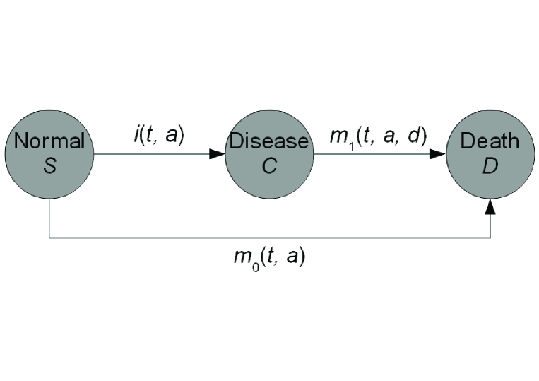
Since we are interested in basic epidemiological parameters such as incidence, prevalence and mortality with respect to a disease, it has proven to be helpful to look at so-called state models (compartmental models). The model that will be used here consists of the three states Normal, Disease, Death and the transitions between the states. Normal means non-diseased with respect to the disease under consideration. The numbers of persons in the Normal and Disease state are denoted as $S$ (susceptible) and $C$ (cases), respectively. The transition intensities (synonymously: rates) are called as shown in Figure 1: $i$ is the incidence rate, $m_{0}$ and $m_{1}$ are the mortality rates of the non-diseased and diseased persons, respectively. In general, the intensities depend on calendar time $t$, age $a$ and sometimes also on the duration $d$ of the disease.

Figure 1: Simple model of a chronic disease with three states. Persons in the state Normal are healthy with respect to the considered disease. In the state Disease they suffer from the disease. The transition rates depend on the calendar time $t,$ on the age $a,$ and in case of the disease-specific mortality $m_{1}$ also on the disease’s duration $d$.

Henceforth, we assume that the rates do not depend on calendar time and not on the duration of the disease. In this situation Murray and Lopez considered a two-dimensional system of ordinary differential equations (ODEs), which expresses the change in the numbers of healthy and sick patients aged $a$ with the corresponding rates, (1994):

$$\begin{split}\frac{\mathrm{d}S}{\mathrm{d}a}&=-\left(i(a)+m_{0}(a)\right)\cdot S\\ \frac{\mathrm{d}C}{\mathrm{d}a}&=i(a)\cdot S-m_{1}(a)\cdot C.\\ \end{split}$$ (1)

Age plays here the role of temporal progression. In the paper (Brinks, 2011) this two-dimensional system is used to derive a scalar ODE of Riccati type, which relates the change in the prevalence at age $a$ to the rates $i$, $m_{0}$ and $m_{1}$:

$$\frac{\mathrm{d}p}{\mathrm{d}a}=(1-p)\cdot\left(i-p\cdot\left(m_{1}-m_{0}\right)\right).$$ (2)

In general, this Ricatti ODE has no closed analytical solution, we have to be contented with numerical solutions. However, there are special cases (e.g. $m_{0}\equiv m_{1}$) in which the ODE is linear, and then there are explicit expressions for the solution.

The benefits of such ODEs are obvious. For given age-specific incidence and mortality rates the age profile of the prevalence can be obtained by solving the Ricatti ODE. Typically this is called the forward or direct problem: we infer from the causes (the rates) to the effect (the prevalence). With smoothness constraints, the incidence and mortality rates determine the prevalence in an unambiguous way.

In addition, for given prevalence and mortality rates the incidence can be dissolved. This is the inverse problem – we conclude from the effect to the cause. This allows, for example, cross-sectional studies being used for incidence estimates, for what otherwise lengthy follow-up studies would be necessary. An example of such an application is shown in (Brinks, 2011).

2 Mean disease duration and median age of onset

In this terminology, formulas for the mean age $\overline{A}$ of onset and the average duration $\overline{D}$ of a chronic disease can be derived. After the preparatory work in the introduction this is now quite simple: For the mean duration $\overline{D}$ the total person time spent in the disease state, i.e. the integral over $C(a)$, has to be divided by the total number of new cases. The total number of new cases is the integral over the product of incidence and number of susceptibles. Hence, it holds

$$\overline{D}=\frac{\int\limits_{0}^{\omega}C(a)\mathrm{d}a}{\int\limits_{0}^{\omega}i(a)\cdot S(a)\mathrm{d}a}=\frac{\int\limits_{0}^{\omega}p(a)\cdot N(a)\mathrm{d}a}{\int\limits_{0}^{\omega}i(a)\cdot(1-p(a))\cdot N(a)\mathrm{d}a},$$ (3)

where $N(a):=S(a)+C(a)$ is the total number of persons in the population with age $a$ and $\omega$ is an age that exceeds the age of the oldest member of the population. In interpreting this expression as the first moment of a random variable $D$, the corresponding variance is

$$\operatorname{Var}(D)=\frac{\int\limits_{0}^{\omega}\left(C(a)-\overline{D}\right)^{2}\mathrm{d}a}{\int\limits_{0}^{\omega}i(a)\cdot S(a)\mathrm{d}a}=\frac{\int\limits_{0}^{\omega}\left(p(a)\cdot N(a)-\overline{D}\right)^{2}\mathrm{d}a}{\int\limits_{0}^{\omega}i(a)\cdot(1-p(a))\cdot N(a)\mathrm{d}a}.$$ (4)

For the mean age $\overline{A}$ of onset, the new cases are weighted by the corresponding age.

$$\overline{A}=\frac{\int\limits_{0}^{\omega}a\cdot i(a)\cdot S(a)\mathrm{d}a}{\int\limits_{0}^{\omega}i(a)\cdot S(a)\mathrm{d}a}=\frac{\int\limits_{0}^{\omega}a\cdot i(a)\cdot\left(1-p(a)\right)\cdot N(a)\mathrm{d}a}{\int\limits_{0}^{\omega}i(a)\cdot(1-p(a))\cdot N(a)\mathrm{d}a},$$ (5)

Correspondingly, the variance of the age of onset is

$$\operatorname{Var}(A)=\frac{\int\limits_{0}^{\omega}\left(a-\overline{A}\right)^{2}\cdot i(a)\cdot S(a)\mathrm{d}a}{\int\limits_{0}^{\omega}i(a)\cdot S(a)\mathrm{d}a}=\frac{\int\limits_{0}^{\omega}\left(a-\overline{A}\right)^{2}\cdot i(a)\cdot\left(1-p(a)\right)\cdot N(a)\mathrm{d}a}{\int\limits_{0}^{\omega}i(a)\cdot(1-p(a))\cdot N(a)\mathrm{d}a}.$$ (6)

Now we have these representations of $\overline{D}$ and $\overline{A}$. Since the age-specific prevalence $p$ is given by the ODE (2), $\overline{D}$ and $\overline{A}$ are completely determined by rates $i,m_{0},m_{1}$ and $N$. It is remarkable, that $\overline{D}$ and $\overline{A}$ depend on the shape $N(a)$ of the age pyramid. One might expect that these numbers are characteristics that just depend on the disease, that they are disease inherent. However, easy considerations show that $\overline{D}$ and $\overline{A}$ have to be dependent on the age-distribution of the population.

The function $N(a)$ is subject of demography. There are in the population models where the numbers of people in the age groups can be represented analytically. The simplest example is the so-called stationary population, (Preston and Coale, 1982), which can for example be obtained from the following conditions:

1. Mortality rates do not depend on calendar time.

2. The birth rate does not depend on calendar time.

3. At each age level, the net migration is 0.

For a stationary population, there are explicit representations for $N(a).$ However, real populations typically are non-stationary, which have to be managed differently. In Germany, there is an official population statistics from the Federal Statistical Office, which captures the age structure of the German population accurately. With $N(a)$ given for every age $a=0,\dots,100+$ from the official statistics, the integrals in Equations (3) – (6) are replaced by sums.

3 Application to dementia in Germany

Our goal now is to apply the tools developed above to epidemiological data about dementia in Germany. The age-specific incidence is taken from (Ziegler and Doblhammer, 2009), which reports data for males and females separately. The mortality $m$ in the German general population is taken from the current life table of the Federal Statistical Office (2011). Reference year is 2010. The relative mortality of the patients is set constant to $R=2.4$, (Rait et al., 2010), as in (Brinks, 2011). In case the general mortality $m$ and the relative mortality $R$ are given, the ODE (2) changes its type and becomes Abelian, (Brinks, 2011, Tab. 1):

$$\frac{\mathrm{d}p}{\mathrm{d}a}=(1-p)\cdot\left\{i-m\cdot\left(1-\left[p\cdot\left(R-1\right)+1\right]^{-1}\right)\right\}.$$ (7)

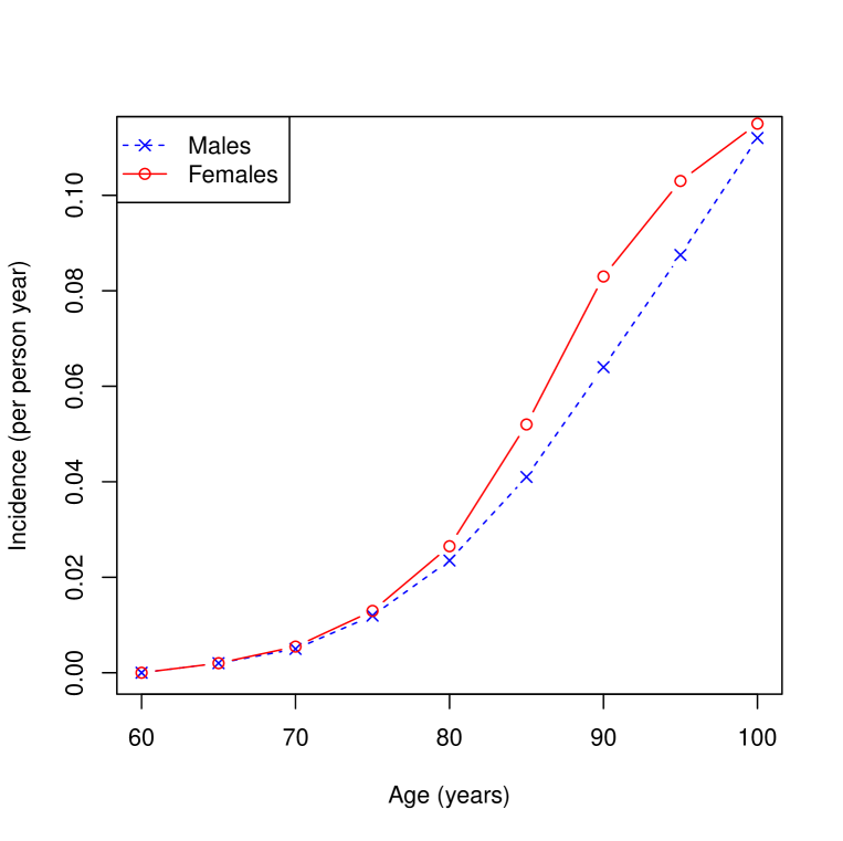
Figure 2 shows the age-specific incidence of dementia for males and females as reported in (Ziegler and Doblhammer, 2009). For this work, the data have interpolated affine-linearly using the middle of the age classes as knots.

Figure 2: Age- and sex-specific incidence of dementia in Germany, (Ziegler and Doblhammer, 2009, Tab. 3).

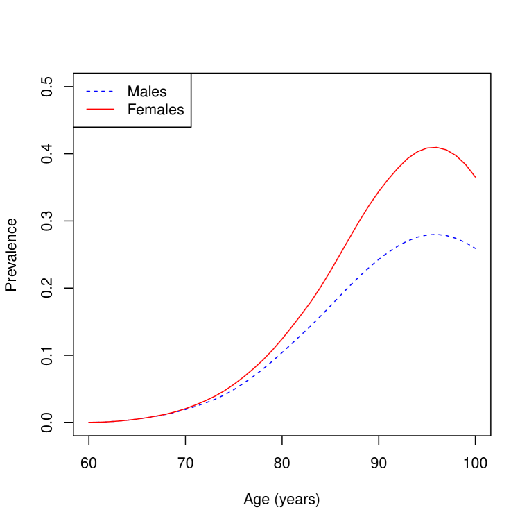
The age-specific prevalence is derived by integrating the Abelian ODE (7) with initial condition $p(60)=0$ via the classical Runge-Kutta method (of fourth order), cf. e.g. (Dahlquist and Björck, 1974). All calculations are performed with the Software R (The R Foundation for Statistical Computing), version 2.12.0. The result is shown in Figure 3.

Figure 3: Age- and sex-specific prevalence of dementia after integration of the ODE (7).

Prevalence at age 60 years starts at 0, which is the initial condition. Until 70 years of age prevalence of men and women are almost the same. In the early 70ies the curves start to diverge, which is likely to be an effect of the different general mortality. Incidence rates in this age class are almost the same for men and women, however general mortality $m$ for men is almost twice as high as for women. A higher general mortality $m_{\text{male}}>m_{\text{female}}$ in Eq. (7) leads to a lower gradient $\tfrac{\mathrm{d}p_{\text{male}}}{\mathrm{d}a}<\tfrac{\mathrm{d}p_{\text{female}}}{\mathrm{d}a}.$ It is striking that both prevalence curves have a maximum at age $a^{\star}=96$ years. At this age it holds $\tfrac{\mathrm{d}p}{\mathrm{d}a}=0$, which implies $i(a^{\star})=p(a^{\star})\cdot m_{0}(a^{\star})\cdot(R-1)$.

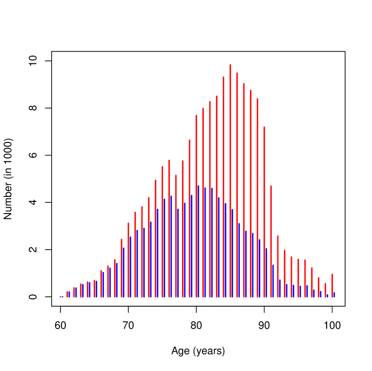
The age distribution of the new cases $i(a)\cdot(1-p(a))\cdot N(a)$ for each age $a=50,\dots,100+$ in 2010 is shown in Figure 4.

Figure 4: Age distribution of the new cases (blue: males, red: females) in 2010 based on the age pyramid $N(a)$ of Germany in the same year.

The modus of the new cases is 80 and 85 years in men and women, respectively. Obviously, women are far more affected than men. The discontinuities stem from the discontinuous structure of the age pyramid.

The corresponding mean age $\overline{A}$ of onset and the mean duration $\overline{D}$ are presented in Table 1.

Table 1: Mean age of onset and duration of dementia in Germany in 2010.

	Mean age $\overline{A}$	Mean duration $\overline{D}$
	(in years)	(in years)
Males	79.3	4.6
Females	82.1	5.4

4 Summary

In this work a simple IPM model has been used to study the mean age of onset and mean duration of a chronic disease. These numbers depend on the incidence of the disease, the mortality of both diseased and non-diseased persons and also on the age pyramid of the population under consideration. The age-specific prevalence inherent in both numbers was obtained as the solution of a new ODE, which has been derived in the predecessor paper (Brinks, 2011). As a practical example, the calculations were applied to data about dementia in Germany. The mean age of onset of dementia is about 79 and 82 years with mean duration 4.6 and 5.4 years in men and women, respectively. Due to the different life expectancies of men and women in Germany, the differences are not surprising. However, it is striking how big the difference in the nubmers of the cases of dementia are. Figure 4 shows the differences in each of the age groups. In the year 2010 a total of about 85000 men and 168000 women aged 65 years and above become diseased. This is in the same order as the 78300 and 166000 males and females reported in (Ziegler and Doblhammer, 2009, Tab. 4) for the year 2007. The reasons for the about doubled number of women compared to men are on the one hand the higher incidence of dementia in females, which leads to a far higher prevalence (see Fig. 3), and on the other hand the higher number of females aged 65+. For comparison, in Germany in 2010 there are 7.2 and 9.6 million men and women aged 65 years and above, respectively.

The methods described here are advantagous to predict characteristics of the persons with dementia. The age of onset might be important for comorbidities (such as diabetes) and associated late complications. The estimated number of diseased persons and disease durations are highly relevant for health services allocation planning. The methods allow predictions on regional levels, too. The age distributions of the states and communities in Germany differ quite substantially, which means that the functions $N(a)$ in the states and communities are different. Hence the associated mean ages of onset and mean durations are different.

This study has some weaknesses. First, the method described needs the incidence and mortality rates being independent from calendar time and disease duration. Both assumptions are hardly fulfilled. Hence, the calculations shown here are just an approximation. Second, the incidences are based on claims data of the statutory health insurance (SHI) from 2002. Beside the fact that the data are old compared to the reference year 2010, SHI data tend to overestimate incidence, (Abbas et al., 2011). Third, the ages equal to and above 100 are summarized in an age class 100+. The reason is the age pyramid of the Federal Statistical Office, which does not stratify ages beyond 100 years.

Another point is worth being mentioned: the examinations in this paper predict a peak in the prevalence of dementia in the second half of the ninth decade of life for men and women. After the peak, prevalence is decreasing again. If sufficient data is available for this age group, this hypothesis can be tested.

References

- Abbas et al. (2011) Abbas, S., Ihle, P., Köster, I., Schubert, I. (2011). Estimation of Disease Incidence in Claims Data Dependent on the Length of Follow-Up: A Methodological Approach. Health Serv Res doi: 10.1111/j.1475-6773.2011.01325.x. [Epub ahead of print]
-
Brinks (2011)
Brinks, R. (2011). A new method for deriving incidence rates from prevalence
data and its application to dementia in Germany.
http://arxiv.org/abs/1112.2720v1 - Dahlquist and Björck (1974) Dahlquist, G., Björck, Å. (1974). Numerical Methods. Upper Saddle River, NJ: Prentice-Hall.
- Federal Statistical Office of Germany (2011) Federal Statistical Office of Germany. (2011). Life table 2008/10.
- Murray and Lopez (1994) Murray, C. J. L. and Lopez, A. D. (1994). Quantifying disability: data, methods and results Bulletin of the WHO 72 (3) 481–494
- Murray and Lopez (1996) Murray, C. J. L. and Lopez, A. D. (1996). Global and regional descriptive epidemiology of disability: incidence, prevalence, health expectancies and years lived with disability. In: Murray, C. J. L., Lopez, A.D. (ed.) The Global Burden of Disease. Boston: Harvard School of Public Health, 201–46.
- Preston and Coale (1982) Preston, S. H. and Coale, A. J. (1982). Age structure, growth, attrition, and accession: a new synthesis, Population Index 48 (2) 217–59
- Preston et al. (2001) Preston, S. H., Heuveline, P. and Guillot, M. (2001). Demography. Malden, MA: Blackwell.
- Rait et al. (2010) Rait, G., Walters, K., Bottomley, C. et al. (2010). Survival of People with Clinical Diagnosis of Dementia in Primary Care, British Medical Journal 341 c3584
- Ziegler and Doblhammer (2009) Ziegler, U., Doblhammer, G. (2009). Prävalenz und Inzidenz von Demenz in Deutschland, Gesundheitswesen 71 281–190