Dynamical System Analysis for Anisotropic Universe in Brans-Dicke Theory

Abstract

In this work, we have studied the Brans-Dicke (BD) cosmology in anisotropic models. We present three dimensional dynamical system describing the evolution of anisotropic models containing perfect fluid and BD scalar field with self-interacting potential. The relevant equations have been transformed into the dynamical system. The critical points and the corresponding eigen values have been found in radiation, dust, dark energy, $\Lambda$CDM and phantom phases of the universe. The natures and the stability around the critical points have also been investigated.

I Introduction

A recent renewal of interest in Brans-Dicke (BD) theory [1] can be traced to the discovery by La and Steinhardt [2] that the use of BD theory in place of general relativity can ameliorate the exit problem of inflationary cosmology. This is possible because the interaction of the BD scalar field with the metric slows the expansion from exponential to power-law. The BD theory contains only one dimensionless parameter, $\omega$ and the effective gravitational constant is inversely proportional to the scalar field $\phi$. BD theory has been proved to be very effective regarding the recent study of cosmic acceleration [3]. This theory yields the correct Newtonian weak-field limit, but solar system measurements of post-Newtonian corrections require $\omega>500$ [4]. In the limit $\omega\rightarrow\infty$, the field $\phi$ becomes a constant [5] and we recover Einstein gravity. This theory has very effectively solved the problems of inflation and the early and the late time behaviour of the Universe. N. Banerjee and D. Pavon [3] have shown that BD scalar tensor theory can potentially solve the quintessence problem. The generalized BD theory [6] is an extension of the original BD theory with a time dependent coupling function $\omega$. In Generalized BD theory, the BD parameter $\omega$ is a function of the scalar field $\phi$. This has led to more general scalar-tensor gravity [7] being considered with a self-interacting potential [8, 9]. Modified BD theory with a self-interacting potential have also been introduced in this regard. Bertolami and Martins [10] have used this theory to present an accelerated Universe for spatially flat model. They have obtained the solution for accelerated expansion with a potential ${\phi}^{2}$ and large $|\omega|$, although they have not considered the positive energy conditions for the matter and scalar field.

Dynamical system theory [11] has been applied with great success in cosmology and astrophysics within the context of general relativity. This theory are used to describe the behaviour of complex dynamical systems usually by constructing differential equations. This theory deals with a long term qualitative behaviour of the formed differential equations. It does not concentrate to find the precise solutions of the system but provide answers like- whether the system is stable for long time and whether the stability depend on the initial conditions. Besides the other scientific fields this theory is now become widely useful in the research of cosmology. Its range of applicability has been enlarged by considering alternate theories of gravity, such as those which do not obey the principle of minimal coupling [12], Kaluza-Klein [13] and scalar-tensor theories [14]. There are several works on qualitative analysis in dynamical system of FRW cosmology in BD gravity [9, 15]. There are some literature where the authors have studied dynamical evolution of some models where the universe is filled with dark energy on an interaction has occurred between dark matter or barotropic matter and some dark energies like Generalized Chaplygin Gas [16], New Generalized Chaplygin Gas[17], ELKO non standard spinor dark energy [18], DBI essence [19], non- minimally coupled scalar field [20], k-essence [21] etc. There are some other approach of dynamical system analysis to diffrent model the universe on the frame work of loop quantum gravity and non linear electro dynamics [22, 23]. Some authors [9, 24] have shown that the field equations for FRW cosmological models could be reduced to a two dimensional dynamical system for any reasonable perfect fluid matter source in BD theory and in the presence of scalar potential, the cosmological dynamical system turns out to be generally three dimensional, apart from radiation dominated universes in which the system once more reduces to two dimensions.

Here we have considered an anisotropic model [25, 26] containing perfect fluid and BD scalar field with self-interacting potential. The starting point of our work is to reduce the field equations to a three dimensional autonomous dynamical system. From the knowledge of mathematical features of the system, we have found the critical points and the exact solutions for the system of equations. Some of the solutions are valid for fluids satisfying the equation of state and for particular values of $\gamma$. The stability around the critical points have been investigated.

II Basic Equations

The self-interacting Brans-Dicke (BD) theory is described by the action: (choosing $8\pi G_{0}=c=1$)

$$S=\int d^{4}x\sqrt{-g}\left[\phi R-\frac{\omega}{\phi}{\phi}^{,\alpha}{\phi,}_{\alpha}-V(\phi)+{\cal L}_{m}\right]$$ (1)

where $V(\phi)$ is the self-interacting potential for the BD scalar field $\phi$ and $\omega$ is the BD parameter. The matter content of the Universe is composed of perfect fluid,

$$T_{\mu\nu}=(\rho+p)u_{\mu}u_{\nu}+p~{}g_{\mu\nu}$$ (2)

where $u_{\mu}~{}u^{\nu}=-1$ and $\rho,~{}p$ are respectively energy density and isotropic pressure.

From the Lagrangian density $(1)$ we obtain the field equations

$$G_{\mu\nu}=\frac{\omega}{{\phi}^{2}}\left[\phi_{,\mu}\phi_{,\nu}-\frac{1}{2}g_{\mu\nu}\phi_{,\alpha}\phi^{,\alpha}\right]+\frac{1}{\phi}\left[\phi_{,\mu;\nu}-g_{\mu\nu}~{}^{\framebox{}}~{}\phi\right]-\frac{V(\phi)}{2\phi}g_{\mu\nu}+\frac{1}{\phi}T_{\mu\nu}$$ (3)

and

$${}^{\framebox{}}~{}\phi=\frac{1}{3+2\omega}T+\frac{1}{3+2\omega}\left[\phi\frac{dV(\phi)}{d\phi}-2V(\phi)\right]$$ (4)

where $T=T_{\mu\nu}g^{\mu\nu}$.

We consider homogeneous and anisotropic space-time model described by the line element

$$ds^{2}=-dt^{2}+a^{2}dx^{2}+b^{2}d\Omega_{k}^{2}$$ (5)

where $a$ and $b$ are functions of time $t$ alone : we note that

$$d\Omega_{k}^{2}=\left\{\begin{array}[]{lll}dy^{2}+dz^{2},~{}~{}~{}~{}~{}~{}~{}~{}~{}~{}~{}~{}\text{when}~{}~{}~{}k=0~{}~{}~{}~{}(\text{Bianchi ~{}I ~{}model})\\ d\theta^{2}+sin^{2}\theta d\phi^{2},~{}~{}~{}~{}~{}\text{when}~{}~{}~{}k=+1~{}~{}(\text{Kantowaski-Sachs~{} model})\\ d\theta^{2}+sinh^{2}\theta d\phi^{2},~{}~{}~{}\text{when}~{}~{}~{}k=-1~{}~{}(\text{Bianchi~{} III~{} model})\end{array}\right.$$

Here $k$ is the curvature index of the corresponding 2-space, so that the above three types are described by Thorne [19] as flat, closed and open respectively.

Now, in BD theory, the Einstein’s field equations for the above space-time symmetry are

$$\frac{\ddot{a}}{a}+2\frac{\ddot{b}}{b}=-\frac{1}{(3+2\omega)\phi}\left[(2+\omega)\rho+3(1+\omega)p\right]-\omega\frac{\dot{\phi}^{2}}{\phi^{2}}-\frac{\ddot{\phi}}{\phi}+\frac{V(\phi)}{2\phi}$$ (9)

$$\frac{\dot{b}^{2}}{b^{2}}+2\frac{\dot{a}}{a}\frac{\dot{b}}{b}=\frac{\rho}{\phi}-\frac{k}{b^{2}}-\left(\frac{\dot{a}}{a}+2\frac{\dot{b}}{b}\right)\frac{\dot{\phi}}{\phi}+\frac{\omega}{2}\frac{\dot{\phi}^{2}}{\phi^{2}}+\frac{V(\phi)}{2\phi}$$ (10)

and the wave equation for the BD scalar field $\phi$ is given by

$$\ddot{\phi}+\left(\frac{\dot{a}}{a}+2\frac{\dot{b}}{b}\right)\dot{\phi}=\frac{1}{3+2\omega}\left[(\rho-3p)-\frac{\phi dV(\phi)}{d\phi}+2V(\phi)\right]$$ (11)

The energy conservation equation is

$$\dot{\rho}+\left(\frac{\dot{a}}{a}+2\frac{\dot{b}}{b}\right)(\rho+p)=0$$ (12)

Here we consider the Universe to be filled with barotropic fluid with EOS

$$p=(\gamma-1)\rho~{},~{}~{}~{}0\leq\gamma\leq 2$$ (13)

The conservation equation $(9)$ yields the solution for $\rho$ as

$$\rho=\rho_{0}\left(ab^{2}\right)^{-\gamma}$$ (14)

where, $\rho_{0}$ is an integration constant.

III Dynamical System Analysis

In this section, we shall define some variables such that the above equations can be transformed to first order differential equations and next we investigate the dynamical system analysis. Let us consider, $V(\phi)=V_{0}\phi^{n+1}$ and define the following variables

$$X=\frac{\phi^{\prime}}{\phi}$$ (15)

$$Y=\frac{1}{3}\left(\frac{a^{\prime}}{a}+2\frac{b^{\prime}}{b}\right)+\frac{\phi^{\prime}}{2\phi}$$ (16)

where,  ${}^{\prime}\equiv\frac{d}{d\eta}\equiv\left(ab^{2}\right)^{1/3}\frac{d}{dt}$ , $\eta$ is the conformal time. If $X>0$ then $Y$ must be positive. If $X<0$ then $Y$ may or may not be positive.

Using the transformations (12) and (13), the equations (6) and (7) become the following two transformed equations (for $k=0$):

$$X^{\prime}+2XY=\left(ab^{2}\right)^{2/3}\left[\frac{(4-3\gamma)}{(3+2\omega)}\frac{\rho}{\phi}-\frac{n-1}{3+2\omega}V_{0}\phi^{n}\right]$$ (17)

$$Y^{\prime}+2Y^{2}=\left(ab^{2}\right)^{2/3}\left[\frac{\{5+3\omega-(2+\omega)\gamma\}}{3+2\omega}\frac{\rho}{\phi}+\frac{(10+6\omega-n)}{6(3+2\omega)}V_{0}\phi^{n}\right]$$ (18)

Also for simplicity, let us choose $n=\frac{2}{3\gamma-2}$ and defining another transformation

$$Z=V_{0}\phi\left(ab^{2}\right)^{\gamma-2/3}~{},$$ (19)

(which is always positive) the above equations reduce to the system of non-linear first order differential equations

$$X^{\prime}+2XY=\frac{4-3\gamma}{3+2\omega}\left[\frac{V_{0}}{Z}-\frac{V_{0}}{3\gamma-2}\left(\frac{Z}{V_{0}}\right)^{\frac{2}{3\gamma-2}}\right]$$ (20)

$$Y^{\prime}+2Y^{2}=\frac{\{5+3\omega-(2+\omega)\gamma\}}{3+2\omega}\frac{V_{0}}{Z}+\frac{\{(3\gamma-2)(5+3\omega)-1\}V_{0}}{3(3+2\omega)(3\gamma-2)}\left(\frac{Z}{V_{0}}\right)^{\frac{2}{3\gamma-2}}$$ (21)

$$Z^{\prime}=(3\gamma-2)ZY-\frac{3\gamma-4}{2}ZX$$ (22)

Now in special cases, we consider radiation, dust, dark energy, $\Lambda$CDM and phantom models and find the critical points, eigen values and its natures separately.

Case (a): Dark Energy: For $\gamma=1/3$, the system of equations (20) becomes

$$X^{\prime}=-2XY+\frac{3V_{0}}{Z(3+2\omega)}+\frac{3V_{0}^{3}}{Z^{2}(3+2\omega)}$$

$$Y^{\prime}=-2Y^{2}+\frac{(13+8\omega)V_{0}}{3Z(3+2\omega)}+\frac{(2+3\omega)V_{0}^{3}}{3Z^{2}(3+2\omega)}$$

$$Z^{\prime}=\frac{3}{2}XZ-YZ$$ (23)

There exists two critical point namely $\left(X_{i}^{DE},Y_{i}^{DE},Z_{i}^{DE}\right)|_{i=1,2}=\left(\mp\frac{\sqrt{2}\beta}{3},\mp\frac{\beta}{\sqrt{2}},\frac{3(5-2\omega)V_{0}^{2}}{16\omega-1}\right)$ where $\beta=\frac{\sqrt{(16\omega-1)(7+5\omega)V_{0}}}{\sqrt{(5-2\omega)\{15-4(\omega-1)\omega\}}}$ and $\frac{1}{16}<\omega<\frac{5}{2}$.

Characteristic Equation around the critical point $\left(X_{i}^{DE},Y_{i}^{DE},Z_{i}^{DE}\right)|_{i=1,2}$ are given by the equation

$$\xi^{3}+A_{1i}\xi^{2}+A_{2i}\xi+A_{3i}=0,~{}~{}~{}~{}~{}~{}~{}i=1,2$$ (24)

where

$$A_{1i}=\pm\frac{\sqrt{2(16\omega-1)(7+5\omega)}}{6(5-2\omega)^{\frac{5}{2}}(3+2\omega)V_{0}^{3}\sqrt{15-4(\omega-1)\omega}}~{}~{}~{}~{}~{}~{}~{}~{}$$

$$A_{2i}=\mp\frac{(16\omega-1)(32\omega^{2}-442\omega-449)}{324(5-2\omega)^{4}(3+2\omega)^{2}V_{0}^{\frac{7}{2}}}~{}~{}~{}~{}~{}~{}~{}~{}~{}i=1,2$$

$$A_{3i}=\mp\frac{(16\omega-1)^{\frac{5}{2}}(7+5\omega)}{81(5-2\omega)^{\frac{7}{2}}(3+2\omega)^{2}V_{0}^{4}\sqrt{2\{15-4(\omega-1)\omega\}}}$$ (25)

The condition for the existence of stable attractor solution for the dynamical system (20) is $A_{1i}>0$, $A_{2i}>0$ and $A_{1i}A_{2i}-A_{3i}>0$ , for $i=1,2$.

In our model, the dynamical system (20) is not stable around $\left(X_{1}^{DE},Y_{1}^{DE},Z_{1}^{DE}\right)$ but stable attractor in the late time universe around the critical point $\left(X_{2}^{DE},Y_{2}^{DE},Z_{2}^{DE}\right)$. Corresponding condition becomes as follows:

$$\frac{(16\omega-1)^{\frac{3}{2}}(7+5\omega)^{\frac{1}{2}}\left\{499+442\omega-32\omega^{2}-12(5-2\omega)^{3}(3+2\omega)(16\omega-1)V_{0}^{\frac{5}{2}}\right\}}{972\sqrt{2}(5-2\omega)^{\frac{13}{2}}(3+2\omega)^{3}V_{0}^{\frac{13}{2}}\{15-4(\omega-1)\omega\}^{\frac{1}{2}}}>0$$ (26)

In particular, for our choice $\gamma=\frac{1}{3},~{}~{}\omega=0.5,~{}~{}V_{0}=0.5$, critical point is $(0.679563,1.01934,0.428571)$ and the corresponding eigenvalues are $(-4.07738,-1.85528,-0.183411)$, which shows a stable attractor. Another critical point is $(-0.679563,-1.01934,0.428571)$, so the system is unstable around that fixed point as the eigenvalues are $(4.07738,1.85528,0.183411)$. The phase space diagram of parameters $X(\eta),Y(\eta),Z(\eta)$ and their progressions have been drawn in figures 1 and 2 respectively.

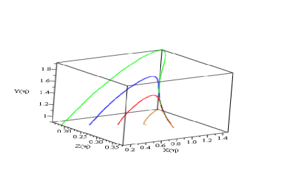
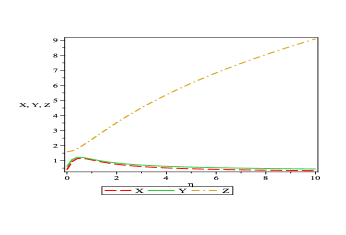
FIG.1                                                                    FIG.2

Figure 1: The phase space diagram of parameters $X(\eta),Y(\eta),Z(\eta)$ for $\gamma=\frac{1}{3},\omega=0.5,~{}~{}V_{0}=0.5$. The initial conditions chosen are $X(0)=0.1$, $Y(0)=0.9$, $Z(0)=0.3V_{0}^{\frac{2}{3}}$ (green); $X(0)=0.2$, $Y(0)=1$, $Z(0)=0.4V_{0}^{\frac{2}{3}}$ (blue); $X(0)=0.3$, $Y(0)=1.1$, $Z(0)=0.5V_{0}^{\frac{2}{3}}$ (red); $X(0)=0.4$, $Y(0)=1.2$, $Z(0)=0.6V_{0}^{\frac{2}{3}}$(brown).

Figure 2: The progression of $X(\eta),Y(\eta),Z(\eta)$ for $\gamma=\frac{1}{3},\omega=0.2,~{}~{}V_{0}=2$ and initial condition is $X(0)=0.4$, $Y(0)=0.6$, $Z(0)=V_{0}^{\frac{2}{3}}$ .

Case (b): Phantom: For $\gamma=-1/2$, the dynamical equation (20) becomes:

$$X^{\prime}=-2XY+\frac{11V_{0}}{2(3+2\omega)Z}+\frac{11V_{0}}{7(3+2\omega)Z}\left(\frac{Z}{V_{0}}\right)^{-\frac{1}{7}}$$

$$Y^{\prime}=-2Y^{2}+\frac{(12+7\omega)V_{0}}{2(3+2\omega)Z}+\frac{(37+21\omega)V_{0}}{21(3+2\omega)Z}\left(\frac{Z}{V_{0}}\right)^{-\frac{1}{7}}$$

$$Z^{\prime}=-\frac{7}{2}YZ+\frac{11}{4}ZX~{}~{}~{}~{}~{}~{}~{}~{}~{}~{}~{}~{}~{}~{}~{}~{}~{}~{}~{}~{}$$ (27)

For $\omega=-\frac{1}{2}$, there exists critical point $(X^{P},Y^{P},Z^{P})$ (superscript $``P"$ stands for phantom) for positive potential function $V_{0}$.

In particular, $\gamma=-\frac{1}{2},~{}~{}\omega=-0.5,~{}~{}V_{0}=4$, critical point is $(2.8606,2.24761,1.497)$ and the corresponding eigenvalues are $(-8.99046,-4.46316,-0.0320722)$, which shows a stable attractor. Another critical point is $(-2.8606,-2.24761,1.497)$ system is unstable around that fixed point as the eigenvalues are $(8.99046,4.46316,0.0320722)$. The phase space diagram of parameters $X(\eta),Y(\eta),Z(\eta)$ and their progressions have been drawn in figures 3 and 4 respectively.

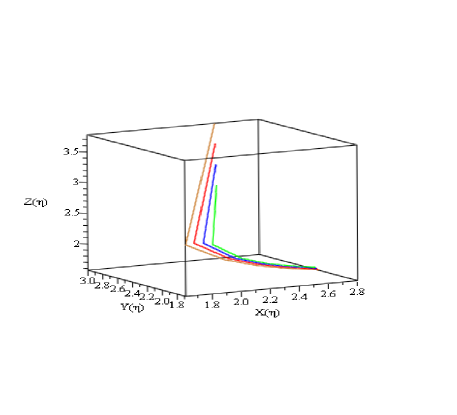
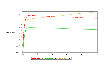
FIG.3                                                                    FIG.4

Figure 3: The phase space diagram of parameters $X(\eta),Y(\eta),Z(\eta)$ for $\gamma=-\frac{1}{2},\omega=-0.5,~{}~{}V_{0}=4$. The initial conditions chosen are $X(0)=2.2$, $Y(0)=2.4$, $Z(0)=1.2V_{0}^{\frac{2}{3}}$ (green); $X(0)=2.3$, $Y(0)=2.6$, $Z(0)=1.3V_{0}^{\frac{2}{3}}$ (blue); $X(0)=2.4$, $Y(0)=2.8$, $Z(0)=1.4V_{0}^{\frac{2}{3}}$ (red); $X(0)=2.5$, $Y(0)=3$, $Z(0)=1.5V_{0}^{\frac{2}{3}}$(brown).

Figure 4: The progression of $X(\eta),Y(\eta),Z(\eta)$ for $\gamma=-\frac{1}{2},\omega=-0.5,~{}~{}V_{0}=2$ and initial condition is $X(0)=0.8$, $Y(0)=0.6$, $Z(0)=V_{0}^{\frac{2}{3}}$ .

Case (c): Radiation: For $\gamma=4/3$, the system of equations (20) becomes

$$X^{\prime}=-2XY~{}~{}~{}~{}~{}~{}~{}~{}~{}~{}~{}~{}~{}$$

$$Y^{\prime}=-2Y^{2}+\frac{Z}{2}+\frac{(7+5\omega)V_{0}}{3Z(3+2\omega)}$$

$$Z^{\prime}=2YZ~{}~{}~{}~{}~{}~{}~{}~{}~{}~{}~{}~{}~{}~{}~{}$$ (28)

From the above dynamical system of equations, we can seen that there is only one feasible critical points namely $(X^{R},0,\sqrt{2\alpha V_{0}})$ ($``R"$ stands for Radiation) where $\alpha=-\frac{7+5\omega}{3(3+2\omega)}$ and the feasible range for $\omega$ becomes $-\frac{3}{2}<\omega<-\frac{7}{5}$, $X^{R}\neq 0$ is arbitrary real constant. In the feasible choice $\gamma=\frac{4}{3},~{}~{}\omega=-1.45,~{}~{}V_{0}=0.5$, only critical point becomes $(0.1,0,0.912871)$, eigen values are $(1.3512,-1.3512,0)$ depicts unstable solution. The phase space diagram of parameters $X(\eta),Y(\eta),Z(\eta)$ and their progressions have been drawn in figures 5 and 6 respectively.

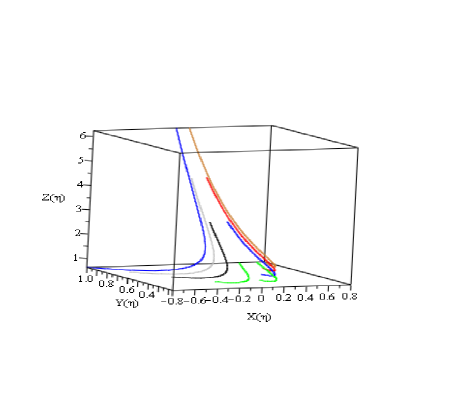
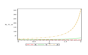
FIG.5                                                                    FIG.6

Figure 5: The phase space diagram of parameters $X(\eta),Y(\eta),Z(\eta)$ for $\gamma=\frac{4}{3},\omega=-1.45,~{}~{}V_{0}=.5$. The initial conditions chosen are $X(0)=0.2$, $Y(0)=0.4$, $Z(0)=V_{0}^{\frac{2}{3}}$ (green); $X(0)=0.4$, $Y(0)=0.6$, $Z(0)=V_{0}^{\frac{2}{3}}$ (blue); $X(0)=0.6$, $Y(0)=0.8$, $Z(0)=V_{0}^{\frac{2}{3}}$ (red); $X(0)=0.8$, $Y(0)=1$, $Z(0)=V_{0}^{\frac{2}{3}}$(brown),$X(0)=-0.2$, $Y(0)=0.4$, $Z(0)=V_{0}^{\frac{2}{3}}$ (green); $X(0)=-0.4$, $Y(0)=0.6$, $Z(0)=V_{0}^{\frac{2}{3}}$ (blue); $X(0)=-0.6$, $Y(0)=0.8$, $Z(0)=V_{0}^{\frac{2}{3}}$ (red); $X(0)=-0.8$, $Y(0)=1$, $Z(0)=V_{0}^{\frac{2}{3}}$(brown).

Figure 6: The progression of $X(\eta),Y(\eta),Z(\eta)$ for $\gamma=\frac{4}{3},\omega=-1.45,~{}~{}V_{0}=1.5$ and initial condition is $X(0)=0.4$, $Y(0)=0.6$, $Z(0)=V_{0}^{\frac{2}{3}}$ .

Case (d): $\Lambda$CDM: For $\gamma=0$, the system of equations (20) becomes

$$X^{\prime}=-2XY+\frac{4V_{0}}{Z(3+2\omega)}+\frac{2V_{0}^{2}}{Z(3+2\omega)}$$

$$Y^{\prime}=-2Y^{2}+\frac{(5+3\omega)V_{0}}{Z(3+2\omega)}+\frac{(11+6\omega)V_{0}^{2}}{6Z(3+2\omega)}$$

$$Z^{\prime}=2XZ-2YZ~{}~{}~{}~{}~{}~{}~{}~{}~{}~{}~{}~{}$$ (29)

From the above dynamical system of equations, we can seen that there is only one feasible critical point namely $(X^{\Lambda},Y^{\Lambda},Z^{\Lambda})$ ($``\Lambda"$ stands for $\Lambda$CDM) where $X^{\Lambda}=Y^{\Lambda}=-\frac{2\sqrt{3(1+3\omega)(4+3\omega)}}{(1-6\omega)\sqrt{Z^{\Lambda}(3+2\omega))}}$, $Z^{\Lambda}>0$ is arbitrary real constant and the feasible range for $\omega$ becomes $-\frac{1}{3}<\omega<\frac{1}{6}$. In the feasible choice $\gamma=0,~{}~{}\omega=-0.1,~{}~{}V_{0}=0.2$, only critical points become $(\pm 0.463304,\pm 0.463304,20.2)$ and the corresponding eigenvalues are $(\mp 1.85322,\mp 0.931517,\pm 0.00490953)$ and so the critical points are unstable. The phase space diagram of parameters $X(\eta),Y(\eta),Z(\eta)$ and their progressions have been drawn in figures 7 and 8 respectively.

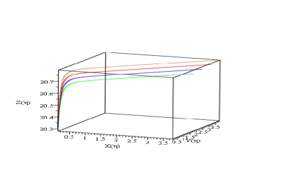
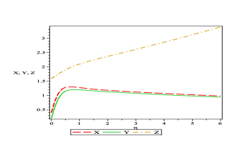
FIG.7                                                                    FIG.8

Figure 7: The phase space diagram of parameters $X(\eta),Y(\eta),Z(\eta)$ for $\gamma=0,\omega=-0.1,~{}~{}V_{0}=.2$. The initial conditions chosen are $X(0)=3.2$, $Y(0)=3.2$, $Z(0)=60.5V_{0}^{\frac{2}{3}}$ (green); $X(0)=3.4$, $Y(0)=3.4$, $Z(0)=60.6V_{0}^{\frac{2}{3}}$ (blue); $X(0)=3.6$, $Y(0)=3.6$, $Z(0)=60.7V_{0}^{\frac{2}{3}}$ (red); $X(0)=3.8$, $Y(0)=3.8$, $Z(0)=60.8V_{0}^{\frac{2}{3}}$(brown).

Figure 8: The progression of $X(\eta),Y(\eta),Z(\eta)$ for $\gamma=0,\omega=-0.2,~{}~{}V_{0}=2$ and initial condition is $X(0)=0.4$, $Y(0)=0.2$, $Z(0)=V_{0}^{\frac{2}{3}}$ .

Case (e): Dust: For $\gamma=1$, the system of equations (20) becomes

$$X^{\prime}=-2XY+\frac{V_{0}}{Z(3+2\omega)}-\frac{Z^{2}}{Z(3+2\omega)V_{0}}$$

$$Y^{\prime}=-2Y^{2}+\frac{V_{0}}{Z}+\frac{Z^{2}(4+3\omega)}{3V_{0}(3+2\omega)}$$

$$Z^{\prime}=\frac{XZ}{2}+YZ~{}~{}~{}~{}~{}~{}~{}~{}~{}~{}~{}~{}$$ (30)

For the dust dominated universe, there are two critical points: $\left(X^{D}_{i},Y^{D}_{i},Z^{D}_{i}\right)|_{i=1,2}$, where $``D"$ stands for dust dominated universe, and given by

$$X^{D}_{1,2}=\mp\frac{\left(\frac{1}{3}\right)^{\frac{1}{6}}\sqrt{2(13+9\omega)V_{0}^{\frac{1}{3}}}}{(7+4\omega)^{\frac{1}{6}}\sqrt{3+2\omega}~{}(5+6\omega)^{\frac{1}{3}}}$$

$$Y^{D}_{1,2}=\mp\frac{\left(\frac{1}{3}\right)^{\frac{1}{6}}\sqrt{(13+9\omega)V_{0}^{\frac{1}{3}}}}{(7+4\omega)^{\frac{1}{6}}\sqrt{2(3+2\omega)}~{}(5+6\omega)^{\frac{1}{3}}}$$

$$Z^{D}_{1,2}=\frac{(21+12\omega)^{\frac{1}{3}}V_{0}^{\frac{2}{3}}}{(5+6\omega)^{\frac{1}{3}}}$$ (31)

Feasible region for existence of these critical point is $\omega>-\frac{5}{6}$. Characteristic roots near the critical point $\left(X^{D}_{1},Y^{D}_{1},Z^{D}_{1}\right)$ are two positive and one negative real roots, and around the critical point $\left(X^{D}_{2},Y^{D}_{2},Z^{D}_{2}\right)$ are two negative and one positive real roots. In the feasible range $\gamma=1,~{}~{}\omega=-0.6,~{}~{}V_{0}=0.2$, critical points are $(\pm 1.28263,\pm 0.641315,0.733281)$, and the corresponding eigen values are $(\mp 3.17407,\pm 0.696701,\mp 0.0878872)$ and so they are unstable. The phase space diagram of parameters $X(\eta),Y(\eta),Z(\eta)$ and their progressions have been drawn in figures 9 and 10 respectively.

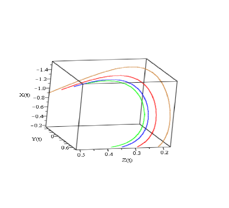
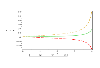
FIG.9                                                                    FIG.10

Figure 9: The phase space diagram of parameters $X(\eta),Y(\eta),Z(\eta)$ for $\gamma=1,\omega=-0.6,~{}~{}V_{0}=.2$. The initial conditions chosen are $X(0)=-1.2$, $Y(0)=-0.2$, $Z(0)=1.2V_{0}^{\frac{2}{3}}$ (green); $X(0)=-1.1$, $Y(0)=-0.3$, $Z(0)=1.3V_{0}^{\frac{2}{3}}$ (blue); $X(0)=-1.0$, $Y(0)=-0.4$, $Z(0)=1.4V_{0}^{\frac{2}{3}}$ (red); $X(0)=-0.9$, $Y(0)=-0.5$, $Z(0)=1.5V_{0}^{\frac{2}{3}}$(brown).

Figure 10: The progression of $X(\eta),Y(\eta),Z(\eta)$ for $\gamma=1,\omega=-0.7,~{}~{}V_{0}=2$ and initial condition is $X(0)=0.4$, $Y(0)=0.6$, $Z(0)=V_{0}^{\frac{2}{3}}$ .

IV Discussions

In this work, we have studied the Brans-Dicke (BD) cosmology in anisotropic models. We present three dimensional dynamical system describing the evolution of anisotropic flat ($k=0$) model containing perfect fluid with barotropic EoS and BD scalar field with self-interacting potential. Choosing the power law form of the potential function $V$ in terms of $\phi$, and defining the three variables $X,~{}Y$ and $Z$, the field equations can be transformed into the dynamical system. The critical points and the corresponding eigen values have been found in radiation, dust, dark energy, $\Lambda$CDM and phantom phases of the universe. The natures and the stability around the critical points have also been investigated. For dark energy case, we have considered $\gamma=\frac{1}{3},~{}~{}\omega=0.5,~{}~{}V_{0}=0.5$, and one critical point is $(0.679563,1.01934,0.428571)$, which is a stable attractor. Another critical point is $(-0.679563,-1.01934,0.428571)$, which is unstable around that fixed point. The 3D phase space diagram of parameters $X,Y,Z$ have been drawn in figure 1 corresponding to the stable critical point. From figure 2, we see that $X$ and $Y$ initially increase and then decrease and $Z$ increases in late stage of the universe. For phantom case, we have taken $\gamma=-\frac{1}{2},~{}\omega=-0.5,~{}V_{0}=4$, and one critical point is $(2.8606,2.24761,1.497)$, which is a stable attractor. Another critical point is $(-2.8606,-2.24761,1.497)$, which is unstable around that fixed point. The 3D phase space diagram of parameters $X,Y,Z$ have been drawn in figure 3 corresponding to the stable critical point. From figure 4, we see that $X$ and $Y$ initially increase and then decrease and $Z$ increases in late stage of the universe. For radiation case, we have considered $\gamma=\frac{4}{3},~{}~{}\omega=-1.45,~{}~{}V_{0}=0.5$, and the only critical point becomes $(0.1,0,0.912871)$ which is unstable. The 3D phase space diagram of parameters $X,Y,Z$ have been drawn in figure 5 corresponding to the critical point. From figure 6, we see that $Y$ and $Z$ increase and $X$ decreases. For $\Lambda$CDM case, we have taken, $\gamma=0,~{}~{}\omega=-0.1,~{}~{}V_{0}=0.2$, and the critical points become $(\pm 0.463304,\pm 0.463304,20.2)$ and these are unstable. The 3D phase space diagram of parameters $X,Y,Z$ have been drawn in figure 7 corresponding to the critical point. From figure 8, we see that $X$ and $Y$ initially increase and then decrease and $Z$ increases in late stage of the universe. For dust case, we have assumed $\gamma=1,~{}~{}\omega=-0.6,~{}~{}V_{0}=0.2$, and the possible critical points are $(\pm 1.28263,\pm 0.641315,0.733281)$ which are unstable. The 3D phase space diagram of parameters $X,Y,Z$ have been drawn in figure 9 corresponding to the critical point. From figure 10, we see that $Y$ and $Z$ increase and $X$ decreases. So the anisotropic model of the universe in Brans-Dicke theory can be stable for some cases of the fluid distribution in late stage of the evolution.

Acknowledgement:

One of the authors (JB) is thankful to CSIR, Govt of India for providing Junior Research Fellowship.

References:

$[1]$ C. Brans and R. H. Dicke, Phys. Rev. 124 925 (1961).
$[2]$ D. A. La and P. J. Steinhardt, Phys. Rev. Lett. 62 376 (1989).
$[3]$ N. Banerjee and D. Pavon, Phys. Rev. D 63 043504 (2001).
$[4]$ C. Will, Theory and Experiments in Gravitational Physics (Cambridge, Cambridge University Press) (1993).
$[5]$ B. K. Sahoo and L. P. Singh, Modern Phys. Lett. A 18 2725- 2734 (2003).
$[6]$ K. Nordtvedt,Jr., Astrophys. J 161 1059 (1970); P. G. Bergmann, Int. J. Phys. 1 25 (1968); R. V. Wagoner, Phys. Rev. D 1 3209 (1970); T. Damour and K. Nordtvedt, Phys. Rev. Lett. 70 2217 (1993); Phys. Rev. D 48 3436 (1993).
$[7]$ P. G. Bergmann, Int. J. Theor. Phys. 1 25 (1968); R. V. Wagoner, Phys. Rev. D 1 3209 (1970).
$[8]$ J. D. Barrow and K. Maeda, Nucl. Phys. B 341 294 (1990).
$[9]$ C. Santos and R. Gregory, Ann. Phys., (NY) 258 111 (1997).
$[10]$ O. Bertolami and P. J. Martins, Phys. Rev. D 61 064007 (2000).
$[11]$ O. I. Bogoyavlensky, Qualitative Theory of Dynamical Systems in Astrophysics and Gas Dynamics (Springer-Verlag, Berlin, 1985).
$[12]$ M. Novello and C. Romero, Gen. Rel. Grav. 19 1003 (1987).
$[13]$ P. Turkowski and K. Maslanka, Gen. Rel. Grav. 19 611 (1987).
$[14]$ V. A. Belinskii et al, Sov. Phys. JETP 62 195 (1986).
$[15]$ C. Romero and H. P. Oliveira, CBPF-NF-045/88, (1988); C. Romero and A. Barros, Gen. Rel. Grav. 25 491 (1993); S. J. Kolitch, Annals Phys. 246 121 (1996); D. J. Holden and D. Wands, Class. Quantum Grav. 15 3271 (1998).
$[16]$ P. Wu and H. Yu, Class. Quantum Grav. 24 4661 (2007); H. Zhang and Z-H Zhu, Phys. Rev. D 73 043518 (2006).
$[17]$ M. Jamil, Int. J. Theor. Phys. 49 62 (2010).
$[18]$ H. M. Sadjadi, arxiv: 1109.1961.
$[19]$ J. Martin and M. Yamaguchi, Phys. Rev. D 77 123508 (2008); B. Gumjudpai, T. Naskar, M. Sami and S. Tsujikawa, JCAP 0506 007 (2005).
$[20]$ O. Hrycyna and M. S. lowski, JCAP 04 026 (2009).
$[21]$ R-J Yang1 and X-T Gao, arxiv: 1006.4968.
$[22]$ K. Xiao and J-Y Zhu, Phys. Rev. D 83 083501 (2011); M. Jamil, D. Momeni and M. A. Rashid, Eur. Phys. J. C 71 1711 (2011); P. Wu and S. N. Zhang, JCAP  bf 0806 007 (2008).
$[23]$R. Garcia-Salcedo, T. Gonzalez, C. Moreno, and I. Quiros, arxiv: 0905.1103.
$[24]$ S. Kolitch and D. Eardley, Ann. Phys. (NY) 241 128 (1995).
$[25]$ S. Chakraborty, N. C. Chakraborty and U. Debnath, Int. J. Mod. Phys. D 11 921 (2002); Int. J. Mod. Phys. A 18 3315 (2003); Mod. Phys. Lett. A 18 1549 (2003).
$[26]$ J. P. Mimoso and D. Wands, Phys. Rev. D 52 5612 (1995); A. Feinstein and J. Ibanez, Class. Quantum Grav. 10 93 (1993).
$[27]$ K. S. Thorne, Astrophys. J. 148 51 (1967).

References:

[1]delimited-[]1[1]