Absorbing states of zero-temperature Glauber dynamics in random networks

Abstract

We study zero-temperature Glauber dynamics for Ising-like spin variable models in quenched random networks with random zero-magnetization initial conditions. In particular, we focus on the absorbing states of finite systems. While it has quite often been observed that Glauber dynamics lets the system be stuck into an absorbing state distinct from its ground state in the thermodynamic limit, very little is known about the likelihood of each absorbing state. In order to explore the variety of absorbing states, we investigate the probability distribution profile of the active link density after saturation as the system size $N$ and $\langle k\rangle$ vary. As a result, we find that the distribution of absorbing states can be split into two self-averaging peaks whose positions are determined by $\langle k\rangle$, one slightly above the ground state and the other farther away. Moreover, we suggest that the latter peak accounts for a non-vanishing portion of samples when $N$ goes to infinity while $\langle k\rangle$ stays fixed. Finally, we discuss the possible implications of our results on opinion dynamics models.

I Introduction

Glauber dynamics Glauber1963 is one of the simplest ways to implement the ordering dynamics of Ising spin systems, which is defined such that detailed balance holds at equilibrium described by the canonical ensemble. When an Ising system evades analytical explanation, we can numerically construct the equilibrium ensemble of the system by running Glauber dynamics until the steady state is reached. However, one may ask whether the ensemble created by Glauber dynamics faithfully represents the equilibrium ensemble of the Ising system, a question that needs to be addressed case by case with caution.

The answer is negative when the dynamics occurs at zero temperature. Lack of noise and the limited range of interaction trap the system in a limited region of phase space, or an absorbing state, from which the ground state with parallel neighboring spins (the only equilibrium configuration at zero temperature) cannot be reached. For regular lattices, such trappings occur whenever the dimension $d$ is greater than 1. For $d=2$, around 30% of systems form stripes of domains and do not evolve any longer Spirin2001+Barros2009 ; Spirin2001a . For $d\geq 3$, an overwhelming fraction of systems fail to reach the ground state. They instead stabilize into states of higher energy and complicated domain shapes Spirin2001a ; Olejarz2011 . The issue of absorbing states has been discussed for other kinds of substrates as well, especially for complex networks in the context of opinion dynamics Svenson2001 ; Haggstrom2002 ; Castellano2005 ; HZhou2005+2007+Castellano2006+Herrero2009 ; Uchida2007 . Here, the relevant question is whether a society can reach a consensus through the local majority rule. The simplest and most studied case is the Erdős–Rényi (ER) Erdos1959+Gilbert1959 random network, which is characterized by the system size $N$ and the average degree $\langle k\rangle$. Earlier numerical studies Svenson2001 ; Castellano2005 ; ERComment have shown that ER networks fail to reach the ground state in some cases. Combinatorial calculations by Häggström Haggstrom2002 proved a stronger statement that the system always fails to reach the ground state in the limit when $N\to\infty$ while $\langle k\rangle$ is finite.

Knowing that the system fails to reach the ground state, we wonder how close the system can get to it. The closeness of the system to the ground state can be represented by the active link density $l_{A}$, which is the fraction of links joining spins of opposite signs as illustrated in Fig. 1. The ground state has $l_{A}=0$, so greater $l_{A}$ indicates that the system is farther away from the ground state. While $l_{A}$ is monotonically decreased by Glauber dynamics at zero temperature, it does not evolve any more once the system gets stuck into an absorbing state. Hence, $l_{A}$ is a natural choice for characterizing an absorbing state.

Häggström Haggstrom2002 showed that $l_{A}$ in an absorbing state has a positive lower bound in the thermodynamic limit, thus proving that full relaxation to $l_{A}=0$ is impossible. There are still more stories to be told about the properties of $l_{A}$. For example, temporal evolution of $l_{A}$ averaged over the systems with $l_{A}\left(t\right)\neq 0$ hints at the existence of at least two groups of samples with very different behaviors of $l_{A}$ (see Fig. 2, where we provide the standard finite-size scaling analysis of the quantity measured by Castellano et al. Castellano2005 ). This leads us to expect that the $l_{A}$ distribution has nontrivial structural features worthy of investigation, which is still lacking.

In this paper, we present a systematic analysis of the absorbing state distribution of $l_{A}$ produced by zero-temperature Glauber dynamics in ER random networks. In particular, we focus on the influence of parameters $N$ and $\langle k\rangle$ on the distribution. The origin of sample-to-sample fluctuations as well as the nature of peaks are also discussed.

The paper is organized as follows. In Sec. II, we briefly describe zero-temperature Glauber dynamics and define quantities of interest. Then, we describe the algorithm proposed by Olejarz et al. Olejarz2011 that ensures the saturation of the system into absorbing states. Our main results, based on extensive numerical simulations, are presented in Sec. III. Finally, we conclude the paper with a summary and discussion in Sec. IV.

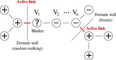
Figure 1: (Color online) An example of a system in which only blinkers are flippable. Active links are highlighted in boldface (red) and the blinker is marked with a question mark “?”. Successive flipping of spins at nodes $V_{1}$, $V_{2}$, …, $V_{n}$ leads to the merger of two domain walls and further relaxation. However, the time required for the process may be long (growing like $n^{2}$), giving a false impression of saturation. This matter is addressed by the acceleration algorithm described in Sec. II.2.

II Model

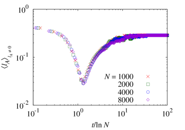
Figure 2: (Color online) Dynamic scaling of $\langle l_{A}\rangle_{l_{A}\neq 0}$ averaged over surviving samples that have never reached the ground state until time $t$. Data collapse very well using the scaling function $\langle l_{A}\rangle_{l_{A}\neq 0}=f(t/\tau)$, where the relaxation time $\tau$ scales as $\tau\sim\ln N$. Numerical data are obtained from $10^{5}$ different network realizations for $\langle k\rangle=10$ as $N$ varies. The dip structure indicates that samples can be divided into two groups: the almost fully-ordered case driving the initial fall and the quickly absorbed case causing the subsequent rise.

II.1 Dynamics and physical quantities

We consider a system consisting of $N$ nodes. Each node is associated with a spin variable $\sigma_{i}$ ($i=1,\ldots,N$) whose value is either $+1$ or $-1$. Pairs of nodes are connected by $L$ randomly distributed links, such that $\langle k\rangle=2L/N$ is the average degree, or the average number of neighbors connected to each node. Let us write $A_{ij}=1$ if nodes $i$ and $j$ are connected, and $A_{ij}=0$ otherwise. An active link is a link joining nodes with oppositely signed spins as shown in Fig. 1. Then, we can define the active link density $l_{A}$ as

$$l_{A}=\frac{1}{L}\sum_{i<j}A_{ij}\frac{1-\sigma_{i}\sigma_{j}}{2}.$$ (1)

We use zero-magnetization initial states with exactly equal numbers of $+1$ and $-1$ spins assigned at random. At each time step, one spin is randomly chosen and updated according to zero-temperature Glauber dynamics, Eq. (2). That is, a spin flips (changes sign) with the following probability, where $\Delta l_{A}$ is the change of $l_{A}$ resulting from the flip.

$$\text{Flipping probability}=\left\{\begin{array}[]{rl}1,&\text{if~{}}\Delta l_{A}<0\\ 1/2,&\text{if~{}}\Delta l_{A}=0\\ 0&\text{if~{}}\Delta l_{A}>0\end{array}\right.$$ (2)

Zero-temperature Glauber dynamics forbids the increase of $l_{A}$. Thus, spins aligned with the majority of its neighbors are “unflippable.” To improve the efficiency of our simulations, we employ the rejection-free technique: instead of updating one spin among all the $N$ spins, we only update one of the flippable spins at each time step. The Monte Carlo simulation (MCS) time should then be increased by $1/\left(\text{number of active spins}\right)$ per update, in order for a fair comparison with the case when the rejection-free technique is not used.

II.2 Saturation test: absorbing states

When zero-temperature Glauber dynamics cannot lower $l_{A}$ any further, we say that the system has reached an absorbing state. If the system has run out of flippable spins, it is certainly in an absorbing state since the dynamics has stopped. There are, however, absorbing states with flippable spins whose neighbors are equally split between $+1$ and $-1$. Such spins are called blinkers as they repeatedly flip back and forth. The existence of blinkers makes the problem of finding an absorbing state trickier.

Blinkers can mislead one to believe that the system has saturated to an absorbing state, while $l_{A}$ can still be lowered as the dynamics continues. Figure 1 illustrates this point. It shows a system in which a single blinker is the only flippable spin at the moment. The blinker can “hop” randomly back and forth between nodes $V_{1}$ and $V_{n}$, which is effectively a random domain wall motion conserving $l_{A}$. If the random-walk domain wall happens to collide with the frozen domain wall on the opposite side of the network, the system can go under further relaxation, $l_{A}$ eventually going to zero. Hence, the network in Fig. 1 has not reached an absorbing state yet. The domain wall collision, however, takes some time (proportional to $n^{2}$) due to the randomness of the domain wall motion. Until the collision occurs, one may get a false impression that $l_{A}$ has saturated and the system has reached an absorbing state. In order to determine whether an apparent saturation of $l_{A}$ truly indicates an absorbing state, we employ the algorithm proposed by Olejarz et al. Olejarz2011 as follows:

1. Until some prescribed MCS time $T$, let the system evolve with zero-temperature Glauber dynamics.

2. Apply a global infinitesimal field, so that blinkers favor one sign over the other and the domain walls composed of blinkers are driven in a biased direction. The field must not be too strong, lest it should make unflippable spins flippable or flippable spins unflippable. The field is maintained until domain walls collide to decrease $l_{A}$, or until the system completely runs out of flippable spins even in the presence of the field. Reverse the global field and do the same.

3. If $l_{A}$ never decreased in the previous step, the system has saturated to an absorbing state and the algorithm terminates. Otherwise, return to the previous step.

To observe the unbiased distribution of absorbing states induced purely by zero-temperature Glauber dynamics, one has to determine $T$ such that no lowering of $l_{A}$ occurs after applying the acceleration algorithm. This is quite a time-consuming task. So we just accept the absorbing state found by the acceleration algorithm even if the algorithm has lowered $l_{A}$. This inevitably biases the absorbing state distribution of $l_{A}$, but we have made sure that the change in the distribution is negligible if $T$ is larger enough than $\tau$. Here, we set $T=100\ln N$.

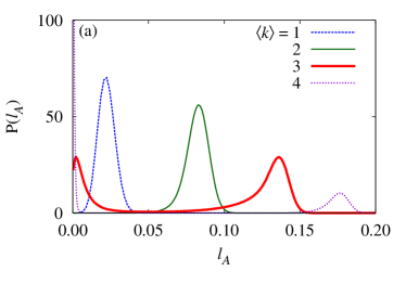
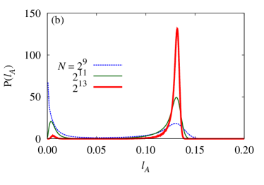
Figure 3: (Color online) Probability distribution functions of $l_{A}$ in absorbing states (a) at $\langle k\rangle=1,\ 2,\ 3,\ 4$ with $N=2^{10}$ and (b) at $N=2^{9},\ 2^{11},\ 2^{13}$ with $\langle k\rangle=3$. Numerical data are obtained from $10^{2}$ zero-magnetization initial configurations and $10^{5}$ network realizations. The $l_{A}$ distribution is essentially bimodal, which implies that it is a mixture of two components that need to be analyzed separately.

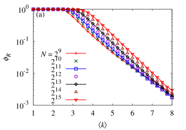
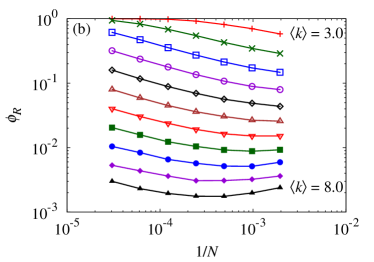
Figure 4: (Color online) The fraction of samples belonging to the right component, $\phi_{R}$, is calculated from the $l_{A}$ distribution. (a) If $N$ is fixed, the value of $\phi_{R}$ decreases with $\langle k\rangle$. (b) If $\langle k\rangle$ is fixed, $\phi_{R}$ eventually increases with $N$. Larger $N$ is required at greater $\langle k\rangle$ to observe the increasing trend. The lines are a guide to the eyes.

III Numerical results

Utilizing the acceleration algorithm to find true absorbing states of zero-temperature Glauber dynamics in ER networks, we obtain the probability distribution function $P\left(l_{A}\right)$ of the active link density $l_{A}$ in absorbing states through extensive numerical simulations covering both different runs on a given ER network and different network realizations. $P\left(l_{A}\right)$ is typically bimodal with the left peak near $l_{A}=0$ and the right peak at a larger value of $l_{A}$ (see Fig. 3). Such a shape of the distribution is consistent with the temporal behavior of $\langle l_{A}\rangle_{l_{A}\neq 0}$ in Fig. 2: both imply that there are two groups of samples with very different properties. From this perspective, we analyze $P\left(l_{A}\right)$ assuming that the distribution always consists of two components, the left and the right. $P\left(l_{A}\right)$ may appear unimodal in some cases, as illustrated by the curves at $\langle k\rangle=1$ and $\langle k\rangle=2$ in Fig. 3(a). Even in such cases, we can assume that there is an unobserved peak of zero (or extremely small) magnitude. An example is shown in Fig. 3(b), where the left peak seems to shrink indefinitely as $N$ grows, leaving only the right peak to be observed.

In the following subsections, we systematically investigate the finite-size effect on $P\left(l_{A}\right)$ with the goal of obtaining the shape of the distribution in the thermodynamic limit. We present numerical evidence that the $l_{A}$ distribution consists of at most two delta peaks in the thermodynamic limit, and that a nonvanishing proportion of samples belongs to the right peak. Clues as to the nature of the peaks and the origin of sample-to-sample fluctuations of $l_{A}$ are also discussed. Finally, we provide evidence that $P\left(l_{A}\right)$ may have only a single delta peak far from $l_{A}=0$ in the thermodynamic limit.

III.1 Proportions of components

We begin our analysis with the finite-size effect on the fraction $\phi_{R}$ of samples belonging to the right component of the $l_{A}$ distribution. The component corresponds to samples stuck far away from the ground state, so higher $\phi_{R}$ indicates greater difficulties in reaching the ground state. We are also interested in whether the $l_{A}$ distribution is still bimodal in the asymptotic limit.

Measurement of $\phi_{R}$ requires the criterion for distinction between the two components of the $l_{A}$ distribution. Without loss of generality, we choose the local minimum point $l_{\text{min}}$ between the maximum point of the left peak $l_{\text{max}}^{L}$ and the maximum point of the right peak $l_{\text{max}}^{R}$ as the border between two peaks. Therefore, $\phi_{R}$ is the fraction of samples ending up on the right side of $l_{\text{min}}$. If there are multiple candidates for $l_{\text{min}}$, the largest (rightmost) one is chosen for a conservative estimation of $\phi_{R}$.

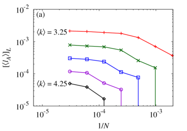
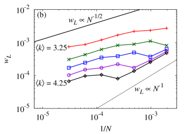
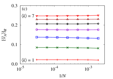
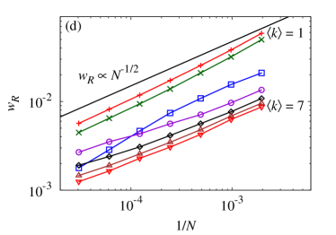
Figure 5: (Color online) The means and widths of two peaks of $P\left(l_{A}\right)$ are measured. (a) The left-peak mean $[\langle l_{A}\rangle]_{{}_{L}}$ is plotted at $\langle k\rangle=3.25,\ldots,4.25$ increased by $0.25$ from top to bottom. (b) The left-peak width $w_{{}_{L}}$ is plotted for the same parameter sets as (a). (c) The right-peak mean $[\langle l_{A}\rangle]_{{}_{R}}$ is plotted for $\langle k\rangle=1,\ldots,7$ increased by $1$ from bottom to top. (d) The right-peak width $w_{{}_{R}}$ is plotted for the same parameter sets as (c). Note that the curves at $\langle k\rangle=1,\ 2$ have been vertically shifted by respective factors of $4$ and $5$ to avoid overlapping with other data. All the data are obtained from $10^{3}$ different initial configurations and $10^{3}$ network realizations. The lines are guide to the eyes.

According to Fig. 4(a), $\phi_{R}$ decreases monotonically with $\langle k\rangle$ when $N$ is fixed. This is a natural consequence of the fact that nodes are better informed of the global situation when the connectivity is greater. On the other hand, $\phi_{R}$ has a nonmonotonic dependence on $N$ when $\langle k\rangle$ is fixed, as in Fig. 4(b). $\phi_{R}$ eventually increases with $N$, which implies that the right-peak component accounts for a nonvanishing portion of samples in the thermodynamic limit. We note that the crossover occurs at greater $N$ as $\langle k\rangle$ gets larger, so observing highly connected networks of small sizes may mislead one to conclude that the right component becomes negligible in the thermodynamic limit. The behavior of $\phi_{R}$ at greater $N$ shows that this is not likely to be the case. On the contrary, one may even claim from our result that the right peak is actually the only observed peak in the thermodynamic limit, as can be numerically confirmed for sufficiently small $\langle k\rangle$. We shall get back to this bold claim later, providing more numerical evidences. For now, we simply interpret the numerical observation for $\phi_{R}$ as evidence that the right component is not an artifact due to the finite-size effect.

III.2 Means and widths of peaks

Now we take a closer look at the shape of $P\left(l_{A}\right)$, and measure the finite-size effect on positions and widths of the two peaks, which are defined as follows. Three extrema ($l_{\text{max}}^{L},\ l_{\text{max}}^{R},\ l_{\text{min}}$) defined in the previous subsection divide the domain of $l_{A}$ into four intervals. The medians of the intervals are denoted by $l_{1}<l_{2}<l_{3}<l_{4}$ in the ascending order. Then, the width of the left (right) peak is defined as $w_{L}=l_{2}-l_{1}$ ($w_{R}=l_{4}-l_{3}$), and the position is represented by the mean value $\left[\langle l_{A}\rangle\right]_{L}$ ($\left[\langle l_{A}\rangle\right]_{R}$) which is the average of $l_{A}$ among samples belonging to the interval between $l_{1}$ and $l_{2}$ ($l_{3}$ and $l_{4}$). The behaviors of those peak properties are plotted in Fig. 5. We note that both peaks are self-averaging: the mean values show signs of saturation, and the widths seem to decay asymptotically like $N^{-1/2}$. Hence, in the thermodynamic limit, we claim that almost all the samples belong to two sharp peaks whose positions are determined solely by $\langle k\rangle$. Here follows detailed descriptions for the analysis of each peak.

III.2.1 Analysis of the left peak

We present the left-peak properties for a rather limited range $3.25<\langle k\rangle<4.25$, due to the following limitations of our study. The left peak may not be observed for small values of $\langle k\rangle$ as shown in Figs. 3(a) and 4, so its properties cannot be measured in such cases. On the other hand, the left peak is too sharp and too close to zero for large values of $\langle k\rangle$, so we hit the resolution limit of peak position and width. In such cases, the left-peak properties show the trivial behavior of a peak of unit width (proportional to $1/N\langle k\rangle$) located at $l_{A}=0$.

Figure 5(a) shows that the value of $[\langle l_{A}\rangle]_{L}$ decreases with $\langle k\rangle$, and approaches positive limits as $N$ grows. This is consistent with the lower bound of $l_{A}$ in the thermodynamic limit derived by Häggström Haggstrom2002 which is positive and decreases with $\langle k\rangle$ in the parameter range observed in our simulations. The vertical drops of $l_{A}$ indicate that the peak becomes too sharp and too close to zero at smaller values of $N$, so $[\langle l_{A}\rangle]_{L}$ becomes indistinguishable from zero in those ranges.

Figure 5(b) shows that the value of $w_{L}$ has a crossover between two scaling regimes: $N^{-1}$ and $N^{-1/2}$. As pointed out in previous paragraphs, the left peak is so narrow for small values of $N$ that its width is just given by the unit of $l_{A}$, which is inversely proportional to $N$. As $N$ gets larger, the unit of $l_{A}$ decays faster than the true peak width, revealing the $N^{-1/2}$ dependence. This crossover to the true scaling regime occurs for the larger values of $\langle k\rangle$ as $N$ gets larger, which is obviously related to the shifting of vertical lines in Fig. 5(a), implying that the two artifacts are of the same origin.

III.2.2 Analysis of the right peak

The right-peak properties are presented for a wider range of parameters, as the limitations present in the case of left-peak properties are not as severe. For the sake of clarity, we have reduced the resolution of $\langle k\rangle$ compared to the case of the left peak.

While Fig. 5(c) clearly shows that $[\langle l_{A}\rangle]_{R}$ saturates as $N$ grows and increases with $\langle k\rangle$, $w_{R}$ exhibits more complicated behaviors as shown in Fig. 5(d). For $\langle k\rangle>3$, the curves seem to follow the $N^{-1/2}$ scaling at small $N$, but deviate from it as $N$ grows. On the other hand, for $\langle k\rangle<3$, the curves are increasingly well-fitted by $N^{-1/2}$ as $N$ increases. We claim that $w_{R}$ decays somewhat like $N^{-1/2}$, but deviates from it around the regime where the left peak is just about to disappear (or, equivalently, just about to appear). The data for $\langle k\rangle=3$ in Fig. 5(d) and the distribution shapes in Fig. 3(b) give a nice illustration of our claim. When $N$ is small, the two peaks are clearly distinguishable, so the $N^{-1/2}$ behavior is easily observed. As $N$ grows, the left peak dwindles and the left component becomes indistinguishable from the right component of the $l_{A}$ distribution. This makes $w_{R}$ appear broader than it really is as we include part of the left component in the right component by mistake, hence $w_{R}$ appears to decay slower than $N^{-1/2}$. As $N$ grows more, the left peak becomes completely unobservable, causing the rapid width decay and the subsequent return to the $N^{-1/2}$ behavior. If we had observed the system at greater $N$, the curve for $\langle k\rangle=7$ would also have shown the rapid width decay and the subsequent return to the $N^{-1/2}$ behavior as was shown by the curve for $\langle k\rangle=3$.

Taking all those considerations into account, we conclude that both components of $P\left(l_{A}\right)$ are self-averaging.

III.3 Nature of the peaks

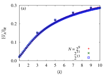
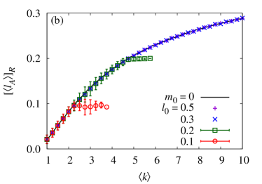
Figure 6: (Color online) (a) The right-peak mean of $l_{A}$ measured for $10^{7}$ ER network samples (lower points) and $10^{6}$ regular random network samples (upper points). Lack of degree fluctuations in odd-degree regular random networks does not make much difference in the right-peak mean, while the right peak completely disappears in even-degree regular random networks. (b) The same quantity measured for different initial magnetization $m_{0}$ or initial active link density $l_{0}$ in $10^{6}$ ER network samples. The result suggests that for each value of $\langle k\rangle$, the right peak corresponds to the only stable spin configurations with approximately zero magnetization.

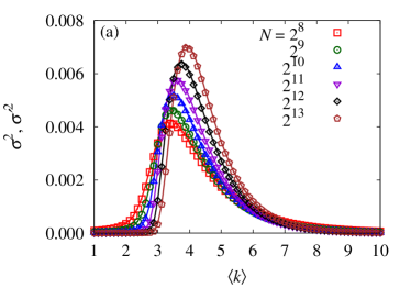
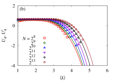
Figure 7: (Color online) Samplet-to-sample fluctuations caused by the contributions of network structure and initial spin configuration are measured for $10^{2}$ initializations of $10^{5}$ network realizations. (a) Variances of $l_{A}$ measured in two different ways (refer to the main text for details) agree well with each other, implying that the mean of $l_{A}$ distribution is unaffected by the exact structure of each particular ER network. (b) A similar result is observed for Binder cumulants of $l_{A}$. Here open symbols represent $\left(\sigma^{2},~{}U_{4}\right)$ and solid lines represent $\left(\sigma^{\prime 2},~{}U_{4}^{\prime}\right)$, respectively.

Based on the results presented so far, we claim that the $l_{A}$ distribution in the thermodynamic limit can be represented as a combination of at most two delta peaks. The nature of the left peak is easily understood: it represents the samples that almost reach the ground state, with a small (but still finite) fraction of active links connecting dangling parts of the system. However, we pose the following question: why should there be another well-defined peak at a much larger value of $l_{A}$?

In order to check whether the ER network is the only substrate with the observed right-peak behavior, we also test zero-temperature Glauber dynamics in the regular random network where all nodes have the same degree $k$. The results are shown in Fig. 6(a). It is remarkable that zero-temperature Glauber dynamics in even-degree regular random networks never produces any “right peak” (only a single peak is formed at or around $l_{A}=0$, which may be called the “left peak”), which is why the data are not plotted at even values of $\langle k\rangle$. This seems to be due to large fluctuations provided by blinkers that can appear only in even-degree nodes. On the other hand, odd-degree regular random networks produce results very similar to ER networks. Lack of degree fluctuations in odd-degree regular random networks yields only small vertical offsets of $[\langle l_{A}\rangle]_{R}$, not significantly altering the right-peak properties observed in ER networks.

To get some hints as to whether the location of $[\langle l_{A}\rangle]_{R}$ has any physical meaning, we compare $[\langle l_{A}\rangle]_{R}$ obtained from the previous simulations in ER networks (whose initial magnetizations are zero, $m_{0}=0$) with the same quantity obtained from initial states characterized by the initial active link density $l_{0}$. For the sake of convenience, let us denote the latter by a new notation $[\langle l_{A}\rangle]_{R}^{l}$. Since $l_{A}$ always decreases with time in Glauber dynamics, samples initialized by $l_{0}$ cannot produce right peaks at values of $l_{A}$ larger than $l_{0}$. Therefore, if $[\langle l_{A}\rangle]_{R}$ observed in the previous results are truly special, we expect a drastic difference in the behavior of $[\langle l_{A}\rangle]_{R}^{l}$ between the samples with $l_{0}>[\langle l_{A}\rangle]_{R}$ and those with $l_{0}<[\langle l_{A}\rangle]_{R}$ since the former can produce a peak around $[\langle l_{A}\rangle]_{R}$ while the latter cannot.

Before moving on to the discussion of results, a remark on the preparation of samples with $l_{0}$ is in order. Those samples are constructed from zero-magnetization spin configurations by random flippings of spins that decrease $\left|l_{A}-l_{0}\right|$. It should be noted that this method does not scan the entire configuration space of the samples characterized by $l_{0}$, since the magnetization of each sample prepared by the method is likely to be very close to zero. However, since the samples belonging to the right component have magnetization close to zero in the absorbing states, our initialization method still serves the purpose of generating samples that are similar to the right-component samples but different only in the value of $l_{A}$.

Figure 6(b) indeed confirms our previously described expectation: the samples with $l_{0}>[\langle l_{A}\rangle]_{R}$ have $[\langle l_{A}\rangle]_{R}^{l}=[\langle l_{A}\rangle]_{R}$, while the right peak disappears in the samples with $l_{0}<[\langle l_{A}\rangle]_{R}$ (the right peak may still remain for a few more steps of $\langle k\rangle$ as the right peak produced by samples with $m_{0}=0$ does have a tail to the left of $\left[\langle l_{A}\rangle\right]_{R}$, which is smaller than $l_{0}$). This indicates that the value of $\left[\langle l_{A}\rangle\right]_{R}$ is indeed physically meaningful since it is the only value of active link density that can be sustained when the magnetization of the system is close to zero.

III.4 Origin of sample-to-sample fluctuations

Now we discuss how the fate of each sample is determined, or what determines whether the system evolves into the left or the right component of the $l_{A}$ distribution. Such sample-to-sample fluctuations come from three factors: different network structures, different initial configurations, and the stochasticity of dynamics.

We separate the effect of network structure from that of the other factors. A natural parameter describing the broadness of the $l_{A}$ would be its variance, which we may define in the following two ways:

$$\sigma^{2} =\left[\langle l_{A}^{2}\rangle\right]-\left[\langle l_{A}\rangle\right]^{2},$$

$$\sigma^{\prime 2} =\left[\langle l_{A}^{2}\rangle-\langle l_{A}\rangle^{2}\right].$$

Here, $\left[\ldots\right]$ represents an average over different network realizations, and $\langle\ldots\rangle$ represents an average over the other factors sharing the common network structure. Therefore, $\sigma^{2}$ is the variance of $l_{A}$ that does not distinguish between contributions from the three factors mentioned above. On the other hand, $\sigma^{\prime 2}$ is the different variance of $l_{A}$ due to different initial configuration and the stochasticity of dynamics, averaged over different network realizations in the final step of calculation. The difference between $\sigma^{2}$ and $\sigma^{\prime 2}$ can be interpreted as the fluctuations of $l_{A}$ solely due to differences in the network structure. Strictly speaking, $\sigma^{2}=\sigma^{\prime 2}$ implies that $\langle l_{A}\rangle$ is the same, irrespective of the exact structure of ER networks as proven below,

$$\sigma^{\prime 2}-\sigma^{2} =\left[\langle l_{A}\rangle^{2}\right]-\left[\langle l_{A}\rangle\right]^{2}$$

$$=\left[\left(\langle l_{A}\rangle-\left[\langle l_{A}\rangle\right]\right)^{2}\right]=0,$$

$$\langle l_{A}\rangle =\left[\langle l_{A}\rangle\right].$$

Figure 7(a) shows that $\sigma^{2}$ and $\sigma^{\prime 2}$ are close to each other for various combinations of $N$ and $\langle k\rangle$. Therefore, the network structure does not contribute much to the mean values of $l_{A}$. The same can be said for the higher moments of $l_{A}$, such as Binder cumulants $U_{4}$ and $U^{\prime}_{4}$,

$$U_{4} =1-\frac{\left[\langle l_{A}^{4}\rangle\right]}{3\left[\langle l_{A}^{2}\rangle\right]^{2}},$$

$$U^{\prime}_{4} =1-\frac{\left[\langle l_{A}^{4}\rangle\right]}{3\left[\langle l_{A}^{2}\rangle^{2}\right]}$$

which are shown in Fig. 7(b). Hence, we can conclude that the shape of the $l_{A}$ distribution is not really changed by differences in the network structure. Similar results are observed when we distinguish between the contributions of the initial configuration and the stochasticity of dynamics. Again, we can say that the shape of the $l_{A}$ distribution is not affected by the difference among initial configurations.

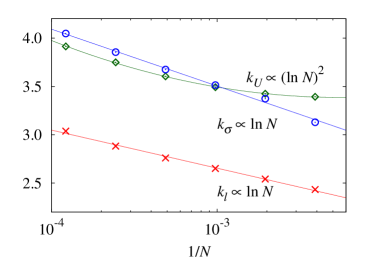
Figure 8: (Color online) The $N$-dependence of three specific values of $\langle k\rangle$: $k_{U}~{}\left(\diamond\right),\ k_{\sigma}\left(\circ\right),\ k_{l}~{}\left(\times\right)$. They are possible indicators of the disappearance of the left peak (see the main text for their precise definitions).

III.5 $P\left(l_{A}\right)$ in the thermodynamic limit

Finally, we return to the question posed early in this section: is the right peak the only lasting peak in the thermodynamic limit? To answer this question, we define possible indicators of the point at which the left peak becomes unobservable. The $N$-dependence of those indicators may reveal whether the left peak survives in the thermodynamic limit.

The curves shown in Fig. 7 reflect the $\langle k\rangle$-dependence of $P\left(l_{A}\right)$. As $\langle k\rangle$ grows, we observe the shift of the single (right) peak to the right, and then the formation of the left peak, and finally the increasing inter-peak separation with the dominance of the left peak, as Fig. 3(a) illustrates. This produces the single-peaked curves as shown in Fig. 7(a). Although not exhibited here, $\left[\langle l_{A}\rangle\right]$ shows a similar behavior. Meanwhile, the Binder cumulant $U_{4}$ indicates the separation between two peaks, whose value decreases far below zero as the separation increases indefinitely with $\langle k\rangle$.

To investigate the finite-size scaling of Fig. 7, we define the three specific values of $\langle k\rangle$ as

• $k_{U}$: the largest $\langle k\rangle$ that satisfies $U_{4}=0$,

• $k_{\sigma}$: the location of $\max\sigma^{2}$,

• $k_{l}$: the location of $\max\left[\langle l_{A}\rangle\right]$.

Taking those three points as possible indicators of the critical value of $\langle k\rangle$ at which the left peak is barely observable, we observe that all the three values increases indefinitely with $N$ (see Fig. 8). This implies that as $N$ goes to infinity, the $l_{A}$ distribution is single-peaked at any finite $\langle k\rangle$, and that the peak is far away (as it is actually the “right” peak) from $l_{A}=0$. Hence, this observation again supports our previous claim that the right peak is actually the only lasting peak in the thermodynamic limit.

IV Summary and Discussions

In summary, we have studied the absorbing states of zero-temperature Glauber dynamics in quenched ER-type random networks with zero-magnetization initial states. Each absorbing state has been represented by its active link density $l_{A}$. We have found that the structure of the $l_{A}$ distribution consists of two self-averaging peaks, the left one with samples almost reaching the ground state and the right one with samples divided by large stable domain walls. The mean of the left-peak (right-peak) component seems to be a monotonically decreasing (increasing) function of $\langle k\rangle$. In particular, we focus on the finite-size scaling analysis of various physical properties for $P(l_{A})$, which suggests that the fraction of the right-peak component stays finite in the thermodynamic limit, even if the value of $\langle k\rangle$ is pretty high. We have also gathered circumstantial evidence that the right peak is actually the only lasting peak in the thermodynamic limit.

Our results also have some implications on opinion dynamics studies. Some earlier studies of zero-temperature Glauber dynamics as an opinion dynamics model have simply assumed that when there are sufficiently many links, the portion of samples that do not reach the ground state becomes negligible. Thus, they measured “consensus time,” which is the time required for the sample to reach the ground state in order to obtain the scaling relationship between the system size and the speed of relaxation. We suggest that consensus time is not a suitable measure since almost all the samples fail to reach the ground state in the thermodynamic limit and increasingly many of them end up far away from the ground state as $\langle k\rangle$ gets larger ODComment . Data collapse shown in Fig. 2 (the results of Castellano2005 as well) is a better numerical approach to such a problem. The final location of the right peak is very well-defined and it seems to represent the only value of $l_{A}$ that yields stable up-down symmetric configurations. Therefore, interfacial noise that causes sufficiently large fluctuations in $l_{A}$ always drives the system out of absorbing states and helps them relax to the ground state, as illustrated by the role played by blinkers in even-degree regular random networks. This leads us to expect that there should be an analytical argument for the location of the right peak, which we unfortunately could not formulate. As the right peak observed in odd-degree regular random networks shows a qualitatively similar behavior, an intuitive argument for the nature of the right peak in one substrate may help us understand the corresponding phenomenon in the other substrate.

Finally, we have shown that the properties of $P(l_{A})$ are not much affected by either the particular network structure or initial configuration, where both peaks can be reached purely from the stochasticity of dynamics. This may be due to the characteristic homogeneity of ER networks, as any randomly generated ER network in any randomly chosen symmetric initial configurations is likely to be very similar to another ER network prepared in the same way. It would be interesting to check whether the same observation can be made for more topologically heterogeneous substrates such as scale-free networks. One should note that this argument for the “irrelevance of structure and configuration” should be taken carefully. As Uchida and Shirayama have shown Uchida2007 , the biased choice of initial configuration does affect the properties of $P(l_{A})$. The contributions from such exceptional cases are negligible in the unbiased ensemble of samples we have considered in this paper.

References

- (1) R. J. Glauber, J. Math. Phys. 4, 294 (1963).
- (2) V. Spirin, P. L. Krapivsky, and S. Redner, Phys. Rev. E 63, 036118 (2001); K. Barros, P. L. Krapivsky, and S. Redner, ibid. 80, 040101 (2009).
- (3) V. Spirin, P. L. Krapivsky, and S. Redner , Phys. Rev. E 65, 016119 (2001).
- (4) J. Olejarz, P. L. Krapivsky, and S. Redner, Phys. Rev. E 83, 030104 (2011).
- (5) P. Svenson, Phys. Rev. E 64, 036122 (2001).
- (6) C. Castellano, V. Loreto, A. Barrat, F. Cecconi, and D. Parisi, Phys. Rev. E 71, 066107 (2005).
- (7) H. Zhou and R. Lipowsky, Proc. Natl. Acad. Sci. 102, 10052 (2005); H. Zhou and R. Lipowsky, J. Stat. Mech. (2007) P01009; C. Castellano and R. Pastor-Satorras, ibid.. P05001 (2006); C. P. Herrero, J. Phys. A: Math. Theor. 42, 415102 (2009).
- (8) O. Häggström, Physica A 310, 275 (2002).
- (9) M. Uchida and S. Shirayama, Phys. Rev. E 75, 046105 (2007).
- (10) P. Erdős and A. Rényi, Publicationes Mathematicae (Debrecen), Vol. 6 (1959), pp. 290-297; E. N. Gilbert, Ann. Math. Stat. 30, 1141 (1959).
- (11) While Svenson2001 uses the original definition of the ER networks, Castellano2005 imposes a constraint that most of the system belongs to the same component. While the former is concerned about the shape of the absorbing states, the latter is concerned more about the system size dependence of consensus time, where knowledge about the size of each connected component is more important. Our study is more in the spirit of Svenson2001 , so we do not impose any constraints on the connectedness of the system.
- (12) Note that opinion dynamics models deal with single-component systems. Our study is about the ER network, which is naturally composed of multiple components. One should bear this difference in mind when interpreting our results. Still, we can safely say that our argument against the concept of consensus time generalizes to connected systems. At large values of , the giant component’s contribution to is overwhelmingy large. Therefore, if the whole network is stuck far away from the ground state, so is the giant component.