Semi-quantum molecular dynamics simulation of thermal properties and heat transport in low-dimensional nanostructures

Abstract

We present a detailed description of semi-quantum molecular dynamics simulation of stochastic dynamics of a system of interacting particles. Within this approach, the dynamics of the system is described with the use of classical Newtonian equations of motion in which the effects of phonon quantum statistics are introduced through random Langevin-like forces with a specific power spectral density (the color noise). The color noise describes the interaction of the molecular system with the thermostat. We apply this technique to the simulation of thermal properties and heat transport in different low-dimensional nanostructures. We describe the determination of temperature in quantum lattice systems, to which the equipartition limit is not applied. We show that one can determine the temperature of such system from the measured power spectrum and temperature- and relaxation-rate-independent density of vibrational (phonon) states. We simulate the specific heat and heat transport in carbon nanotubes, as well as the heat transport in molecular nanoribbons with perfect (atomically smooth) and rough (porous) edges, and in nanoribbons with strongly anharmonic periodic interatomic potentials. We show that the effects of quantum statistics of phonons are essential for the carbon nanotube in the whole temperature range $T<500$K, in which the values of the specific heat and thermal conductivity of the nanotube are considerably less than that obtained within the description based on classical statistics of phonons. This conclusion is also applicable to other carbon-based materials and systems with high Debye temperature like graphene, graphene nanoribbons, fullerene, diamond, diamond nanowires etc. We show that the existence of rough edges and quantum statistics of phonons change drastically the low temperature thermal conductivity of the nanoribbon in comparison with that of the nanoribbon with perfect edges and classical phonon dynamics and statistics. The semi-quantum molecular dynamics approach allows us to model the transition in the rough-edge nanoribbons from the thermal-insulator-like behavior at high temperature, when the thermal conductivity decreases with the conductor length, to the ballistic-conductor-like behavior at low temperature, when the thermal conductivity increases with the conductor length. We also show how the combination of strong nonlinearity of periodic interatomic potentials with the quantum statistics of phonons changes completely the low-temperature thermal conductivity of the system.

I Introduction

Molecular dynamics (MD) is a method of numerical modeling of molecular systems based on classical Newtonian mechanics. It does not allow for the description of pure quantum effects such as freezing out of high-frequency oscillations at low temperatures and the related decrease to zero of heat capacity for $T\rightarrow 0$. In classical molecular dynamics (CMD), each dynamical degree of freedom possesses the same energy $k_{B}T$, where $k_{B}$ is Boltzmann constant. Therefore, in classical statistics the specific heat of a solid almost does not depend on temperature when only relatively small changes, caused the anharmonicity of the potential, can be taken into account landau1 . On the other hand, because of its complexity, a pure quantum-mechanical description does not allow in general the detailed modeling of the dynamics of many-body systems. To overcome these obstacles, different semiclassical methods, which allow to take into an account quantum effects in the dynamics of molecular systems, have been proposed wang ; donadio ; heatwole ; buyukdagli ; ceriotti ; dammak ; wang2 . The most convenient for the numerical modeling is the use of the Langevin equations with color-noise random forces buyukdagli ; dammak . In this approximation, the dynamics of the system is described with the use of classical Newtonian equations of motion, while the quantum effects are introduced through random Langevin-like forces with a specific power spectral density (the color noise), which describe the interaction of the molecular system with the thermostat. Below we give a detailed description of this semi-quantum molecular dynamics (SQMD) approach in application to the simulation of specific heat and heat transport in different low-dimensional nanostructures.

The paper is organized as follows. In Section II we describe the temperature-dependent Langevin dynamics of the system under the action of random forces. If the random forces are delta-correlated in time domain, this corresponds to the white noise with a flat power spectral density. This situation corresponds to high enough temperatures, when $k_{B}T$ is larger that the quantum of the highest-frequency mode in the system, $k_{B}T\gg\hbar\omega_{m}$. But for low enough temperature, $k_{B}T\ll\hbar\omega_{m}$, the stochastic dynamics of the system should be described with the use of random Langevin-like forces with a non-flat power spectral density, which corresponds to the system with color noise. In Section III we describe the determination of temperature in quantum lattice systems, to which the equipartition limit is not applied. We show how one can determine the temperature of such system from the measured power spectrum and temperature- and relaxation-rate-independent density of vibrational (phonon) states. In Section IV we describe a method for the generation of color noise with the power spectrum, which is consistent with the quantum fluctuation-dissipation theorem landau1 ; callen . In Sections V and VII we apply such semi-quantum molecular dynamics approach to the simulation of the specific heat and phonon heat transport in carbon nanotubes. In Section VI we apply this method to the simulation of heat transport in a molecular nanoribbon with rough edges. Previously, we have predicted analytically kosevich1 and confirmed by classical molecular dynamics simulations kosevich2 that rough edges of molecular nanoribbon (or nanowire) cause strong suppression of phonon thermal conductivity due to strong momentum-nonconserving phonon scattering. Here we show that the rough edges and quantum statistics of phonons change drastically the thermal conductivity of the rough-edge nanoribbon in comparison with that of the nanoribbon with perfect (atomically smooth) edges. The semi-quantum molecular dynamics approach allows us to model the transition in the rough-edge nanoribbons from the thermal-insulator-like behavior at high temperature, when the thermal conductivity decreases with the conductor length, see Ref. kosevich2 , to the ballistic-conductor-like behavior at low temperature, when the thermal conductivity increases with the conductor length. In Section VIII we apply this technique to the simulation of thermal transport in a nanoribbon with strongly anharmonic periodic interatomic potentials. We show how the combination of strong nonlinearity of the interatomic potentials with quantum statistics of phonons changes completely the low-temperature thermal conductivity of the nanoribbon. In Section IX we provide a summary and discussions of all the main results of the paper.

II Langevin equations with color noise

In the presence of a Langevin thermostat, equations of motion of coupled particles have the following form:

$$M_{n}\ddot{\rm\bf r}_{n}=-\frac{\partial}{\partial{\rm\bf r}_{n}}H-M_{n}\Gamma\dot{\rm\bf r}_{n}+{\Xi}_{n},$$ (1)

where the three-dimensional radius-vector ${\rm\bf r}_{n}(t)$ gives the position of the $n$-th particle at the time instant $t$ ($n=1,2,\dots,N$, $N$ being the total number of particles), $M_{n}$ is the particle mass, $H$ is the Hamiltonian of the system and ${\rm\bf F}_{n}=-\partial H/\partial{\rm\bf r}_{n}$ gives the force applied to the $n$-th particle caused by the interaction with the other particles, $\Gamma=1/t_{r}$ is the friction coefficient ($t_{r}$ being the relaxation time due to the interaction with the thermostat), and $\Xi_{n}=\{\xi_{\alpha,n}\}_{\alpha=1}^{3}$ are random forces with the Gaussian distribution.

In the semi-quantum approach the random forces do not represent in general white noise. The power spectral density of the random forces in that description should be given by the quantum fluctuation-dissipation theorem landau1 ; callen :

$$\langle\xi_{\alpha n}\xi_{\beta m}\rangle_{\omega}=2M_{n}\Gamma k_{B}T\delta_{\alpha\beta}\delta_{nm}p(\omega,T),$$ (2)

where $n,m=1,2,...,N$, $\alpha,\beta=1,2,3$ are Cartesian components, $\delta_{nm}$ and $\delta_{\alpha\beta}$ are Kronecker delta-symbols. Here the positive and even in frequency $\omega$ function

$$p(\omega,T)=\frac{1}{2}\frac{\hbar\omega}{k_{B}T}+\frac{\hbar\omega/k_{B}T}{\exp(\hbar\omega/k_{B}T)-1}$$ (3)

$$=\frac{\hbar\omega}{2k_{B}T}\coth(\frac{\hbar\omega}{2k_{B}T})$$

gives the dimensionless power spectral density at temperature $T$ of an oscillator with frequency $\omega$. The first term in Eq. (3) gives the contribution of the zero-point oscillations to the power spectral density of random forces. With the use of Eqs. (2) and (3), we get the correlation function of the random forces as

$$\langle\xi_{\alpha n}(t)\xi_{\beta m}(0)\rangle=\int_{-\infty}^{+\infty}\langle\xi_{\alpha n}\xi_{\beta m}\rangle_{\omega}e^{i\omega t}\frac{d\omega}{2\pi}$$

$$=2M_{n}\Gamma k_{B}T\delta_{\alpha\beta}\delta_{nm}\int_{-\infty}^{+\infty}p(\omega,T)e^{i\omega t}\frac{d\omega}{2\pi}~{}.$$ (4)

Let $\Omega_{max}$ be the maximal vibrational eigenfrequency of the molecular system. At high temperatures, $T\gg\hbar\Omega_{max}/k_{B}$, one has $p(\omega,T)=1$ and the molecular system will perceive the random forces as a delta-correlated white noise:

$$\langle\xi_{\alpha n}(t)\xi_{\beta m}(0)\rangle=2M_{n}\Gamma k_{B}T\delta_{\alpha\beta}\delta_{nm}\delta(t).$$ (5)

Therefore for high enough temperatures we deal with molecular dynamics with Langevin uncorrelated random forces. But for low temperatures, the random forces are correlated according to the function given by Eqs. (3) and (4). In other words, for low temperatures the random forces in the system represent the color noise with the dimensionless power spectral density $p(\omega,T)$ given by Eq. (3).

III Determination of temperature in quantum lattice systems

In connection with the consideration of the thermodynamics and dynamics of non-classical lattices, in this Section we discuss possible determination of the temperature in the systems, to which the equipartition limit is not applied. We start from Eqs. (1), rewritten as the equations of motion for the lattice vibrational mode with eigenfrequency $\Omega_{n}$:

$$M_{n}\ddot{\rm\bf Q}_{n}+M_{n}\Gamma\dot{\rm\bf Q}_{n}+M_{n}\Omega^{2}_{n}{\rm\bf Q}_{n}={\Xi}_{n},$$ (6)

where $\Xi_{n}=\{\xi_{\alpha,n}\}_{\alpha=1}^{3}$ are random forces with the spectral density given by Eqs. (2) and (3).

From Eqs. (2), (3) and (6) we obtain

$$M_{n}\langle Q^{2}_{n}\rangle_{\omega,T}=\frac{\hbar\omega}{2}\coth(\frac{\hbar\omega}{2k_{B}T})\frac{2\Gamma}{(\Omega^{2}_{n}-\omega^{2})^{2}+\omega^{2}\Gamma^{2}},$$ (7)

and power spectrum $\tilde{E}_{T}(\omega)$ of lattice vibrations with $3N-6$ nonzero eigenmodes:

$$\tilde{E}_{T}(\omega)=\sum_{n=7}^{3N}\frac{1}{2}M_{n}(\omega^{2}+\Omega_{n}^{2})\langle Q^{2}_{n}\rangle_{\omega,T}$$

$$=\sum_{n=7}^{3N}M_{n}\omega^{2}\langle Q^{2}_{n}\rangle_{\omega,T}=\sum_{n=7}^{3N}M_{n}\Omega_{n}^{2}\langle Q^{2}_{n}\rangle_{\omega,T}$$

$$=\frac{\hbar\omega}{2}\coth(\frac{\hbar\omega}{2k_{B}T})\sum_{n=7}^{3N}\frac{\Gamma(\omega^{2}+\Omega_{n}^{2})}{(\Omega^{2}_{n}-\omega^{2})^{2}+\omega^{2}\Gamma^{2}}$$

$$=\frac{\hbar\omega}{2}\coth(\frac{\hbar\omega}{2k_{B}T})\sum_{n=7}^{3N}\frac{2\Gamma\omega^{2}}{(\Omega^{2}_{n}-\omega^{2})^{2}+\omega^{2}\Gamma^{2}}$$

$$=\frac{\hbar\omega}{2}\coth(\frac{\hbar\omega}{2k_{B}T})\sum_{n=7}^{3N}\frac{2\Gamma\Omega_{n}^{2}}{(\Omega^{2}_{n}-\omega^{2})^{2}+\omega^{2}\Gamma^{2}}.$$ (8)

We can use $\langle Q^{2}_{n}\rangle_{\omega,T}$ and the power spectrum $\tilde{E}_{T}(\omega)$, Eqs. (7) and (8), to compute the average energy of the system. Taking into account that the above quantities are even functions of frequency $\omega$, for positive $\omega$ the average energy of the system can be computed as:

$$E(T)=\int_{-\infty}^{\infty}\tilde{E}_{T}(\omega)\frac{d\omega}{2\pi}=\int_{0}^{\infty}\tilde{E}_{T}(\omega)\frac{d\omega}{\pi}.$$ (9)

In the weakly dissipative limit, with $\Gamma\ll\Omega_{n}$ for all $\Omega_{n}$, which is realized in all the considered system, for positive $\omega$ and $\Omega_{n}$ one has, in the sense of generalized functions:

$$\frac{2\Gamma\omega^{2}}{(\Omega^{2}_{n}-\omega^{2})^{2}+\omega^{2}\Gamma^{2}}\approx\frac{2\Gamma\Omega_{n}^{2}}{(\Omega^{2}_{n}-\omega^{2})^{2}+\omega^{2}\Gamma^{2}}$$

$$\approx \frac{\Gamma(\Omega_{n}^{2}+\omega^{2})}{(\Omega^{2}_{n}-\omega^{2})^{2}+\omega^{2}\Gamma^{2}}\approx\pi\delta(\omega-\Omega_{n}).$$ (10)

We can introduce in this limit the density of vibrational (phonon) states (for positive frequencies) as:

$$D(\omega)=\sum_{n=7}^{3N}\frac{2\Gamma\Omega_{n}^{2}}{(\Omega^{2}_{n}-\omega^{2})^{2}+\omega^{2}\Gamma^{2}}\approx\pi\sum_{n=7}^{3N}\delta(\omega-\Omega_{n}).$$ (11)

Then the power spectrum (for positive $\omega$) consists of an array of the delta-functions at the system eigenfrequencies, weighted by temperature,

$$\tilde{E}_{T}(\omega) \equiv \frac{\hbar\omega}{2}\coth(\frac{\hbar\omega}{2k_{B}T})D(\omega)$$ (12)

$$= \frac{\pi}{2}\hbar\omega\coth(\frac{\hbar\omega}{2k_{B}T})\sum_{n=7}^{3N}\delta(\omega-\Omega_{n}),$$

and the average energy of the system (9) has the following form:

$$E(T)=\sum_{n=7}^{3N}\left[\frac{1}{2}\hbar\Omega_{n}+\frac{\hbar\Omega_{n}}{\exp(\hbar\Omega_{n}/k_{B}T)-1}\right].$$ (13)

Here the first term in the sum gives the temperature-independent contribution of zero-point oscillations to the energy of the system. As one can see from Eqs. (11)-(13), in the weakly dissipative limit the density of vibrational states, power spectrum and average energy of the system do not depend explicitly on the relaxation rate $\Gamma$.

From Eq. (12) we get the ”quantum definition”  of temperature $T$ through the power spectrum of lattice vibrations at the given frequency:

$$T=\hbar\omega/\left(k_{B}\ln\left[\frac{1+A_{T}(\omega)}{1-A_{T}(\omega)}\right]\right),$$ (14)

where

$$A_{T}(\omega)=\hbar\omega D(\omega)/(2\tilde{E}_{T}(\omega)).$$ (15)

In the case when one omits the zero-point contribution to the spectrum of the random forces, namely considers

$$p(\omega,T)=\frac{\hbar\omega/k_{B}T}{\exp(\hbar\omega/k_{B}T)-1}$$ (16)

in Eqs. (2) and (6), the temperature can be determined from the following equation:

$$T=\hbar\omega/(k_{B}\ln\left[1+2A_{T}(\omega)\right]),$$ (17)

where in the definition of the function $A_{T}(\omega)$ in Eq. (15) the function $\tilde{E}_{T}(\omega)$, in contrast to function $\tilde{E}_{T}(\omega)$ in Eq. (8), does not have now the zero-point contribution,

$$\tilde{E}_{T}(\omega)=\frac{\hbar\omega}{\exp(\hbar\omega/k_{B}T)-1}\sum_{n=7}^{3N}\frac{2\Gamma\Omega_{n}^{2}}{(\Omega^{2}_{n}-\omega^{2})^{2}+\omega^{2}\Gamma^{2}},$$ (18)

and, correspondingly, one has

$$E(T)=\sum_{n=7}^{3N}\frac{\hbar\Omega_{n}}{\exp(\hbar\Omega_{n}/k_{B}T)-1}.$$ (19)

In the equipartition limit, which is realized for $T\gg\hbar\Omega_{max}/k_{B}$, one has $\tilde{E}_{T}(\omega)=k_{B}TD(\omega)$, $A_{T}(\omega)\ll 1$, and both Eqs. (14) and (17) turn into the identity $T=T$.

Therefore one can determine the temperature of the quantum lattice system from the measured power spectrum $\tilde{E}_{T}(\omega)$ and temperature- and relaxation-rate-independent density of vibrational (phonon) states $D(\omega)$. In Fig. 6 we show the power spectrum, computed within the semi-quantum approach with $\Gamma=1/t_{r}$, $t_{r}=0.4$ ps, line 1, and in the limit, when the spectrum is given by an array of the smoothed delta-functions, line 3. As one can see in this figure, the particular choice of the (long enough) relaxation time $t_{r}=1/\Gamma$ indeed does not affect the presented results. The determination of temperature, given by Eqs. (14) and (17), is valid for weakly anharmonic systems, in which the power spectrum of lattice vibrations is close to the one, given by Eq. (8). Carbon-based materials like carbon nanotubes, graphene and graphene nanoribbons, and crystal structures with stiff valence bonds belong to such systems. It is worth mentioning that the temperature, given by Eq. (14) or Eq. (17), does not depend on frequency $\omega$ only in the case of equilibrium harmonic lattice excitations, driven by random forces with power spectrum given by the Bose-Einstein distribution, Eqs. (2) and (3). The anharmonicity of the lattice can change the power spectrum of the excitations, see Fig. 12 (b) below. In such case the ”phonon temperature”  starts to depend on frequency (similar to the frequency- and direction-dependent temperature of photons in non-equilibrium radiation, see Ref. landau1 ), and ”hot phonons”  with non-equilibrium high frequencies appear in the system, see Section VI below.

IV Color noise generation

For the implementation of the semi-quantum approach in molecular dynamics, random forces with the power spectral density given by $p(\bar{\omega})$ must be generated. Existing numerical techniques allow the generation of a random quantity from a prescribed correlation function maradu . This approximation was used in dammak in the modeling of thermodynamic properties of liquid ⁴He above the $\lambda$ point. But universal methods require in general the usage of high numerical resources. For instance, the utilization of the method proposed in maradu requires the execution of the Fast Fourier Transform for every random force value. We propose a technique which takes into account the specific form of the dimensionless power spectral density $p(\bar{\omega})$, where $\bar{\omega}=\hbar\omega/k_{B}T$ is a dimensionless frequency.

In terms of $\bar{\omega}$, the dimensionless power spectral density of random forces looks as

$$p(\bar{\omega})=\frac{1}{2}\bar{\omega}+\frac{\bar{\omega}}{\exp(\bar{\omega})-1}=\frac{1}{2}{\bar{\omega}}\coth(\bar{\omega}/2).$$ (20)

The random force with dimensionless power spectral density, given by Eq. (20), can be presented as a sum of two independent functions, $p(\bar{\omega})=p_{0}(\bar{\omega})+p_{1}(\bar{\omega})$, where the first function, $p_{0}(\bar{\omega})=\bar{\omega}/2$, has a linear power spectral density, while the second one is $p_{1}(\bar{\omega})=\bar{\omega}/[\exp(\bar{\omega})-1]$.

To generate the color noise with a given dimensionless power spectral density $p(\bar{\omega})$, we will construct the dimensionless random vector functions ${\bf\rm S}_{n}(\tau)=\{S_{\alpha,n}\}_{\alpha=1}^{3}={\bf\rm S}_{0n}(\tau)+{\bf\rm S}_{1n}(\tau)$ of the dimensionless time $\tau=tk_{B}T/\hbar$, which will give the power spectral density of the random forces in Eqs. (1) as

$$\langle\xi_{\alpha n}\xi_{\beta m}\rangle_{\omega}=2M_{n}\Gamma k_{B}T\langle S_{\alpha n}S_{\beta m}\rangle_{\bar{\omega}},$$ (21)

such that

$$\langle\xi_{\alpha n}(t)\xi_{\beta m}(0)\rangle=\int_{-\infty}^{+\infty}\langle\xi_{\alpha n}\xi_{\beta m}\rangle_{\omega}e^{i\omega t}\frac{d\omega}{2\pi}$$

$$=2M_{n}\Gamma k_{B}T\int_{-\infty}^{+\infty}\langle S_{\alpha n}S_{\beta m}\rangle_{\bar{\omega}}e^{i\omega t}\frac{d\omega}{2\pi}$$

$$=\frac{2}{\hbar}M_{n}\Gamma(k_{B}T)^{2}\int_{-\infty}^{+\infty}\langle S_{\alpha n}S_{\beta m}\rangle_{\bar{\omega}}e^{i\bar{\omega}\tau}\frac{d\bar{\omega}}{2\pi}~{},$$ (22)

and

$$\langle S_{\alpha n}S_{\beta m}\rangle_{\bar{\omega}}=\langle S_{0\alpha n}S_{0\beta m}\rangle_{\bar{\omega}}+\langle S_{1\alpha n}S_{1\beta m}\rangle_{\bar{\omega}}.$$ (23)

Here, the uncorrelated random functions ${\bf\rm S}_{0n}(\tau)$ and ${\bf\rm S}_{1n}(\tau)$ will generate, in a finite frequency interval, the power spectra $p_{0}(\bar{\omega})$ and $p_{1}(\bar{\omega})$, respectively.

For a molecular system with maximal vibrational eigenfrequency $\omega_{m}$, we will construct the dimensionless random vector function ${\bf\rm S}_{0n}(\tau)$, whose power spectral density generates $p_{0}(\bar{\omega})$ in the frequency interval $[0,\bar{\omega}_{m}]$ ($\bar{\omega}_{m}=\hbar\omega_{m}/k_{B}T$). Each component of this vector can be written as a sum of dimensionless random functions

$$S_{0\alpha n}(\tau)=\sum_{i=1}^{4}c_{i}[\eta_{\alpha n,i}(\tau)-\zeta_{\alpha n,i}(\tau)].$$ (24)

The functions $\{\zeta_{\alpha ni}\}_{i=1}^{4}$ which generate the color noise, are the solutions of the linear equations:

$$\zeta^{\prime}_{\alpha ni}(\tau)=\lambda_{i}[\eta_{\alpha ni}(\tau)-\zeta_{\alpha ni}(\tau)],$$ (25)

where $\zeta^{\prime}_{\alpha ni}(\tau)$ is the derivative with respect to $\tau$. Here $\eta_{\alpha ni}(\tau)$ are dimensionless white-noise random forces, with the correlation functions

$$\langle\eta_{\alpha ni}(\tau)\eta_{\beta kj}(0)\rangle=2\delta_{\alpha\beta}\delta_{nk}\delta_{ij}\delta(\tau)/\lambda_{i}.$$ (26)

By solving Eqs. (25) in the frequency domain, $\zeta_{\alpha ni}$ can be substituted in Eq. (24) and the power spectra of ${\rm\bf S}_{0n}$ can be obtained as

$$\langle S_{0\alpha n}S_{0\beta m}\rangle_{\bar{\omega}}=\delta_{\alpha\beta}\delta_{mn}\sum_{i=1}^{4}\frac{2c_{i}^{2}\bar{\omega}^{2}}{\lambda_{i}(\lambda_{i}^{2}+\bar{\omega}^{2})}.$$ (27)

The dimensionless parameters $c_{i}$ and $\lambda_{i}$ can be found by minimizing the integral

$$\int_{0}^{1}\left[\frac{1}{2}x-\sum_{i=1}^{4}\frac{2\bar{c}_{i}^{2}x^{2}}{\bar{\lambda}_{i}(\bar{\lambda}_{i}^{2}+x^{2})}\right]^{2}dx$$ (28)

with respect to the parameters $\bar{c}_{1},\bar{\lambda}_{1},...,\bar{c}_{4},\bar{\lambda}_{4}$, where $\bar{c}_{i}=c_{i}/\bar{\omega}_{m}$, $\bar{\lambda}_{i}=\lambda_{i}/\bar{\omega}_{m}$. The coefficients $c_{i}$, $\lambda_{i}$, $i=1,...,4$, obtained within this procedure, are shown in Table 1. For these parameters, integral (28) reaches its lower value, equal to $2.46\times 10^{-8}$.

Table 1: Value of the coefficients $\lambda_{i}$, $c_{i}$, $\bar{\Omega}_{i}$, $\bar{\Gamma}_{i}$.

coefficient	value	coefficient	value
$\lambda_{1}/\bar{\omega}_{m}$	1.763817	$c_{5}$	1.8315
$\lambda_{2}/\bar{\omega}_{m}$	0.394613	$c_{6}$	0.3429
$\lambda_{3}/\bar{\omega}_{m}$	0.103506	$\bar{\Omega}_{5}$	2.7189
$\lambda_{4}/\bar{\omega}_{m}$	0.015873	$\bar{\Omega}_{6}$	1.2223
$c_{1}/\bar{\omega}_{m}$	1.043576	$\bar{\Gamma}_{5}$	5.0142
$c_{2}/\bar{\omega}_{m}$	0.177222	$\bar{\Gamma}_{6}$	3.2974
$c_{3}/\bar{\omega}_{m}$	0.050319
$c_{4}/\bar{\omega}_{m}$	0.010241

As one can see from Fig. 1, the function given by Eq. (27) approximates with high accuracy the linear function $p_{0}(\bar{\omega})=\bar{\omega}/2$ in the frequency interval $0.015\leq\bar{\omega}/\bar{\omega}_{m}<1.1$.

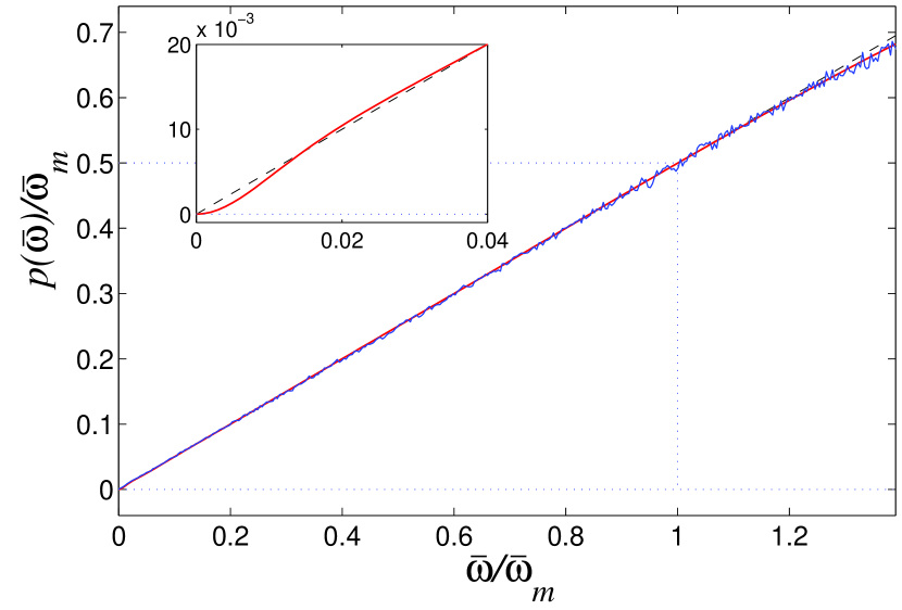
Figure 1: (Color online) Power spectral density of color noise $S_{0}(\tau)$ (blue line). Red line is given by Eq. (27), dashed line shows the linear function $p_{0}(\bar{\omega})/\bar{\omega}_{m}=\bar{\omega}/2\bar{\omega}_{m}$. The two lines practically coincide in the frequency interval $0.015\leq\bar{\omega}/\bar{\omega}_{m}\leq 1.1$. The inset shows spectral densities given by Eq. (27) (red line) and by linear function $p_{0}(\bar{\omega})/\bar{\omega}_{m}$ (dashed line) in the frequency interval $0\leq\bar{\omega}/\bar{\omega}_{m}\leq 0.04$. For color noise generation, Eqs. (25) were numerically integrated with the use of fourth order Runge-Kutta method with a constant integration step $\Delta\tau=0.05/\bar{\omega}_{m}$.

On the other hand, the random function $S_{1\alpha n}(\tau)$, which will generate the power spectral density $p_{1}(\bar{\omega})$, can be approximated by a sum of two random functions with relatively narrow frequency spectra:

$$S_{1\alpha n}(\tau)=c_{5}\zeta_{\alpha n5}(\tau)+c_{6}\zeta_{\alpha n6}(\tau).$$ (29)

In this sum the dimensionless random functions $\zeta_{\alpha ni}(\tau)$, $i=5,6$, satisfy the equations of motion as

$$\zeta^{\prime\prime}_{\alpha ni}(\tau)=\eta_{\alpha ni}(\tau)-\bar{\Omega}_{i}^{2}\zeta_{\alpha ni}(\tau)-\bar{\Gamma}_{i}\zeta^{\prime}_{\alpha ni}(\tau),$$ (30)

where, as before, $\eta_{\alpha ni}(\tau)$ are delta-correlated white noise functions:

$$\langle\eta_{\alpha ni}(\tau)\eta_{\beta kj}(0)\rangle=2\bar{\Gamma}_{i}\delta_{\alpha\beta}\delta_{nk}\delta_{ij}\delta(\tau).$$ (31)

We can solve, as previously, Eq. (30) in the frequency domain and insert $\zeta_{\alpha ni}$ into Eq. (29) to obtain the power spectrum of $S_{1\alpha n}$:

$$\langle S_{1\alpha n}S_{1\beta m}\rangle_{\bar{\omega}}=\delta_{\alpha\beta}\delta_{mn}\sum_{i=5}^{6}\frac{2c_{i}^{2}\bar{\Gamma}_{i}}{(\bar{\Omega}_{i}^{2}-\bar{\omega}^{2})^{2}+\bar{\omega}^{2}\bar{\Gamma}_{i}^{2}}$$ (32)

The dimensionless parameters $\{c_{i},\bar{\Omega}_{i},\bar{\Gamma}_{i}\}_{i=5}^{6}$ can be found by minimizing the integral

$$\int_{0}^{\infty}\left[\frac{\bar{\omega}}{\exp(\bar{\omega})-1}-\sum_{i=5}^{6}\frac{2c_{i}^{2}\bar{\Gamma}_{i}}{(\bar{\Omega}_{i}^{2}-\bar{\omega}^{2})^{2}+\bar{\omega}^{2}\bar{\Gamma}_{i}^{2}}\right]^{2}d\bar{\omega}$$ (33)

with respect to the parameters $c_{5},\bar{\Gamma}_{5},\bar{\Omega}_{5},c_{6},\bar{\Gamma}_{6},\bar{\Omega}_{6}$. The obtained parameters are shown in Table 1. For these parameters, integral (33) reaches its lower value, equal to $2.3\times 10^{-4}$. Since the integral (33) is determined by the rapid-descending functions, the infinite integration limit $[0,\infty)$ can be replaced by a finite one $[0,\bar{\omega}_{m}]$. Numerical integration of the integral (33) shows that its minimal value practically does not depend on the upper integration limit for $\bar{\omega}_{m}>20$.

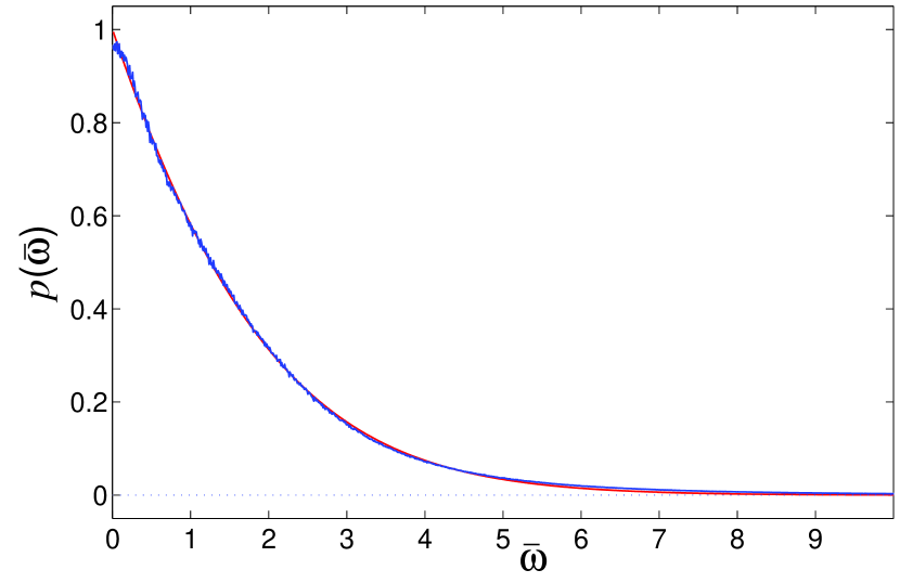
Figure 2: (Color online) Power spectral density of color noise $S_{1}(\tau)$, Eq. (32) (blue line). Red line shows the function $p_{1}(\bar{\omega})=\bar{\omega}/[\exp(\bar{\omega})-1]$. For color noise generation, Eqs. (30) were numerically integrated with the use of fourth order Runge-Kutta method with a constant integration step $\Delta\tau=0.02$.

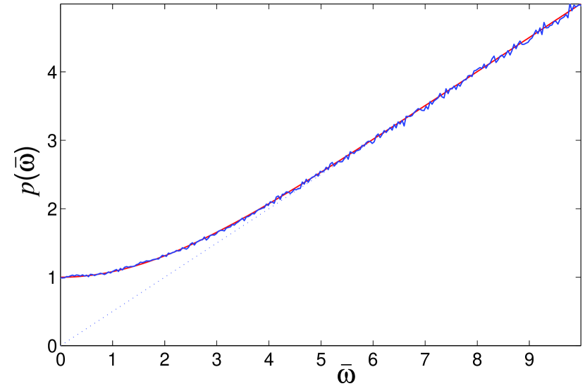
Figure 3: (Color online) Power spectral density of color noise $S_{0}(\tau)+S_{1}(\tau)$, given by the sum of Eqs. (27) and (32) (blue line). Red line shows the function $p(\bar{\omega})=(\bar{\omega}/2)\coth(\bar{\omega}/2)$. For color noise generation, Eqs. (25) and (30) were numerically integrated with the use of fourth order Runge-Kutta method with a constant integration step $\Delta t=0.005$. Maximal dimensionless frequency $\bar{\omega}_{m}=10$.

As one can see from Fig. 2, the function, given by Eq. (32), approximates with high accuracy the function $p_{1}(\bar{\omega})=\bar{\omega}/[\exp(\bar{\omega})-1]$ in the frequency interval $0\leq\bar{\omega}\leq 10$.

Therefore in the semi-quantum molecular dynamics approach one has to solve the Langevin equations (1) with random forces $\Xi_{n}=\{\xi_{\alpha n}\}_{\alpha=1}^{3}$, whose power spectral density is determined as:

$$\langle\xi_{\alpha n}\xi_{\beta m}\rangle_{\omega}=2M_{n}\Gamma k_{B}T[\langle S_{0\alpha n}S_{0\beta m}\rangle_{\bar{\omega}}+\langle S_{1\alpha n}S_{1\beta m}\rangle_{\bar{\omega}}]$$

$$=2M_{n}\Gamma k_{B}T\delta_{\alpha\beta}\delta_{mn}\left[\sum_{i=1}^{4}\frac{2c_{i}^{2}\bar{\omega}^{2}}{\lambda_{i}(\lambda_{i}^{2}+\bar{\omega}^{2})}\right.$$

$$\left.+\sum_{i=5}^{6}\frac{2c_{i}^{2}\bar{\Gamma}_{i}}{(\bar{\Omega}_{i}^{2}-\bar{\omega}^{2})^{2}+\bar{\omega}^{2}\bar{\Gamma}_{i}^{2}}\right].~{}~{}~{}$$ (34)

From Eq. (22) we get the relation between the dimension $\xi_{\alpha n}(t)$ and dimensionless $S_{\alpha n}(\tau)$ random forces: $\xi_{\alpha n}(t)=\xi_{\alpha n}(\hbar\tau/k_{B}T)=k_{B}T\sqrt{2M_{n}\Gamma/\hbar}[S_{0\alpha n}(\tau)+S_{1\alpha n}(\tau)]$.

In Fig. 3 we show the comparison of the power spectral density for the dimensionless frequency $\bar{\omega}$, given by the sum of Eqs. (27) and (32), with the function $(\bar{\omega}/2)\coth(\bar{\omega}/2)$, Eq. (20). We see a very good coincidence in the frequency interval $[0,\bar{\omega}_{m}]$ for $\bar{\omega}_{m}=10$.

To describe the dynamics of molecular system with an account for quantum statistics of molecular vibrations but without an account for zero-point oscillations, one has to keep only the last two terms, with $i=5,6$, in Eq. (34) and to solve numerically Eqs. (30) in order to simulate random forces in Eq. (1). Equations (30) play the role of the filter, which filters out the dimensionless high-frequency (”non-quantum”) component of the white noise at low temperature.

It is worth mentioning in this connection that the considered semi-quantum approach permits one to obtain the correct value of the energy of zero-point oscillations. A semi-quantum account for zero-point oscillations in the modeling of the properties of liquid ⁴He above the $\lambda$ point has allowed to describe correctly the liquid state of the helium dammak , while the classical molecular dynamics description (without an account for zero-point oscillations) predicts the solid state of the helium at the same low temperature.

V Temperature dependence of specific heat of carbon nanotube

For the illustration of the implementation of the semi-quantum approach in molecular dynamics, in this Section we find the temperature dependence of specific heat of a single-walled carbon nanotube. We consider the nanotube with the (5,5) chirality index (the zig-zag structure), which consists of $N=300$ carbon atoms, see Fig. 4. In the following we will use the molecular-dynamics model of the carbon nanotube, which was discussed in details in Ref. savin1 .

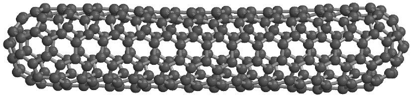
Figure 4: Form of a single-walled carbon nanotube C₃₀₀ with the zig-zag structure, which consists of $N=300$ carbon atoms.

To model nanotube dynamics at temperature $T$ in the classical approximation, we will solve the Langevin equation (1) with a white noise, where $H$ is a Hamiltonian of the nanotube and all $M_{n}\equiv M$, $M$ being a mass of a carbon atom. The correlation functions of the random forces $\Xi_{n}$, which describe the interaction of an $n$-th atom with the thermostat, are given by Eq. (5).

We take the initial conditions, which correspond to the equilibrium stationary state of the nanotube at $T=0$, and integrate a system of equations of motion (1) for the time $t=20t_{r}$, during which the system will reach the equilibrium state at finite temperature. The integration beyond this time will allow us to find the average thermal energy of the system $\langle H\rangle=E(T)$. Then the specific heat of the molecular system can be found from the temperature dependence of the average thermal energy $C(T)=dE(T)/dT$. As one can see in Fig. 5, the average thermal energy of the carbon nanotube, placed in classical Langevin thermostat, is strictly proportional to temperature, $E(T)=(3N-6)k_{B}T\approx 3Nk_{B}T$, line 1, and, correspondingly, nanotube specific heat almost does not depend on temperature, line 3. This result shows both the correctness of the modeling and that carbon nanotubes are stiff structures which possess weak anharmonicity of the dynamics of the constituting atoms. One can also see in Fig. 5 that the average thermal energy per mode $e(T)$ without an account for zero-point oscillations has the feature that $e(T)\leq k_{B}T$ in general and $e(T)\ll k_{B}T$ for temperature much less than the Debye one. For instance, in the carbon nanotube $e(T)$ is almost six times less than $k_{B}T$ at room temperature $T$=300 K.

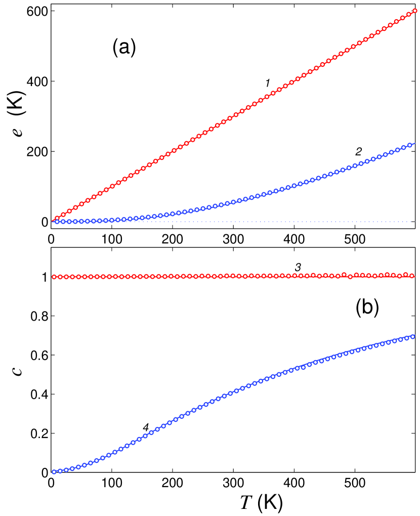
Figure 5: (Color online) Temperature dependence of the average thermal energy per mode $e=E/3Nk_{B}$ (a) and specific heat per mode $c=C/3Nk_{B}$ (b) of a single-walled carbon nanotube C₃₀₀. Lines 1 and 3 show the dependencies, obtained with classical Langevin thermostat, red circles give the result of numerical modeling. Lines 2 and 4 give the dependencies, obtained within the quantum description with the use of eigenmode spectra without an account for zero-point oscillations, Eqs. (19) and (35), blue circles give the result obtained within the semi-quantum molecular dynamics approach.

To obtain power spectra of the thermal oscillations of the atoms in the carbon nanotube, one has to switch off the interaction with the thermostat after the establishment of the thermal equilibrium in the system. In other words, one has to solve numerically the frictionless equations of motion, Eqs. (1) with $\Gamma=0$ and $\Xi_{n}={\rm\bf 0}$, with the initial conditions for ${\rm\bf r}_{n}$ and $\dot{\rm\bf r}_{n}$, which correspond to the thermalized state of the molecular system. By performing the Fast Fourier Transform of the time-dependent particle velocities $\dot{\rm\bf r}_{n}(t)$, one can get the power spectrum $\tilde{E}_{T}(\omega)$, Eq. (8). To increase the accuracy of the measurement, it is necessary to perform the averaging of the obtained results on different initial thermalized states of the system. Power spectral density of the thermal vibrations of the carbon nanotube atoms is shown in Fig. 6. As one can see from this figure, all vibrational modes of the system are excited in the classical Langevin thermostat.

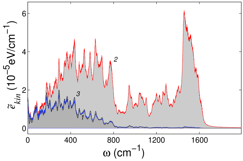
Figure 6: (Color online) Power spectral density of thermal vibrations of carbon nanotube C₃₀₀ atoms at temperature $T=300$K. Lines 1 (blue) and 2 (red) give the densities obtained within the semi-quantum and classical descriptions, respectively. Line 3 (black) shows the density obtained with the use if Eq. (37) for the system of quantum oscillators, where the discreteness of the spectrum was smoothed for convenience. The frequency spectrum of the mean kinetic energy per atom is shown.

Carbon nanotube is a rigid structure in which the anharmonicity of atomic dynamics at room temperature is weakly pronounced: as one can see from line 2 in Fig. 6, the characteristic Debye temperature of the carbon nanotube is very high, $T_{D}\sim\hbar\omega_{m}/k_{B}\approx 2400$K, where $\omega_{m}\approx 1640$ cm^-1 is the maximal phonon frequency in the system. Therefore we can obtain the temperature dependence of the carbon nanotube specific heat with the use of the spectrum of the harmonic (non-interacting) vibrational eigenmodes: $C(T)=dE(T)/dT$, where the average energy of the system $E(T)$ is given by Eq. (13). To obtain the eigenfrequencies $\Omega_{n}$, we have to find all the eigenvalues of the square symmetric matrix $\partial^{2}H/\partial{\rm\bf r}_{n}\partial{\rm\bf r}_{m}$ of the $3N\times 3N$ size: if $\lambda_{n}$ is one of the eigenvalues, the eigenfrequency is determined as $\Omega_{n}=\sqrt{\lambda_{n}/M_{n}}$. For $N=300$ atoms in the nanotube, we have $3N=900$ eigenmodes, from which the first 6 modes, which describe rigid translations and rotations of the nanotube, have zero frequency, $\Omega_{1}=\dots=\Omega_{6}=0$, while the other eigenfrequencies are nonzero and are distributed in the interval 25.1 cm${}^{-1}\leq\Omega_{n}\leq 1640.0$ cm^-1, $n=7,8,\dots,900$. We can obtain the temperature dependence of the nanotube specific heat with the use of Eq. (13):

$$C(T)=k_{B}\sum_{n=7}^{3N}\left(\frac{\hbar\Omega_{n}}{k_{B}T}\right)^{2}\frac{\exp(\hbar\Omega_{n}/k_{B}T)}{[\exp(\hbar\Omega_{n}/k_{B}T)-1]^{2}}$$ (35)

As one can see in Fig. 5, the nanotube specific heat in the quantum description monotonously goes to zero for $T\rightarrow 0$, and the effects of quantum statistics of phonons are essential for the carbon nanotube in the whole temperature range $T<500$K, in which the specific heat $C(T)$ of the nanotube is considerably less than the classical-statistics value $(3N-6)k_{B}$. This conclusion also applies to other carbon-based materials and systems with high Debye temperature like graphene, graphene nanoribbons, fullerene, diamond, diamond nanowires etc.

To model the nanotube stochastic dynamics in the semi-quantum approach, we will use the Langevin equations of motion (1) with random forces $\Xi_{n}=\{\xi_{\alpha n}\}_{\alpha=1}^{3}$ with the power spectral density, given by $\langle\xi_{\alpha n}\xi_{\beta m}\rangle_{\omega}=2M\Gamma k_{B}T\langle S_{1\alpha n}S_{1\beta m}\rangle_{\bar{\omega}}$, see Eq. (34). Here it is explicitly taken into account that zero-point oscillations do not contribute to the specific heat of the system, and therefore one needs to account only for the random functions, given by Eq. (32).

Therefore the semi-quantum approach in this case amounts to the integration of Eqs. (1) and (30), to find the average energy $\langle H\rangle=E(T)$ and the specific heat $C(T)=dE(T)/dT$ of the system. As one can see from Fig. 5, the temperature dependence of the carbon nanotube specific heat, obtained by studying the nanotube stochastic dynamics with color noise, coincides completely with the dependence, obtained from the spectrum of the harmonic vibrational eigenmodes in the system. Power spectral density of carbon atoms vibrations, see Fig. 6, shows that the semi-quantum approach describes the thermalization of only the low-frequency eigenmodes, with $\omega<\omega_{T}=k_{B}T/\hbar$. In such a way, the approach models the quantum freezing of the high-frequency eigenmodes at low temperature $T<T_{D}$. For the carbon nanotube, the classical description is definitely not valid at room temperature $T=300$K, when the characteristic frequency $\omega_{T}=208.5$ cm^-1 is much less than the maximal one in the system, $\omega_{m}=1640$ cm^-1, see Fig. 6.

It is worth mentioning in this connection that the obtained results for the temperature dependence of the specific heat of the carbon nanotube C₃₀₀ almost do not depend on the relaxation time $t_{r}$. All the five values of $t_{r}$, $t_{r}=0.1$, 0.2, 0.4, 0.8, 1.6 ps, give the same average energy $E(T)$ and specific heat $C(T)$ of the nanotube. One cannot use either too short $t_{r}$, when the system dynamics becomes the forced one, or too long $t_{r}$, which increases the computation time. We find that the optimal relaxation time for the carbon nanotube is $t_{r}=0.4$ ps.

Above we have introduced and discussed the lattice temperature of the system embedded in the Langevin thermostat with color noise determined by the quantum fluctuation-dissipation theorem, see Eqs. (14) and (17). But to compute the thermal conductivity, one also needs to determine the local temperature of the part of the molecular system, which is placed between two thermostats with different temperatures. In the classical-statistics approximation, the lattice temperature can be determined as the average double kinetic energy per mode (or per degree of freedom):

$$T=\frac{1}{3Nk_{B}}\langle\sum_{n=1}^{N}M\dot{\bf r}_{n}^{2}\rangle,$$ (36)

where $N$ is a number of atoms and is assumed that $3N-6\approx 3N$. As we have shown in Chapter III, such determination of temperature does not work in the semi-quantum approximation when one needs to deal with the density and population of vibrational (phonon) states. In this case the determination of temperature is given by Eq. (14) or by Eq. (17). But in the MD simulations, one can also use the determination of temperature, which is equivalent to the integral presentation of Eq. (12).

Having in mind further simulation of thermal conductivity, we omit in Eqs. (2) and (6) the zero-point contribution to the spectrum of the random forces. With the use of Eqs. (9), (12), (18) and (19), we find the average energy per mode (per degree of freedom) as

$$e(T)\equiv\frac{1}{3N}E(T)=\frac{1}{3N}\int_{0}^{\infty}\frac{\hbar\omega}{\exp(\hbar\omega/k_{B}T)-1}D(\omega)\frac{d\omega}{\pi}$$

$$=\frac{1}{3N}\sum_{n=7}^{3N}\frac{\hbar\Omega_{n}}{\exp(\hbar\Omega_{n}/k_{B}T)-1},$$ (37)

where $D(\omega)$ is density of vibrational states, cf. Eq. (11).

From the MD simulations, we can also measure the spectral density $\tilde{e}_{kin}(\omega)$ of the average double kinetic energy per mode $e_{kin}$ as

$$e_{kin}\equiv\frac{1}{3N}\sum_{n=1}^{N}\langle M_{n}\dot{\bf r}^{2}_{n}\rangle=\int_{0}^{\infty}\tilde{e}_{kin}(\omega)\frac{d\omega}{\pi}.$$ (38)

In the case of correct ”quantum”  level occupation, the both Eqs. (37) and (38) should correspond to the same value of temperature, therefore we obtain the following equation for the (numerical) determination of the lattice temperature:

$$e(T)=e_{kin}.$$ (39)

Since function $e(T)$ monotonously increases with $T$, Eq. (39) has a unique solution for the temperature. Similar equation, but with an account for zero-point oscillations, for the rescaling of MD temperature for an effective one was used in Ref. wang90 for quantum corrections of MD results. As we have mentioned above in discussion of Fig. 5, the neglect of zero-point oscillations in the computation of the average thermal energy leads to the feature that $e_{kin}\leq k_{B}T$ in general and $e_{kin}\ll k_{B}T$ for temperature much less than the Debye one, see also Fig. 11 (b) and (c) below.

Essentially one can use Eq. (39) for the determination of the lattice temperature only for the quantum-statistics population of $all$ phonon states. But the situation can emerge when high-frequency phonons have an excess excitation, in comparison with the Bose-Einstein distribution for the given temperature, see section VII below. In this case the lattice temperature $T$ can be determined with the use of only part of the phonon spectrum:

$$\frac{1}{3N}\int_{\omega_{1}}^{\omega_{2}}\frac{\hbar\omega}{\exp(\hbar\omega/k_{B}T)-1}D(\omega)\frac{d\omega}{\pi}=\int_{\omega_{1}}^{\omega_{2}}\tilde{e}_{kin}(\omega)\frac{d\omega}{\pi},$$ (40)

where $[\omega_{1},\omega_{2}]$ is the frequency interval with the Bose-Einstein distribution of the average energy per mode $\tilde{e}(\omega)$. For $\omega_{1}=0$, $\omega_{2}>\Omega_{max}+\Gamma$ and $k_{B}T\gg\hbar\omega_{2}$, Eq. (40) gives the classical definition of temperature, $e_{kin}=k_{B}T$. Clearly Eq. (39), which is more convenient for the numerical modeling, gives the correct value of lattice temperature only for $\omega_{1}=0$ and $\omega_{2}\geq\Omega_{max}+\Gamma$.

If the molecular system is completely embedded in the Langevin thermostat with color-noise random forces, their spectrum, given by Eq. (3), provides the correct ”quantum”  population of all the phonon states. As one can see in Fig. 6, at $T=300$K the spectral density of the average energy per mode $\tilde{e}_{kin}(\omega)$ in the $C_{300}$ carbon nanotube (red line 1) coincides exactly with the smoothed function $D(\omega)\hbar\omega/(\exp(\hbar\omega/k_{B}T)-1)/3N$ (black line 3). In this case Eq. (39) determines the temperature, which is exactly equal to the one of the thermostat.

VI Thermal conductivity of nanoribbon with rough edges

First we apply the semi-quantum approach for the molecular dynamics simulation of thermal conductivity in the nanoribbon with rough edges and harmonic interparticle potential. In such system the vibrational eigenmodes do not interact and the considered semi-quantum approach turns to be the exact one.

It was predicted analytically and confirmed by classical molecular dynamics simulations that rough edges of molecular nanoribbon (or nanowire) cause strong suppression of phonon thermal conductivity due to strong momentum-nonconserving phonon scattering kosevich1 ; kosevich2 . In the case of nonlinear interatomic potential, the ribbon has a finite, length-independent thermal conductivity, while in the case of harmonic interatomic potential, the thermal conductivity decreases with the ribbon length (and the ribbon behaves as a thermal insulator). Essentially for both interatomic potentials, the thermal conductivity increases with the length of the nanoribbon with perfect (atomically smooth) edges. In the case of harmonic interatomic potential, phonons in the nanoribbon with rough edges experience effective localization due to strong antiresonance multichannel reflection from side atomic oscillators in the rough edge layers (the Anderson-Fano-like localization due to interference effects in phonon backscattering), see kosevich1 ; kosevich2 . Apparently such strong backscattering can localize phonons with the wavelength shorter than the ribbon length. Within the classical description, such effect does not depend on temperature. But this picture will be changed if we take into account the quantum effects. The latter result in thermalization and correspondingly in participation in low temperature thermal transport of long wave phonons only. The long wave phonons are much less affected by surface roughness than the short wave phonons and therefore the effect of thermal conductivity suppression should decrease with the decrease of temperature. Below we demonstrate this effect within the proposed semi-quantum approach.

We consider the system which consists of $K$ parallel molecular chains in one plane kosevich2 . Let $k$ be the chain number, $n$ be the molecular number in the chain, then the equilibrium position of the $n$-th atom in the $k$-th chain will be $x_{k,n}^{0}=na+[1+(-1)^{k}]a/4$, $y_{k,n}^{0}=bk$, where $a$ and $b$ are, respectively, the intra- and interchain spatial periods, see Fig. 7.

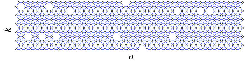
Figure 7: Molecular ribbon made of $K=12$ molecular chains. Density and widths of rough edges are $d=0.95$ and $K_{1}=4$, respectively. Lines connect the interacting atoms.

Only the longitudinal displacements are taken into account in a simplest scalar model of two-dimensional crystal: $x_{k,n}(t)=x_{k,n}^{0}+au_{k,n}(t)$, $y_{k,n}\equiv y_{k,n}^{0}$, where $u_{k,n}$ is a dimensionless longitudinal displacement of the $(k,n)$-th molecule from its equilibrium position. Hamiltonian of the system has the form as

$$H = \sum_{k=1}^{K}\sum_{n=1}^{N}\frac{1}{2}Ma^{2}\dot{u}_{kn}^{2}$$ (41)

$$+ E_{0}\sum_{k=1}^{K}\sum_{n=1}^{N-1}V(u_{k,n+1}-u_{k,n})+E_{0}\sum_{k=1}^{K}E_{k},$$

where $N$ is a number of molecules in each chain, $M$ is a mass of molecule, $E_{0}$ is a characteristic interaction energy, $V(\rho)$ is the dimensionless potential of the nearest-neighbor intrachain interactions, $\rho$ describes relative displacements of the nearest-neighbor atoms, $E_{k}$ describes the interchain interaction.

Dimensionless energy of the nearest-neighbor interchain interactions for odd $k$ is

$$E_{k}=\sum_{n=2}^{N}U(u_{k,n}-u_{k+1,n-1})+\sum_{n=1}^{N}U(u_{k+1,n}-u_{k,n}),$$ (42)

and for even $k$ is

$$E_{k}=\sum_{n=1}^{N}U(u_{k,n}-u_{k+1,n})+\sum_{n=1}^{N-1}U(u_{k+1,n+1}-u_{k,n}),$$ (43)

where $U(\rho)$ is the dimensionless potential of the nearest-neighbor interchain interaction.

We will consider a finite rectangular $(1\leq n\leq N,~{}1\leq k\leq K)$ with free edges, and harmonic intra- and interchain interaction potentials:

$$V(r)=r^{2}/2,~{}~{}U(r)=r^{2}/4.$$ (44)

For the convenience of the modeling, we introduce the dimensionless quantities: temperature $\tilde{T}=T/T_{0}$, time $\tilde{t}=t/t_{0}$, and energy $E=H/E_{0}$, where $T_{0}=\hbar^{2}/Ma^{2}k_{B}$, $t_{0}=\hbar/k_{B}T_{0}$, and $E_{0}=Ma^{2}/t_{0}^{2}$. Then the dimensionless Hamiltonian will have the form as

$${\cal H}=\sum_{k=1}^{K}\sum_{n=1}^{N}\frac{1}{2}\dot{u}_{m,n}^{2}+\sum_{k=1}^{K}\sum_{n=1}^{N-1}V(u_{k,n+1}-u_{k,n})+\sum_{k=1}^{K}E_{k},$$ (45)

where the dot denotes the derivative with respect to the dimensionless time $\tilde{t}$.

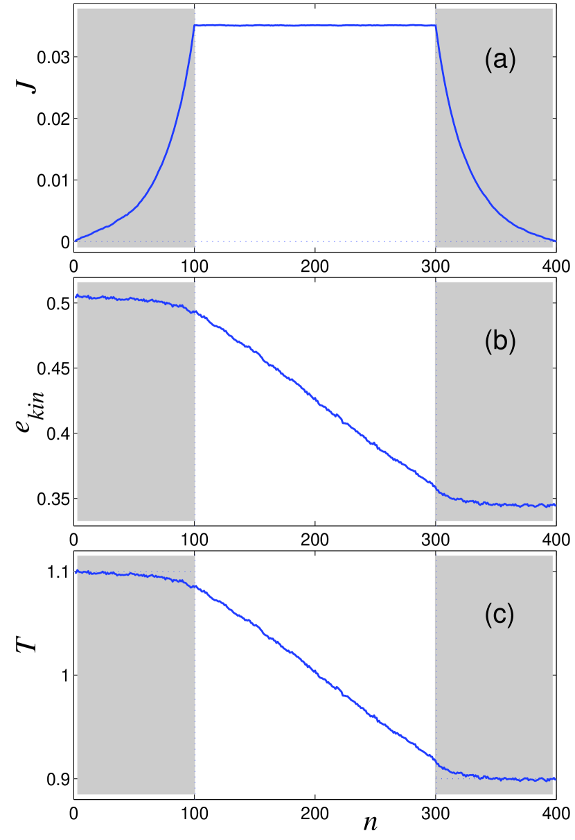
Figure 8: (Color online) Distribution of (a) local energy flux $J$, (b) local kinetic energy per mode $e_{kin}$ and (c) local temperature $T$ along the rough-edge ribbon (ribbon length $N=400$, width $K=12$, rough edges widths $K_{1}=4$, porosity of rough edges $p=0.05$). Gray arias indicate the ribbon ends, embedded in semi-quantum Langevin thermostats with temperatures $T_{\pm}=1\pm 0.1$.

For the dimensionless quantities, equations of motion will take the form:

$$\ddot{u}_{kn}=-\frac{\partial\cal H}{\partial u_{kn}}-\tilde{\Gamma}\dot{u}_{kn}+\eta_{kn},~{}~{}k=1,...,K,~{}n=1,...,N$$ (46)

where $\tilde{\Gamma}=\Gamma t_{0}$ is the dimensionless friction, and the dimensionless random forces $\eta_{kn}$ is the color noise with the correlation functions

$$\langle\eta_{kl}(s)\eta_{mn}(0)\rangle=2\tilde{\Gamma}\tilde{T}\delta_{km}\delta_{ln}\int_{-\infty}^{+\infty}p(\tilde{\omega},\tilde{T})\exp(-i\tilde{\omega}s)\frac{d\tilde{\omega}}{2\pi},$$ (47)

and dimensionless power spectral density

$$p(\tilde{\omega},\tilde{T})=\frac{1}{2}(\tilde{\omega}/\tilde{T})+\frac{\tilde{\omega}/\tilde{T}}{\exp(\tilde{\omega}/\tilde{T})-1},$$ (48)

where $\tilde{\omega}=\omega t_{0}$ is the dimensionless frequency. In the following we will deal only with the dimensionless quantities.

Phonons do not interact in the system with harmonic interparticle potential. Therefore the zero-point oscillations will not affect the thermal transport along the nanoribbon and can be not taken into the account. In the latter case we can consider the dimensionless random forces with the power spectra, given by $\langle\eta_{kn}\eta_{lm}\rangle_{\tilde{\omega}}=2\tilde{\Gamma}\tilde{T}\langle S_{1kn}S_{1lm}\rangle_{\bar{\omega}}$, cf. Eq. (34). Random forces in Eq. (46) are $\eta_{kn}(\tilde{t})=\eta_{kn}(\tau/\tilde{T})=\tilde{T}\sqrt{2\tilde{\Gamma}}S_{1kn}(\tau)$.

Within this approach, we will describe the temperature dependence of the nanoribbon thermal conductivity $\kappa(T)$. We embed the left end of the ribbon with length $N_{e}=100$ in the thermostat with temperature $T_{+}=1.1T$, while the right end embed in the thermostat with temperature $T_{-}=0.9T$. In this case the dynamics of the atoms with numbers $n=1,...,N_{e}$ is described by Langevin equations (46) with temperature $T=T_{+}$, the atoms with numbers $n=N-N_{e}+1,...,N$ are described by these equations with temperature $T=T_{-}$, while the atoms in the central part of the nanoribbon, with numbers $n=N_{e}+1,...,N-N_{e}$, are described by the frictionless equations, Eqs. (46) with $\tilde{\Gamma}=0$ and $\eta_{kn}\equiv 0$. We take the relaxation time $t_{r}=100$, at which the edge effects at the interfaces between the ribbon and the thermostats are not essential. We integrate the equations of motion to find the stationary energy flux $J$ along the ribbon.

To determine the temperature profile, first we find energy per mode at the longitudinal coordinate $x=na$ by averaging the distribution across the ribbon of the scalar-model double kinetic energy:

$$e_{kin}(n)=\frac{1}{K}\sum_{j=1}^{K}\langle\dot{u}^{2}_{n,j}\rangle.$$ (49)

Since in the ribbon with a constant average width the phonon spectrum does not depend on the longitudinal coordinate and the inter-mode interaction is absent in the harmonic system, we can determine the local temperature from the equation $e_{kin}(n)=e(T_{n})$, similar to Eq. (39). Figure 8 shows the distribution along the ribbon of energy flux $J$, kinetic energy per mode $e_{kin}$ and temperature $T$. There is a stationary flux in the area between the thermostats. Since the temperature distribution of phonon frequencies in the ribbon with harmonic interactions is determined by the Langevin thermostats with Bose-Einstein color noise, we can uniquely determine the local temperature $T_{n}$, which monotonously changes from the value $T_{+}$ at the left end to the value $T_{-}$ at the right end with a linear gradient, see Fig. 8(c).

Then the dimensionless thermal conductivity of the finite-length ribbon can be found as

$$\kappa(N,T)=(N-2N_{e})J/[K(T_{+}-T_{-})].$$ (50)

In the ribbon with perfect (atomically smooth) edges, phonons have infinite mean free path and therefore the energy flux $J$ does not depend on the length of the central part of the ribbon $N_{c}=N-2N_{e}$. In this case, as one can conclude from Eq. (50), the thermal conductivity increases linearly with $N_{c}$ and therefore such ribbon behaves as an ideal (ballistic) thermal conductor. In the absence of anharmonicity of interatomic interactions, this conclusion is valid for any temperature.

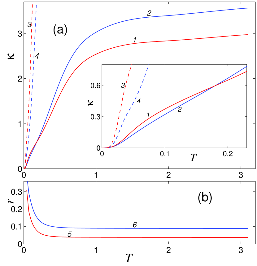
Figure 9: (Color online) (a) Thermal conductivity $\kappa$ of rough-edge ribbon (ribbon width $K=12$, rough edges widths $K_{1}=4$, porosity of rough edges $p=0.05$) versus temperature $T$ for ribbon length $N=600$ (line 1) and $N=400$ (line 2). Dashed lines 3 and 4 give the dependencies for perfect nanoribbons (with zero porosity of edges, $p=0$) with $N=600$ and $N=400$, respectively. Inset shows the low-temperature limit, $T\leq 0.22$. (b) Factor of thermal conductivity suppression by rough edges $r$ versus temperature for ribbon length $N=600$ (line 5) and $N=400$ (line 6).

We consider a ribbon which consists of $K=12$ molecular chains. To model the roughness of the ribbon edges, we delete with probability $p=1-d$ some atoms from the chains with numbers $k=1,...,K_{1}$ and $k=K-K_{1}+1,...,K$. Here $K_{1}$ is a width of the rough edges, $0\leq d\leq 1$ is their atomic density and the parameter $p$ determines in fact the porosity of the ribbon lattice in the defect edges. We take in the following $K_{1}=4$ and $p=0.05$. We computed the thermal conductivity $\kappa(N,T)$ for $N=400$ ($N_{c}=200$) and $N=600$ ($N_{c}=400$), see Fig. 9. As one can see from this figure, at high (dimensionless) temperature the ribbon with the length $N=600$ has lower thermal conductivity than the ribbon with length $N=400$. This means that the ribbon behaves much like thermal insulator, in which the thermal conductivity decreases with the length of the system, see also kosevich2 . But the situation is changed for low temperature, for $T<0.18$, when the longer ribbon has the higher thermal conductivity, as in the case of perfect nanoribbons, see the inset in Fig. 9 (a).

In this connection we can define the factor of thermal conductivity suppression by rough edges $r(T,N)=\kappa_{1}(N,T)/\kappa_{0}(N,T)$, where $\kappa_{0}(N,T)$ is thermal conductivity of a ribbon with ideal (atomically smooth) edges and length $N$, $\kappa_{1}(N,T)$ is thermal conductivity of the rough-edge ribbon with the same length and width. As one can see from Fig. 8 (b), the rough edges suppress the thermal conductivity for all temperatures, $r<1$ for $T>0$, but the suppression monotonously decreases with the decrease of temperature: for $T\rightarrow 0$ the thermal conductivities of the ideal- and rough-edge ribbons flatten, $r\rightarrow 1$. This means that long wave acoustic phonons are not scattered by surface roughness and therefore at low enough temperature the rough-edge quantum ribbon becomes an ideal (ballistic) thermal conductor, in which the thermal conductivity increases with the conductor length. This in turn means that at low enough temperature we approach the limit of ballistic quantum thermal transport, when the value of thermal conductance $G_{th}=J/\Delta T$, the ratio of the thermal flux $J$ through the quasi-one-dimensional thermal conductor to the temperature difference $\Delta T=T_{+}-T_{-}$, has a quantized value $\pi^{2}k_{B}^{2}T/3h$ (per each of the four massless acoustic modes of the quasi-one-dimensional waveguide), which does not depend on the material properties (and perfectness) of the thermal conductor, see, e.g., Refs. maynard ; rego ; schwab . This property of low-temperature thermal transport is in drastic contrast to that in the classical high-temperature regime, in which the same quasi-one-dimensional rough-edge nanoribbon behaves as a thermal insulator, in which the thermal conductivity decreases with the insulator length, see Ref. kosevich2 .

VII Modeling of heat transport in carbon nanotube

The computation of the thermal conductivity can be performed by two methods. In the first method, the system is thermalized with the use of equilibrium molecular dynamics and then the interaction with the thermostat is switched off. The current-current correlation function in the system is computed and the coefficient of thermal conductivity is found with the help of Green-Kubo formula based on this correlation function. In the second method, the method of non-equilibrium dynamics, the direct modeling of thermal transport is performed. For this purpose, two ends of the quasi-one-dimensional system are embedded in two thermostats with different temperatures. The stationary flux of energy is computed and the coefficient of thermal conductivity is determined from the known energy flux, temperature difference and length of the system. In the approach based on the non-equilibrium dynamics, the correct use of thermostats is important. The Langevin thermostat can be used in such approach.

The both methods model the heat transport within the classical Newtonian dynamics and therefore do not allow to take into account the quantum effects. These methods can be justified only for high enough temperature when the statistics of the system becomes completely classical. Nevertheless the method of the non-equilibrium dynamics can be easily adapted for the use in the semi-quantum approach to molecular dynamics modeling of thermal transport. Below we demonstrate this by example of a carbon nanotube.

For the classical modeling of heat transport, we consider finite nanotube with chirality index (5,5) (see Fig. 4), and embed its left end in Langevin thermostat with temperature $T_{+}=1.1T$ and the right end in a thermostat with temperature $T_{-}=0.9T$, where $T$ is a temperature at which the thermal conductivity will be determined. For this purpose the dynamics of the atoms at the left (right) end of the nanotube should be described by the Langevin equations (1) with a white noise with the correlation function given by Eq. (5) with temperature $T=T_{+}$ ($T_{-}$). Dynamics of the atoms in the central part of the nanotube we describe with the Hamilton equations

$$M_{n}\ddot{\rm\bf r}_{n}=-\partial H/\partial{\rm\bf r}_{n}.$$ (51)

This allows us to find the distribution of temperature $T(x)$ and energy flux $J(x)$ along the nanotube, see Fig. 10. The detailed calculation of these quantities can be found in Ref. savin1 . In the classical molecular dynamics description, temperature of a particle can be determined through its average double kinetic energy per mode (or per degree of freedom) as

$$T=M\langle\dot{x}^{2}+\dot{y}^{2}+\dot{z}^{2}\rangle/3k_{B}\equiv e_{kin}/k_{B},$$ (52)

where $M$ and $(x,y,z)$ are particle mass and cartesian coordinates.

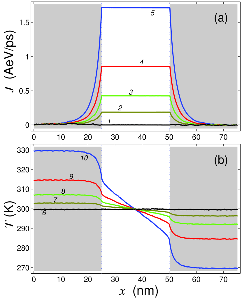
Figure 10: (Color online) Distribution of (a) local energy flux $J$ and (b) local temperature $T$ along the carbon nanotube (5,5) C₆₀₂₀, $x$ axis is along the nanotube axis. Nanotube length is $L=75.04$ nm. Gray arias indicate the nanotube ends, embedded in classical Langevin thermostats with temperatures $T_{\pm}=(1\pm\delta)300$K, for $\delta=0$; 0.0125; 0.025; 0.05; 0.1 (curves 1 and 6; 2 and 7; 3 and 8; 4 and 9; 5 and 10, respectively).

To illustrate the modeling of heat transport, we consider a nanotube with a fixed length $L=75.04$ nm (which corresponds to N=6020 atoms) and embed its ends with lengths $L_{e}=L/3$ in classical Langevin thermostats with temperature $T_{\pm}=(1\pm\delta)300$ K, where $\delta=0$, 0.0125, 0.025, 0.05, 0.1. For the relaxation time, we take $t_{r}=0.4$ ps. As one can see in Fig. 10, for $\delta=0$ when the ends have the same temperature $T_{+}=T_{-}=300$ K, the temperature is a constant along the whole nanotube ($T(x)\equiv 300$ K) and there is no heat flux in the circuit ($J(x)\equiv 0$). For $T_{+}>T_{-}$ ($\delta>0$), the linear temperature gradient $T(x)$ and heat flux are formed in the central part of the nanotube: $J(x)\equiv J>0$ for $L_{e}\leq x\leq L-L_{e}$. This allows to determine the thermal conductivity of the nanotube of length $L$ as

$$\kappa(L,T)=(L-2L_{e})J/S(T_{+}-T_{-}),$$ (53)

where $S=\pi r^{2}$ is nanotube cross section [radius $r$ is equal to 0.335 nm for the (5,5) single-walled nanotube]. One can obtain more accurate estimate for the thermal conductivity from the temperature profile in the central part of the nanotube:

$$\bar{\kappa}=(L-2L_{e})J/S[T(L_{e})-T(L-L_{e})],$$ (54)

where $T(x)$ is a distribution of the particle kinetic energy (temperature) along the nanotube. The definition of thermal conductivity, given by Eq. (54), allows one to separate boundary resistances from the thermal resistance of the nanotube by itself. The boundary (Kapitza) resistance causes finite difference between the temperatures in the bulk of the heat reservoir and just at the interface with the nanotube, see Fig. 10(b). Since one has $T(L_{e})<T_{+}$ and $T(L-L_{e})>T_{-}$ at the interfaces between the ends embedded in the thermostats and the central part of the nanotube, Eqs. (54) always give higher values of thermal conductivity than Eq. (53) does: $\bar{\kappa}>\kappa$. Dependencies of the obtained values of $\kappa$ and $\bar{\kappa}$ on the temperature difference at the ends of the nanotube, $\Delta T=2\delta\times 300$ K, are presented in Table 2.

Table 2: Heat flux $J$, thermal conductivities $\kappa$ and $\bar{\kappa}$ of the (5,5) carbon nanotube of length $L=75.04$ nm versus temperature difference at the ends $\Delta T=T_{+}-T_{-}$ [mean temperature is $T=(T_{+}+T_{-})/2=300$ K, lengths of the embedded in thermostats ends are $L_{e}=L/3$, relaxation time is $t_{r}=0.4$ ps]. The values were obtained with the use of classical molecular dynamics (CMD) and of semi-quantum molecular dynamics (SQMD). The values of $\kappa$ and $\bar{\kappa}$ have been calculated with the use of Eqs. (53) and (54).

	CMD		SQMD
$\Delta T$ (K)	$J$ (eVÅ/ps)	$\kappa$ $(\bar{\kappa})$ (W/mK)	$J$ (eVÅ/ps)	$\kappa$ $(\bar{\kappa})$ (W/mK)
60.0	1.714	260.0 (448)	0.659	99.9 (260)
30.0	0.856	259.5 (447)	0.315	95.4 (249)
15.0	0.426	258.6 (443)	0.154	93.4 (244)
7.5	0.210	257.1 (436)	0.077	93.0 (243)

As one can see in Table 2, for $\Delta T\leq 60$ K the halving of the temperature difference results in the halving of the energy flux $J$. Since in this case the flux is proportional to the temperature difference, the determination of the thermal conductivity $\kappa$ ($\bar{\kappa}$) does not depend on the value of $\Delta T$. It is worth mentioning that the accuracy of the determination of the energy flux $J$ decreases with the decrease of $\Delta T$. Therefore the most convenient for the MD modeling of thermal conductivity are the values of the temperatures at the nanotube ends as $T_{+}=1.1T$ and $T_{-}=0.9T$, although a relatively high gradient of temperature is formed in this case (0.8 K/nm for $T=300$ K).

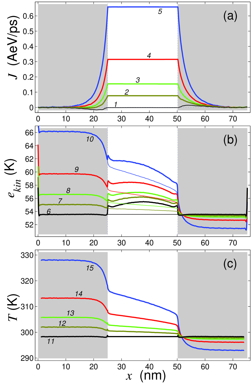
Figure 11: (Color online) Distribution of (a) local energy flux $J(x)$, (b) local kinetic energy per mode $e_{kin}(x)$, and (c) local temperature $T(x)$ along the carbon nanotube (5,5) C₆₀₂₀ axis $x$. Nanotube length is $L=75.04$ nm. Gray arias indicate the nanotube ends, embedded in semi-quantum Langevin thermostats with temperatures $T_{\pm}=(1\pm\delta)300$K, for $\delta=0$; 0.0125; 0.025; 0.05; 0.1, curves 1 and 6; 2 and 7; 3 and 8; 4 and 9; 5 and 10, respectively. Thin lines show distributions of average particle energies $\bar{e}_{kin}(x)$ in the central part of the nanotube without the artefact surplus thermal energy $\Delta e_{kin}(x)$. Local temperature $T(x)$ in (c) is determined from Eq. (39) with the use of $\bar{e}_{kin}(x)$, given by thin lines in (b).

For the semi-quantum MD modeling of heat transport, we must use the Langevin equations (1) with the random forces $\xi_{\alpha n}$ with the power spectral density, given by $\langle\xi_{\alpha n}\xi_{\beta m}\rangle_{\omega}=2M\Gamma k_{B}T\langle S_{1\alpha n}S_{1\beta m}\rangle_{\bar{\omega}}$, see Eq. (34), with temperature $T=T_{+}$ or $T=T_{-}$. The color noise is determined as $\xi_{\alpha n}(t)=\xi_{\alpha n}(\hbar\tau/k_{B}T_{\pm})=k_{B}T_{\pm}\sqrt{2M\Gamma/\hbar}S_{1\alpha n}(\tau)$. The zero-point oscillations do not contribute to the thermal transport, and therefore they will not be taken into account in the following and in all the formulas below we will put $S_{0\alpha n}(\tau)\equiv 0$. The thermal conductivity $\kappa$ can be found with the use of Eq. (53).

In the semi-quantum MD modeling, the mean value of particle kinetic energy $e_{kin}$ does not coincide with the temperature. This value depends not only on the temperature, but also on the density of phonon states. For example, the carbon atoms at the end hemispheres of the nanotube have different vibrational spectrum than the atoms in the central part of the nanotube. As one can see in Fig. 11 (b), at the very ends of the nanotube, for $x$ close to 0 and to 75 nm, the mean kinetic energy of carbon atoms is higher than that in the central part of the nanotube. In the central part of the nanotube, all the atoms have the same vibrational spectrum. Here $e_{kin}$ depends unambiguously on temperature and therefore the distribution of kinetic energy along the nanotube characterizes unambiguously the distribution of temperature.

Carbon nanotube is a stiff molecular system with weakly nonlinear dynamics. One can compute its vibrational spectrum and then use Eq. (39) to determine the local temperature in the system.

We consider the nanotube of length $L=75.04$ nm, which ends with the length $L_{e}=L/3$ are embedded into semi-quantum Langevin thermostats with temperatures $T_{\pm}=(1\pm\delta)300$ K (when $\delta=0$, 0.0125, 0.025, 0.05, 0.1). As one can see in Fig. 11 (b), for $T_{+}=T_{-}=300$ K ($\delta=0$) the mean particle kinetic energy $e_{kin}$ is not constant along the nanotube. In the central part, which does not interact directly with the thermostats, particles have higher thermal energy than in the end parts, which do interact directly with the thermostats. For the end parts the mean kinetic energy is $e_{kin}(T_{\pm})=53.5$ K, while in the central part one has $e_{kin}(T_{\pm})\leq e_{kin}(x)<55.5$ K. The surplus kinetic energy $\Delta e_{kin}(x)=e_{kin}(x)-e_{kin}(T_{\pm})$, which is $0\leq\Delta e_{kin}(x)<2K$, is an artefact of the semi-quantum molecular dynamics approach when the latter is applied to nonlinear lattice, but it does not produce any thermal flux: $J(x)=0$ for $L_{e}<x<L-L_{e}$, see Fig. 11 (a).

The appearance of the surplus kinetic energy in the nonlinear system is related with phonon interaction caused by the anharmonicity, which induces the transfer of energy from the low-frequency modes to the high-frequency ones. In the nanotube ends, such transfer is suppressed by viscous friction, but in the central part of the nanotube it can result in the surplus excitation of the high-frequency modes. In the case of the white-noise heat baths, such inter-mode transfer does not occur because of the equipartition excitation. The inter-mode transfer results in surplus excitation of high-frequency modes in the central part of the nanotube, which ends are embedded in color-noise thermostats. The analysis of the vibrational spectrum shows that weakly anharmonic interparticle potential in the carbon nanotube results in a slight accumulation of energy in the high-frequency modes, with $\omega>900$ cm^-1, while the low-frequency modes, with $\omega<900$ cm^-1, follow the Bose-Einstein distribution, see Fig. 12. As it was explained above in connection with the quantum definition of the lattice temperature, see Eqs. (14) and (17), this means that the high-frequency modes possess higher effective temperature (and therefore are ”hot phonons”) then the lattice temperature, which is determined in turn by the Bose-Einstein distribution of the low-frequency modes.

For the system with the harmonic interparticle potential, the Bose-Einstein distribution is valid for all phonon modes in all the lattice system with the ends, embedded in color-noise thermostats. Indeed, as we have shown in Section V, there is no surplus excitation of high-frequency modes in the central part of the nanoribbon with the $harmonic$ interparticle potential.

For $T_{+}>T_{-}$ ($\delta>0$), a constant heat flux is formed in the central part of the nanotube ($J(x)\equiv J>0$ for $L_{e}<x<L-L_{e}$), which is proportional to the temperature difference $\Delta T=T_{+}-T_{-}$, see Table 2. As one can see in Fig. 11 (b), the distribution of local kinetic energy per mode $e_{kin}(x)$ has a nonlinear form for $L_{e}<x<L-L_{e}$. But after the subtraction of the artefact surplus contribution $\Delta e_{kin}(x)$ from the average kinetic energy $e_{kin}(x)$, the remaining local energy $\bar{e}_{kin}(x)$ has a linear slope. If one determines the local temperature $T(x)$ from the distribution of the local energy $\bar{e}_{kin}(x)$ with the use of Eq. (39), one gets the linear distribution of local temperature along the tube, see Fig. 11 (c). The same linear distribution of local temperature can also be obtained from Eq. (40), in which the integration over frequencies is performed in the low-frequency domain $\omega_{1}=0\leq\omega<\omega_{2}=900$ cm^-1. As one can see in Fig.  12, in this frequency domain the vibrational spectrum has a correct Bose-Einstein distribution, which allows the correct definition of temperature with the use of Eq. (39) in all parts, embedded ends and free central part, of the nanosystem. The linear distribution of local temperature along the tube allows in turn to determine more accurately the thermal conductivity of the system with the use of Eq. (54).

As one can see from Table 2, for $\Delta T<60$ K the value of thermal conductivity changes only weakly with the change of temperature difference. Thus for the numerical modeling, one can use $T_{\pm}=(1\pm\delta)T$ with $\delta=0.1$. Such temperature difference allows one to find rather fast the distribution of the heat flux and temperature along the nanotube, and the obtained value of the thermal conductivity $\kappa$ differs little from the values obtained for smaller $\delta$.

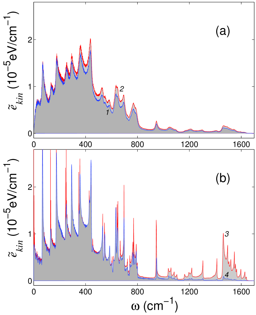
Figure 12: (Color online) Power spectral density of thermal vibrations in carbon nanotube (5,5) with length $L=75.04$ nm (a) for the atoms at the left end with temperature $T_{+}=330$ K (curve 2, red), right end with temperature $T_{-}=270$ K (curve 1, blue). (b) Line 3 (red) gives vibrational spectral density in the central part of the nanotube, which does not interact with the thermostats, line 4 (blue) gives the spectral density given by Eq. (37) for the corresponding system of quantum oscillators. The frequency spectrum of the mean kinetic energy per atom is shown.

Now we turn to the analysis of the vibrational frequency spectrum of carbon atoms near the nanotube ends embedded in thermostats with different temperatures, $T_{+}=330$ K and $T_{-}=270$ K, and in the nanotube central part. As one can see in Fig. 12, the power spectral density of thermal vibrations at the nanotube ends corresponds to the quantum statistics of phonons. But there are some distinctions in the nanotube central part, namely the high-frequency modes with frequencies $\omega>900$ cm^-1 are excited more strongly. This effect is related with the phonon interaction caused by anharmonicity, which induces the transfer of energy from the low-frequency vibrations to the high-frequency ones. In the nanotube ends, such transfer is suppressed by viscous friction, but in the central part of the nanotube it can result in the surplus (artefact) excitation of the high-frequency modes. As one can see from Fig. 12 (b), this effect is rather weak. It does not change the heat flux considerably for the used values of the nanotube length. It is worth mentioning in this connection that the high-frequency modes, which are revealed in Fig. 12 (b) for $\omega>900$ cm^-1, determine, via Eq. (14) or Eq. (17), the effective temperature of hot phonons, which is higher than the temperature of the equilibrium, Bose-Einstein, phonons. But the surplus hot-phonon temperature, similar to the surplus kinetic energy of the particles in the central part of the nanotube, shown in Fig. 11 (b), does not contribute to the linear distribution of the temperature and therefore to the thermal conductivity of the nanotube.

The difference in the power spectral density close to zero frequency in the end, Fig. 12 (a), and central, Fig. 12 (b), parts of the nanotube is related with the use of the effective fix-end and free-end boundary conditions in the simulation of corresponding spectra.

We would like to mention that the obtained results for the temperature dependence of the specific heat and thermal flux in the considered carbon nanotubes almost do not depend on the considered relaxation times $t_{r}=0.1$, 0.2, 0.4, 0.8 ps. The longer relaxation time increases the computation time. The steady-state heat transport established longer time and the computation of the mean values requires the integration along longer phase-space trajectories. The shorter relaxation time the effective viscosity smears out vibrational spectra of particles interacting with the thermostats. It can also increase the reflectivity of high-frequency phonons at the interfaces between the nanotube central part and the thermostats. The optimal relaxation time for the carbon nanotube is $t_{r}=0.4$ ps.

Now we consider the nanotube of the fixed length $L=50.08$ nm (which corresponds to $N=4020$ atoms), with $L_{e}=L/4$ and $t_{r}=0.4$ ps. Temperature dependence of the thermal conductivity of such nanotube is shown in Fig. 13. As one can see from this figure, within the classical description the thermal conductivity $\kappa_{1}$ monotonously increases with the decrease of temperature. This property of ”classical”  thermal conductivity is related with the decrease of anharmonicity of lattice dynamics with the decrease of temperature, which in turn results in the increase of phonon mean free path. But the situation changes drastically with an account for quantum statistics of phonons. In the semi-quantum description, thermal conductivity $\kappa_{2}$ first increases with the decrease of temperature from the high enough one but then it reaches its maximal value at $T=350$K and monotonously decreases to zero ($\kappa_{2}\rightarrow 0$ for $T\rightarrow 0$). Such temperature dependence of thermal conductivity, which is characteristic for solids peierls ; ziman , is related with the quantum decrease of the specific heat of the system. This is confirmed by the property that at low temperature $T\leq 250$K the thermal conductivity of the nanotube in the semi-quantum approach $\kappa_{2}(T)$ is described with high accuracy by the relation $\kappa_{2}(T)\approx c(T)\kappa_{1}(T)$, where $\kappa_{1}(T)$ is thermal conductivity of the carbon nanotube computed within the classical description, $c(T)=C(T)/3Nk_{B}$ is nanotube dimensionless specific heat at temperature $T$, see Figs. 5 and 13.

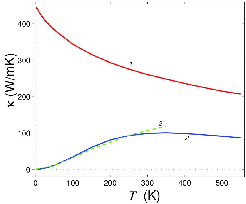
Figure 13: (Color online) Temperature dependence of thermal conductivity $\kappa_{i}$, $(i=1,2)$, of the carbon nanotube (5,5) with length $L=50.08$ nm: solid lines 1 and 2 are obtained within the classical and semi-quantum descriptions, respectively; dashed line 3 gives the temperature dependence $c(T)\kappa_{1}(T)$, where $c(T)=C(T)/3Nk_{B}$ is dimensionless specific heat of the carbon nanotube at temperature $T$.

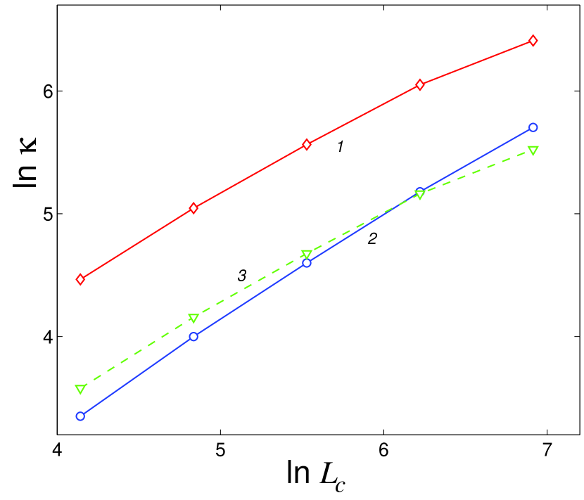
Figure 14: (Color online) Thermal conductivity $\kappa$ versus length of the central part $L_{c}=L-2L_{e}$ of the carbon nanotube (5,5) obtained with the use of classical (solid line 1) and semi-quantum (solid line 2) descriptions, and thermal conductivity $c(T)\kappa_{1}(T)$ (dashed line 3, as line 3 in Fig. 11) at $T=300$K. The length $L_{c}$ is measured in Å, the thermal conductivity $\kappa$ - in W/mK.

Length dependence of the nanotube thermal conductivity is shown in Fig. 14. As one can see from this figure, both methods give monotonous increase of the thermal conductivity with the nanotube length. The semi-quantum description gives the lower value of the conductivity than the classical one for all the considered nanotube lengths. As one can see from this figure, line 2 lies below line 3 for relatively short nanotubes, which is consistent with Fig. 13. But at some nanotube length the line 2 intersects the line 3. This means that for longer nanotube lengths the mean free path of ”semi-quantum” phonons is larger than that of purely ”classical” phonons. This in turn is related with the decrease in general of phonon mean free path with phonon frequency and the property that the mean frequency of semi-quantum phonons is always lower than that of classical phonons. The intersection at some nanotube length of the line 2 with line 3 in Figs.  13 and 14 means that short enough nanotubes effectively filter out the high-frequency and short-mean-free-path phonons, as it occurs in mesoscopic one-dimensional samples, see, e.g., Ref. maynard . Line 2 should intersect the line 1 at even longer lengths, when thermal conductivity of the ”semi-quantum” nanotube will become larger than that of purely ”classical” nanotube. Figure 15 (b) below shows that similar situation can also be realized in a nanoribbon. Concerning carbon nanotubes, at $T=300$K such intersection can be realized only in very long nanotubes because of their very high Debye temperature (which in fact exceeds the melting temperature of the material).

VIII Thermal conductivity of nanoribbon with periodic interatomic potentials

In order to demonstrate the characteristic temperature dependence of thermal conductivity of quantum low-dimensional system with strongly nonlinear interatomic interactions, we consider a nanoribbon with periodic interatomic potentials and perfect (atomically smooth) edges, cf. Eqs. (41)–(44):

$$V(r)=\epsilon_{1}[1-\cos(r)],~{}~{}~{}U(r)=\epsilon_{2}[1-\cos(r)]~{}.$$ (55)

In the following we will consider $\epsilon_{1}=1$, $\epsilon_{2}=0.5$, when for small relative displacements of the nearest-neighbor atoms $r$ the potentials (55) will coincide with the harmonic potentials given by Eq. (44). With the periodic interatomic potentials, given by Eq. (55), the ribbon becomes a system of coupled rotators.

A chain of coupled rotators presents a unique translationally-invariant one-dimensional system with a finite thermal conductivity giardina ; savin2 . In such system rotobreathers can be excited, which cause strong momentum-nonconserving scattering of phonons and result in finite thermal conductivity of the translational-invariant system. The density of rotobreathers increases with temperature increase and correspondingly the phonon mean free path decreases. In the classical description, this causes the monotonous decrease of thermal conductivity $\kappa$ with the increase of temperature: $\kappa\rightarrow 0$ for $T\rightarrow\infty$. In the opposite limit $T\rightarrow 0$, the phonon mean free path monotonously increases and therefore the thermal conductivity diverges: $\kappa\rightarrow\infty$ for $T\rightarrow 0$.

We consider a ribbon with a width $K=2$ and length $N=800$. We embed the ribbon ends with length $N_{e}=300$ each into Langevin thermostats with the color noise with temperature $T_{+}=1.1T$ and $T_{-}=0.9T$ in the left and right edge, respectively. For the relaxation time, we take $t_{r}=100$. Integration of Eqs. (46) for $n=1,...,N_{e}$ and $n=N-N_{e}+1,...,N$, and of frictionless equations, Eqs. (46) with $\tilde{\Gamma}=0$ and $\eta_{kn}$, for $n=N_{e}+1,...,N-N_{e}$, allows us to find an average energy flux along the ribbon $J$. With the use of Eq. (50), we then obtain the thermal conductivity of the finite-length nanoribbon.

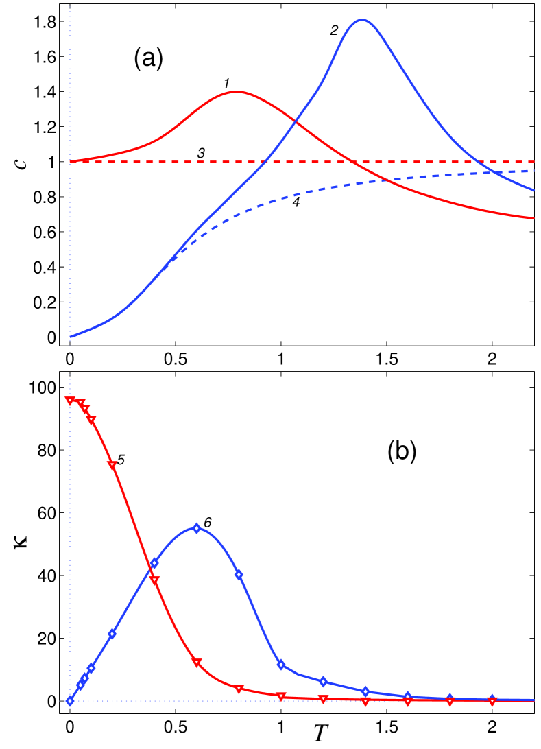
Figure 15: (Color online) (a) Specific heat $c$ of an ideal-edge ribbon with periodic interatomic potential (55) versus temperature $T$, obtained within the classical (line 1) and semi-quantum (line 2) descriptions. Dashed lines 3 and 4 show the dependencies for the nanoribbon with the harmonic interatomic potential (44) within, respectively, the classical and semi-quantum descriptions. (b) Thermal conductivity $\kappa$ versus temperature $T$ for the ribbon with length $N=800$ and width $K=2$ (the length of each of the two ends embedded into the thermostats with different temperatures is $N_{e}=300$): lines 5 and 6 give the results obtained within the classical and semi-quantum descriptions, respectively.

Results of numerical modeling are presented in Fig. 15. As one can see from the temperature dependence of the nanoribbon specific heat, Fig. 15 (a), within the semi-quantum description the anharmonicity of atomic dynamics starts to show up for $T>0.5$. Just at this temperature specific heat of the ribbon with the nonlinear interatomic potentials (55) starts to deviate from the specific heat of the ribbon with harmonic potentials (44), see Fig. 15 (a), line 2. It is worth mentioning that in the classical description the anharmonicity of lattice dynamics starts to show up for lower temperatures than that in the semi-quantum approach. This is related with the property that the anharmonicity is more pronounced in the dynamics of short wave phonons and therefore the quantum freezing out of the high frequency oscillations results in the effective decreasing of the dynamics anharmonicity (nonlinearity) at low temperature.

In the classical description, the thermal conductivity of the ribbon with nonlinear interatomic potentials (55) decreases monotonously with the increase in temperature: $\kappa\rightarrow 0$ for $T\rightarrow\infty$, see Fig. 15 (b), line 5. Within the semi-quantum description, the ribbon thermal conductivity reaches its maximal value at $T=0.6$. For the lower and higher temperatures, the thermal conductivity decreases, $\kappa\rightarrow 0$ for $T\rightarrow 0$ and $\kappa\rightarrow 0$ for $T\rightarrow\infty$, see Fig. 15 (b), line 6. For the low temperature $T<0.5$, system dynamics becomes almost linear when phonons propagate along the ribbon almost ballistically and the decrease of thermal conductivity is related with the quantum decrease of the specific heat. In this low temperature limit the thermal conductance of a short enough ribbon, in which phonon mean free path is longer than the ribbon length, can reach the lowest (quantum) value which has a linear temperature dependence, see line 6 in Fig. 15 (b) and compare the corresponding limit for the rough-edge ribbons, shown in Fig. 9, (a) and (b).

For temperature $T>0.4$, the semi-quantum description gives higher value for the thermal conductivity than that of the classical description. This is also related with the quantum freezing out of the high-frequency oscillations, which results in the decrease of the mean frequency of thermal phonons and correspondingly in the increase of phonon mean free path and phonon thermal conductivity. Therefore for $T>0.4$ the effect of the increase of phonon mean free path exceeds the effect of the decrease of low temperature specific heat. At high temperature, when phonons can be described with the classical statistics, the thermal conductivities given by the classical and semi-quantum descriptions merge, but the conductivity given by the semi-quantum description is always higher because of higher phonon mean free path under the equal, classical and semi-quantum, specific heats. The temperature dependence of thermal conductivity, given by line 6 in Fig. 15 (b), reminds the known temperature dependence of thermal conductivity in insulators, when the temperature of maximal thermal conductivity separates the low-temperature boundary-scattering regime from the high-temperature anharmonic Umklapp-scattering regime, see, e.g., Refs. peierls ; ziman ; klitsner ; han . In the case of the nanoribbon with periodic interatomic potentials and perfect edges, the maximal thermal conductivity, clearly displayed by curve 6 in Fig. 15 (b), is reached for the temperature, at which phonon mean free pass, which is determined in this system by the anharmonic scattering, levels off with the ribbon length. For the higher temperature, the phonon mean free pass becomes shorter then the ribbon length. Figure 15 (b) presents one of the main results of this work.

IX Summary

In summary, we present a detailed description of semi-quantum molecular dynamics approach in which the dynamics of the system is described with the use of classical Newtonian equations of motion while the effects of phonon quantum statistics are introduced through random Langevin-like forces with a specific power spectral density (the color noise). We describe the determination of temperature in quantum lattice systems, to which the equipartition limit is not applied. We show that one can determine the temperature of such system from the measured power spectrum and temperature- and relaxation-rate-independent density of vibrational (phonon) states. We have applied the semi-quantum molecular dynamics approach to the modeling of thermal properties and heat transport in different low-dimensional nanostructures. We have simulated specific heat and heat transport in carbon nanotubes, as well as the heat transport in molecular nanoribbons with perfect (atomically smooth) and rough (porous) edges, and in nanoribbons with strongly anharmonic periodic interatomic potentials. We have shown that the effects of quantum statistics of phonons are essential for the carbon nanotube in the whole temperature range $T<500$K, in which the values of the specific heat and thermal conductivity of the nanotube are considerably less than that obtained within the description based on classical statistics of phonons. This conclusion is also applicable to other carbon-based materials and systems with high Debye temperature like graphene, graphene nanoribbons, fullerene, diamond, diamond nanowires etc. We have shown that quantum statistics of phonons and porosity of edge layers dramatically change low temperature thermal conductivity of molecular nanoribbons in comparison with that of nanoribbons with perfect edges and classical phonon dynamics and statistics. The semi-quantum molecular dynamics approach has allowed us to model the transition in the rough-edge nanoribbons from the thermal-insulator-like behavior at high temperature, when the thermal conductivity decreases with the conductor length, see Ref. kosevich2 , to the ballistic-conductor-like behavior at low temperature, when the thermal conductivity increases with the conductor length. We have also shown that the combination of strong nonlinearity of the interatomic potentials with quantum statistics of phonons changes drastically the low-temperature thermal conductivity of the system. The thermal conductivity in such samples demonstrates very pronounced non-monotonous temperature dependence, when the temperature of maximal thermal conductivity separates the low-temperature ballistic phonon conductivity from the high-temperature anharmonic-scattering one. At the temperature of maximal thermal conductivity, phonon mean free pass levels off with the length of the perfect-edge anharmonic quasi-one-dimensional system. Such non-monotonous temperature dependence of thermal conductivity is known in bulk insulators and is very different from monotonously decreasing with temperature conductivity of nanoribbons with the same interatomic potentials and classical phonon dynamics and statistics, cf. Refs. giardina ; savin2 .

References

- (1) L.D. Landau and E.M. Lifshitz, Statistical Physics, Part 1 (Pergamon Press, Oxford, 1980).
- (2) J. S. Wang, Quantum Thermal Transport from Classical Molecular Dynamics. Phys. Rev. Lett. 99, 160601 (2007).
- (3) D. Donadio and G. Galli. Thermal Conductivity of Isolated and Interacting Carbon Nanotubes: Comparing Results from Molecular Dynamics and the Boltzmann Transport Equation. Phys. Rev. Lett. 99, 255502 (2007); 103, 255502(E) (2009).
- (4) E.M. Heatwole and O. V. Prezhdo, Second-Order Langevin Equation in Quantized Hamilton Dynamics. Journal of the Physical Society of Japan 77, 044001 (2008).
- (5) S. Buyukdagli, A.V. Savin, and B. Hu, Computation of the temperature dependence of the heat capacity of complex molecular systems using random color noise. Phys. Rev. E 78, 066702 (2008).
- (6) M. Ceriotti, G. Bussi, and M. Parrinello, Nuclear Quantum Effects in Solids Using a Colored-Noise Thermostat. Phys. Rev. Lett. 103, 030603 (2009).
- (7) H. Dammak, Y. Chalopin, M. Laroche, M. Hayoun, and J.J. Greffet, Quantum Thermal Bath for Molecular Dynamics Simulation. Phys. Rev. Lett. 103, 190601 (2009).
- (8) J.S. Wang, X. Ni and J.-W. Jiang, Molecular dynamics with quantum heat baths: Application to nanoribbons and nanotubes. Phys. Rev. B 80, 224302 (2009).
- (9) H.B. Callen and T.A. Welton, Irreversibility and Generalized Noise. Phys. Rev. 83, 34 (1951).
- (10) Yu.A. Kosevich, Multichannel propagation and scattering of phonons and photons in low-dimension nanostructures. Phys-Usp. 51, 848 (2008).
- (11) Yu.A. Kosevich and A.V. Savin, Reduction of phonon thermal conductivity in nanowires and nanoribbons with dynamically rough surfaces and edges. Europhys. Lett. 88, 14002 (2009).
- (12) A.A. Maradudin, T. Michel, A.R. McGurn, and E.R. Méndez, Enhanced Backscattering of Light from a Random Grating. Annals of Physics 203, 255-307 (1990).
- (13) A.V. Savin, B. Hu, and Y.S. Kivshar, Thermal conductivity of single-walled carbon nanotubes. Phys. Rev. B 80, 195423 (2009).
- (14) C.Z. Wang, C.T. Chan, and K.M. Ho, Tight-binding molecular-dynamics study of phonon anharmonic effects in silicon and diamond. Phys. Rev. B 42, 11276 (1990).
- (15) R. Peierls, Quantum Theory of Solids (Clarendon Press, Oxford, 1955).
- (16) J.M. Ziman, Electrons and Phonons (Oxford University Press, Oxford, 1960).
- (17) R. Maynard and E. Akkermans, Thermal conductance and giant fluctuations in one-dimensional disordered systems, Phys. Rev. B 32, 5440 (1985).
- (18) L.G.C. Rego and G. Kirczenow, Quantized thermal conductance of dielectric quantum wires. Phys. Rev. Lett. 81, 232 (1998).
- (19) K. Schwab, E.A. Henriksen, J.M. Worlock, and M.L. Roukes, Measurement of the quantum of thermal conductance. Nature (London) 404, 974 (2000).
- (20) C. Giardina, R. Livi, A. Politi, and M. Vassalli, Finite thermal conductivity in 1D lattices. Phys. Rev. Lett. 84, 2144 (2000).
- (21) O.V. Gendelman and A.V. Savin, Normal heat conductivity of the one-dimensional lattice with periodic potential of nearest-neighbor interaction. Phys. Rev. Lett. 84, 2381 (2000).
- (22) T. Klitsner, J.E. VanCleve, H.E. Fischer, and R.O.Pohl, Phonon radiative heat transfer and surface scattering. Phys. Rev. B 38, 7576 (1988).
- (23) Y.J. Han and P.G. Klemens, Anharmonic thermal resistivity of dielectric crystals at low temperatures. Phys. Rev. B 48, 6033 (1993).