On best rank one approximation of tensors

Abstract

In this paper we suggest a new algorithm for the computation of a best rank one approximation of tensors, called alternating singular value decomposition. This method is based on the computation of maximal singular values and the corresponding singular vectors of matrices. We also introduce a modification for this method and the alternating least squares method, which ensures that alternating iterations will always converge to a semi-maximal point. (A critical point in several vector variables is semi-maximal if it is maximal with respect to each vector variable, while other vector variables are kept fixed.) We present several numerical examples that illustrate the computational performance of the new method in comparison to the alternating least square method.

2000 Mathematics Subject Classification. 15A18, 15A69, 65D15, 65H10, 65K05

Key words. Singular value decomposition, rank one approximation, alternating least squares.

1 Introduction

In this paper we consider the best rank one approximation to real $d$-mode tensors $\mathcal{T}=[t_{i_{1},\ldots,i_{d}}]\in\mathbb{R}^{m_{1}\times\ldots\times m_{d}}$, i. e., d-dimensional arrays with real entries.

As usual when studying tensors, it is necessary to introduce some notation. Setting $[m]=\{1,\ldots,m\}$ for a positive integer $m$, for two d-mode tensors $\mathcal{T},\mathcal{S}\in\mathbb{R}^{m_{1}\times\ldots\times m_{d}}$ we denote by

$$\langle\mathcal{T},\mathcal{S}\rangle:=\sum_{i_{j}\in[m_{j}],j\in[d]}t_{i_{1},\ldots,i_{d}}s_{i_{1},\ldots,i_{d}}$$

the standard inner product of $\mathcal{T},\mathcal{S}$, viewed as vectors in $\mathbb{R}^{m_{1}\cdot m_{2}\cdot\ldots\cdot m_{d}}$. For an integer $p\leq d$, $r\in[p]$ and for $\mathbf{x}_{j_{r}}=[x_{1,j_{r}},\ldots,x_{m_{j_{r}},j_{r}}]^{\top}\in\mathbb{R}^{m_{j_{r}}}$, we use the standard mathematical notation

$$\otimes_{j_{r},r\in[p]}\mathbf{x}_{j_{r}}:=\mathbf{x}_{j_{1}}\otimes\ldots\otimes\mathbf{x}_{j_{p}}=[t_{i_{1},\ldots,i_{p}}]\in\mathbb{R}^{m_{j_{1}}\times\ldots\times m_{j_{p}}},\;t_{i_{1},\ldots,i_{p}}=x_{i_{1},j_{1}}\ldots x_{i_{p},j_{p}}.$$

(See for example [4, Chapter 5]. In [12] $\mathbf{x}\otimes\mathbf{y}$ is denoted as $\mathbf{x}\circ\mathbf{y}$ and is called vector outer product.)

For a subset $P=\{j_{1},\ldots,j_{p}\}\subseteq\emph{}[d]$ of cardinality $p=|P|$, consider a $p$-mode tensor $\mathcal{X}=[x_{i_{j_{1}},\ldots,i_{j_{p}}}]\in\mathbb{R}^{m_{j_{1}}\times\ldots\times m_{j_{p}}}$, where $j_{1}<\ldots<j_{p}$. Then we have that $\mathcal{T}\times\mathcal{X}:=\sum_{i_{j_{r}}\in[m_{j_{r}}],r\in[p]}t_{i_{1},\ldots,i_{d}}x_{i_{j_{1}},\ldots,i_{j_{p}}}$ is a $(d-p)$-mode tensor obtained by contraction on the indices $i_{j_{1}},\ldots,i_{j_{p}}$. For example, if $\mathcal{T}=[t_{i,j,k}]\in\mathbb{R}^{m\times n\times l}$ and $\mathbf{x}=[x_{1},\ldots,x_{m}]^{\top}\in\mathbb{R}^{m},\mathbf{z}=[z_{1},\ldots,z_{l}]^{\top}\in\mathbb{R}^{l}$, then $\mathcal{T}\times(\mathbf{x}\otimes\mathbf{z}):=\sum_{i\in[m],k\in[l]}t_{i,j,k}x_{i}z_{k}$, and it is viewed as a column vector in $\mathbb{R}^{n}$. Note that for $\mathcal{T},\mathcal{S}\in\mathbb{R}^{m_{1}\times\ldots\times m_{d}}$, we have $\langle\mathcal{T},\mathcal{S}\rangle=\mathcal{T}\times\mathcal{S}$.

For $\mathbf{x}\in\mathbb{R}^{n}$ we denote by $\|\mathbf{x}\|$ the Euclidian norm and for $A\in\mathbb{R}^{m\times n}$ by $\|A\|=\max_{\|\mathbf{x}\|=1}\|A\mathbf{x}\|$ the associated operator norm. Then it is well-known, see e. g. [8], that the best rank one approximation of $A$ is given by $\sigma_{1}\mathbf{u}_{1}\mathbf{v}_{1}^{T}$, where $\sigma_{1}=\|A\|$ is the largest singular value of $A$, and $\mathbf{u}_{1},\mathbf{v}_{1}$ are the associated left and right singular vectors. Since the singular vectors have Euclidian norm $1$, we have that the spectral norm of the best rank one approximation is equal to $\sigma_{1}=\|A\|$.

To extend this property to tensors, let us for simplicity of exposition restrict ourselves in this introduction to the case of $3$-mode tensors $\mathcal{T}\in\mathbb{R}^{m\times n\times l}$. Denote by $\mathrm{S}^{m-1}:=\{\mathbf{x}\in\mathbb{R}^{m},\;\|\mathbf{x}\|=1\}$ the unit sphere in $\mathbb{R}^{m}$, by $\mathrm{S}(m,n,l)$ the set $\mathrm{S}^{m-1}\times\mathrm{S}^{n-1}\times\mathrm{S}^{l-1}$, and introduce for $(\mathbf{x},\mathbf{y},\mathbf{z})\in\mathrm{S}(m,n,l)$ the function $f(\mathbf{x},\mathbf{y},\mathbf{z}):=\langle\mathcal{T},\mathbf{x}\otimes\mathbf{y}\otimes\mathbf{z}\rangle$. Then computing the best rank one approximation to $\mathcal{T}$ is equivalent to finding

$$\max_{(\mathbf{x},\mathbf{y},\mathbf{z})\in\mathrm{S}(m,n,l)}f(\mathbf{x},\mathbf{y},\mathbf{z})=f(\mathbf{x}_{\star},\mathbf{y}_{\star},\mathbf{z}_{\star}).$$ (1.1)

The tensor version of the singular value relationship takes the form, see [14],

$$\mathcal{T}\times(\mathbf{y}\otimes\mathbf{z})=\lambda\mathbf{x},\;\mathcal{T}\times(\mathbf{x}\otimes\mathbf{z})=\lambda\mathbf{y},\;\mathcal{T}\times(\mathbf{x}\otimes\mathbf{y})=\lambda\mathbf{z},$$ (1.2)

where $\|\mathbf{x}\|=\|\mathbf{y}\|=\|\mathbf{z}\|=1$ and $\lambda$ is a singular value of $\mathcal{T}$.

Let us introduce for $p\in\{1,2\}$ the concept of a $p$-semi-maximum of $f$ restricted to $\mathrm{S}(m,n,l)$. For $p=1$, the $p$-semi-maximal points $\mathbf{x}_{*},\mathbf{y}_{*},\mathbf{z}_{*}$ of $f$ are the global maxima for the three functions $f(\mathbf{x},\mathbf{y}_{*},\mathbf{z}_{*})$, $f(\mathbf{x}_{*},\mathbf{y},\mathbf{z}_{*})$, $f(\mathbf{x}_{*},\mathbf{y}_{*},\mathbf{z})$ restricted to $\mathrm{S}^{m-1}$, $\mathrm{S}^{n-1}$, $\mathrm{S}^{l-1}$, respectively. For $p=2$, the $p$-semi maximal points are the pairs $(\mathbf{y}_{*},\mathbf{z}_{*})$, $(\mathbf{x}_{*},\mathbf{z}_{*})$, $(\mathbf{x}_{*},\mathbf{y}_{*})$ that are global maxima of the functions $f(\mathbf{x}_{*},\mathbf{y},\mathbf{z})$, $f(\mathbf{x},\mathbf{y}_{*},\mathbf{z})$, $f(\mathbf{x},\mathbf{y},\mathbf{z}_{*})$ on $\mathrm{S}^{n-1}\times\mathrm{S}^{l-1}$, $\mathrm{S}^{m-1}\times\mathrm{S}^{l-1}$, $\mathrm{S}^{m-1}\times\mathrm{S}^{n-1}$, respectively. We call $(\mathbf{x}_{*},\mathbf{y}_{*},\mathbf{z}_{*})$ a semi-maximum if it is a $p$-semi-maximum for $p=1$ or $p=2$, and it is clear how this concept of $p$-semi-maxima extends to arbitrary d-mode tensors with $p=1,2,\ldots,d-1$. In the Appendix we discuss in detail $1$-local semi-maximal points of functions.

Many approaches for finding the maximum in (1.1) have been studied in the literature, see e. g. [12]. An important method, the standard alternating least square (ALS) method, is an iterative procedure that starts with $\mathbf{x}_{0}\in\mathrm{S}^{m-1},\mathbf{y}_{0}\in\mathrm{S}^{n-1},\mathbf{z}_{0}\in\mathrm{S}^{l-1}$, where $f(\mathbf{x}_{0},\mathbf{y}_{0},\mathbf{z}_{0})\neq 0$ and then defines the iterates $\mathbf{x}_{i},\mathbf{y}_{i},\mathbf{z}_{i}$ via

$$\mathbf{x}_{i}=\frac{\mathcal{T}\times(\mathbf{y}_{i-1}\otimes\mathbf{z}_{i-1})}{\|\mathcal{T}\times(\mathbf{y}_{i-1}\otimes\mathbf{z}_{i-1})\|},\ \mathbf{y}_{i}=\frac{\mathcal{T}\times(\mathbf{x}_{i}\otimes\mathbf{z}_{i-1})}{\|\mathcal{T}\times(\mathbf{x}_{i}\otimes\mathbf{z}_{i-1})\|},\ \mathbf{z}_{i}=\frac{\mathcal{T}\times(\mathbf{x}_{i}\otimes\mathbf{y}_{i})}{\|\mathcal{T}\times(\mathbf{x}_{i}\otimes\mathbf{y}_{i})\|},$$ (1.3)

for $i=1,2,\ldots,\$.

Note that for all $i\in\mathbb{N}$ we have

$$f(\mathbf{x}_{i-1},\mathbf{y}_{i-1},\mathbf{z}_{i-1})\leq f(\mathbf{x}_{i},\mathbf{y}_{i-1},\mathbf{z}_{i-1})\leq f(\mathbf{x}_{i},\mathbf{y}_{i},\mathbf{z}_{i-1})\leq f(\mathbf{x}_{i},\mathbf{y}_{i},\mathbf{z}_{i}),$$

i. e., $f(\mathbf{x}_{i},\mathbf{y}_{i},\mathbf{z}_{i})$ is monotonically increasing and thus converges to a limit, since $f$ is bounded. Typically, $(\mathbf{x}_{i},\mathbf{y}_{i},\mathbf{z}_{i})$ will converge to a semi-maximum $(\mathbf{x},\mathbf{y},\mathbf{z})$ that satisfies (1.2), however this is not clear in general [12]. To overcome this deficiency of the ALS and related methods is one of the results of this paper.

We first discuss an alternative to the ALS algorithm for finding the maximum (1.1), where each time we fix only one variable and maximize on the other two. Such a maximization is equivalent to finding the maximal singular value and the corresponding left and right singular vectors of a suitable matrix, which is a well-established computational procedure, [8]. We call this method the alternating singular value decomposition (ASVD). Next we introduce modifications of both ALS and ASVD, that are computationally more expensive, but for which it is guaranteed that they will always converge to a semi-maximum of $f$.

Our numerical experimentation do not show clearly that ASVD is always better than ALS. Since the standard algorithm for computing the maximal singular value of a matrix is a truncated SVD algorithm [8], and not ALS, we believe that ASVD is a very valid option in finding best rank one approximations of tensors.

The content of the paper is as follows. In section 2 we recall some basic facts about tensors and best rank one approximations. In section 3 we recall the ALS method and introduce the ASVD procedure. The modification of these methods to guarantee convergence to a semi-maximum is introduced in section 4 and the performance of the new methods is illustrated in section 5. In section 6 we state the conclusions of the paper. In an Appendix we discuss the notion of local semi-maximality, give examples and discuss conditions for which ALS converges to a local semi-maximal point.

2 Basic facts on best rank one approximations of $d$-mode tensors

In this section we present further notation and recall some known results about best rank one approximations.

For a $d$-mode tensor $\mathcal{T}=[t_{i_{1},\ldots,i_{d}}]\in\mathbb{R}^{m_{1}\times\ldots\times m_{d}}$, denote by $\|\mathcal{T}\|:=\sqrt{\langle\mathcal{T},\mathcal{T}\rangle}$ the Hilbert-Schmidt norm. Denote by $\mathrm{S}(\mathbf{m})$ the $d$-product of the sub-spheres $\mathrm{S}^{m_{1}-1}\times\ldots\times\mathrm{S}^{m_{d}-1}$, let $(\mathbf{x}_{1},\ldots,\mathbf{x}_{d})\in\mathrm{S}(\mathbf{m})$ and associate with $(\mathbf{x}_{1},\ldots,\mathbf{x}_{d})$ the $d$ one dimensional subspaces $\mathbf{U}_{i}=\mathrm{span}(\mathbf{x}_{i})$, $i\in[d]$. Note that

$$\|\otimes_{i\in[d]}\mathbf{x}_{i}\|=\prod_{i\in[d]}\|\mathbf{x}_{i}\|=1.$$

The projection $P_{\otimes_{i\in[d]}\mathbf{U}_{i}}(\mathcal{T})$ of $\mathcal{T}$ onto the one dimensional subspace $\mathbf{U}:=\otimes_{i\in[d]}\mathbf{U}_{i}\subset\otimes_{i\in[d]}\mathbb{R}^{m_{i}}$, is given by

$$f(\mathbf{x}_{1},\ldots,\mathbf{x}_{d})\otimes_{i\in[d]}\mathbf{x}_{i},\quad f(\mathbf{x}_{1},\ldots,\mathbf{x}_{d}):=\langle\mathcal{T},\otimes_{i\in[d]}\mathbf{x}_{i}\rangle,\;(\mathbf{x}_{1},\ldots,\mathbf{x}_{d})\in\mathrm{S}(\mathbf{m}).$$ (2.1)

Denoting by $P_{(\otimes_{i\in[d]}\mathbf{U}_{i})^{\perp}}(\mathcal{T})$ the orthogonal projection of $\mathcal{T}$ onto the orthogonal complement of $\otimes_{i\in[d]}\mathbf{U}_{i}$, the Pythagoras identity yields that

$$\|\mathcal{T}\|^{2}=\|P_{\otimes_{i\in[d]\mathbf{U}_{i}}}(\mathcal{T})\|^{2}+\|P_{(\otimes_{i\in[d]}\mathbf{U}_{i})^{\perp}}(\mathcal{T})\|^{2}.$$ (2.2)

With this notation, the best rank one approximation of $\mathcal{T}$ from $\mathrm{S}(\mathbf{m})$ is given by

$$\min_{(\mathbf{x}_{1},\ldots,\mathbf{x}_{d})\in\mathrm{S}(\mathbf{m})}\min_{a\in\mathbb{R}}\|\mathcal{T}-a\otimes_{i\in[d]}\mathbf{x}_{i}\|.$$

Observing that

$$\min_{a\in\mathbb{R}}\|\mathcal{T}-a\otimes_{i\in[d]}\mathbf{x}_{i}\|=\|\mathcal{T}-P_{\otimes_{i\in[d]\mathbf{U}_{i}}}(\mathcal{T})\|=\|P_{(\otimes_{i\in[d]}\mathbf{U}_{i})^{\perp}}(\mathcal{T})\|,$$

it follows that the best rank one approximation is obtained by the minimization of $\|P_{(\otimes_{i\in[d]}\mathbf{U}_{i})^{\perp}}(\mathcal{T})\|$. In view of (2.2) we deduce that best rank one approximation is obtained by the maximization of $\|P_{\otimes_{i\in[d]\mathbf{U}_{i}}}(\mathcal{T})\|$ and finally, using (2.1), it follows that the best rank one approximation is given by

$$\sigma_{1}(\mathcal{T}):=\max_{(\mathbf{x}_{1},\ldots,\mathbf{x}_{d})\in\mathrm{S}(\mathbf{m})}f(\mathbf{x}_{1},\ldots,\mathbf{x}_{d}).$$ (2.3)

Following the matrix case, in [9] $\sigma_{1}(\mathcal{T})$ is called the spectral norm and it is also shown that the computation of $\sigma_{1}(\mathcal{T})$ in general is NP-hard for $d>2$.

We will make use of the following result of [14], where we present the proof for completeness.

      Lemma 1

For $\mathcal{T}\in\mathbb{R}^{m_{1}\times\ldots\times m_{d}}$, the critical points of $f|_{\mathrm{S}(\mathbf{m})}$, defined in (2.1), satisfy the equations

$$\mathcal{T}\times(\otimes_{j\in[d]\setminus\{i\}}\mathbf{x}_{j})=\lambda\mathbf{x}_{i}\ \textrm{ for all }i\in[d],\ (\mathbf{x}_{1},\ldots,\mathbf{x}_{d})\in\mathrm{S}(\mathbf{m}),$$ (2.4)

for some real $\lambda$.

Proof. We need to find the critical points of $\langle\mathcal{T},\otimes_{j\in[d]}\mathbf{x}_{j}\rangle$ where $(\mathbf{x}_{1},\ldots,\mathbf{x}_{d})\in\mathrm{S}(\mathbf{m})$. Using Lagrange multipliers we consider the auxiliary function

$$g(\mathbf{x}_{1},\ldots,\mathbf{x}_{d}):=\langle\mathcal{T},\otimes_{j\in[d]}\mathbf{x}_{j}\rangle-\sum_{j\in[d]}\lambda_{j}\mathbf{x}_{j}^{\top}\mathbf{x}_{j}.$$

The critical points of $g$ then satisfy

$$\mathcal{T}\times(\otimes_{j\in[d]\setminus\{i\}}\mathbf{x}_{j})=\lambda_{i}\mathbf{x}_{i},\quad i\in[d],$$

and hence $\langle\mathcal{T},\otimes_{j\in[d]}\mathbf{x}_{j}\rangle=\lambda_{i}\mathbf{x}_{i}^{\top}\mathbf{x}_{i}=\lambda_{i}$ for all $i\in[d]$ which implies (2.4). $\Box$

Observe next that $(\mathbf{x}_{1},\ldots,\mathbf{x}_{d})$ satisfies (2.4) iff the vectors $(\pm\mathbf{x}_{1},\ldots,\pm\mathbf{x}_{d})$ satisfy (2.4). In particular, we could choose the signs in $(\pm\mathbf{x}_{1},\ldots,\pm\mathbf{x}_{d})$ such that each corresponding $\lambda$ is nonnegative and then these $\lambda$ can be interpreted as the singular values of $\mathcal{T}$. The maximal singular value of $\mathcal{T}$ is denoted by $\sigma_{1}(\mathcal{T})$ and is given by (2.3). Note that to each nonnegative singular value there are at least $2^{d-1}$ singular vectors of the form $(\pm\mathbf{x}_{1},\ldots,\pm\mathbf{x}_{d})$. So it is more natural to view the singular vectors as one dimensional subspaces $\mathbf{U}_{i}=\mathrm{span}(\mathbf{x}_{i})$, $i\in[d]$.

As observed in [5] for tensors, i. e., for $d>2$, there is a one-to-one correspondence between the singular vectors corresponding to positive singular values of $\mathcal{T}$ and the fixed points of an induced multilinear map of degree $d-1$.

      Lemma 2

Let $d>2$ and assume that $\mathcal{T}\in\mathbb{R}^{m_{1}\times\ldots\times m_{d}}$. Associate with $\mathcal{T}$ the map $\mathbf{F}$ from $\mathbb{R}(\mathbf{m}):=\mathbb{R}^{m_{1}}\times\ldots\times\mathbb{R}^{m_{d}}$ to itself, where

$$\mathbf{F}:=(F_{1},\ldots,F_{d}),\;F_{i}(\mathbf{u}_{1},\ldots,\mathbf{u}_{d}):=\mathcal{T}\times(\otimes_{j\in[d]\setminus\{i\}}\mathbf{u}_{j}),\;i\in[d].$$

Then there is a one-to-one correspondence between the critical points of $f|_{\mathrm{S}(\mathbf{m})}$ corresponding to positive singular values $\lambda$ and the nonzero fixed points of

$$\mathbf{F}(\mathbf{u})=\mathbf{u}.$$ (2.5)

Namely, each $(\mathbf{x}_{1},\ldots,\mathbf{x}_{d})\in\mathrm{S}(\mathbf{m})$ satisfying (2.4) with $\lambda>0$ induces a fixed point of $\mathbf{F}$ of the form

$$(\mathbf{u}_{1},\ldots,\mathbf{u}_{d})=\lambda^{\frac{-1}{d-2}}(\mathbf{x}_{1},\ldots,\mathbf{x}_{d}).$$

Conversely, any nonzero fixed point satisfying (2.5) induces a $d$-set of singular vectors $(\mathbf{x}_{1},\ldots,\mathbf{x}_{d})=\frac{1}{\|\mathbf{u}_{1}\|}(\mathbf{u}_{1},\ldots,\mathbf{u}_{d})\in\mathrm{S}(\mathbf{m})$ corresponding to $\lambda=\|\mathbf{u}_{1}\|^{-(d-2)}$. In particular, the spectral norm $\sigma_{1}(\mathcal{T})$ corresponds to a nonzero fixed point of $\mathbf{F}$ closest to the origin.

Proof. Assume that (2.4) holds for $\lambda>0$. Dividing both sides of (2.4) by $\lambda^{\frac{d-1}{d-2}}$ we obtain that $(\mathbf{u}_{1},\ldots,\mathbf{u}_{d})=\lambda^{\frac{-1}{d-2}}(\mathbf{x}_{1},\ldots,\mathbf{x}_{d})$ is a nonzero fixed point of $\mathbf{F}$.

For the converse, assume that $(\mathbf{u}_{1},\ldots,\mathbf{u}_{d})$ is a nonzero fixed point of $\mathbf{F}$. Clearly $\mathbf{u}_{i}^{\top}\mathbf{u}_{i}=\langle\mathcal{T},\times_{j\in[d]}\mathbf{u}_{j}\rangle$ for $i\in[d]$. Hence, $\|\mathbf{u}_{1}\|=\ldots=\|\mathbf{u}_{d}\|>0$ and $(\mathbf{x}_{1},\ldots,\mathbf{x}_{d})=\frac{1}{\|\mathbf{u}_{1}\|}(\mathbf{u}_{1},\ldots,\mathbf{u}_{d})\in\mathrm{S}(\mathbf{m})$ satisfies (2.4) with $\lambda=\|\mathbf{u}_{1}\|^{-(d-2)}$.

The largest positive singular value of $\mathcal{T}$ corresponds to the nonzero fixed point $(\mathbf{u}_{1},\ldots,\mathbf{u}_{d})$, where $\sum_{i\in[d]}\|\mathbf{u}_{i}\|^{2}=d\|\mathbf{u}_{1}\|^{2}$ is the smallest. $\Box$
We also have that the trivial fixed point is isolated.

      Proposition 3

The origin $\mathbf{0}\in\mathbb{R}(\mathbf{m})$ is an isolated simple fixed point of $\mathbf{F}$.

Proof. A fixed point of $\mathbf{F}$ satisfies

$$\mathbf{u}-\mathbf{F}(\mathbf{u})=\mathbf{0}$$ (2.6)

and clearly, $\mathbf{u}=\mathbf{0}$ satisfies this system. Observe that the Jacobian matrix $D(\mathbf{u}-\mathbf{F}(\mathbf{u}))(\mathbf{0})$ is the identity matrix. Hence the implicit function theorem yields that $\mathbf{0}$ is a simple isolated solution of (2.5). $\Box$

In view of Lemma 2 and Proposition 2.6, to compute the best rank one tensor approximation, we will introduce an iterative procedure that converges to the fixed point closest to the origin.

In [7] the following results are established. First, for a generic $\mathcal{T}\in\mathbb{R}^{m_{1}\times\ldots\times m_{d}}$ the best rank one approximation of $\mathcal{T}$ is unique. Second, a complex generic $\mathcal{T}\in\mathbb{C}^{m_{1}\times\ldots\times m_{d}}$ has a finite number $\nu(m_{1},\ldots,m_{d})$ of singular value tuples and the corresponding “singular complex values” $\lambda$. We now consider the “cube” case where $m_{1}=\ldots=m_{d}=m$. Then $\nu(m,\ldots,m)$ is different from the number of complex eigenvalues computed in [1]. Finally, for a generic symmetric tensor $\mathcal{T}\in\mathbb{R}^{m\times\ldots\times m}$, the best rank one approximation is unique and symmetric. (The fact that the best rank one approximation of a symmetric tensor can be chosen symmetric is proved in [5].)

3 The ALS and the ASVD method

In this section we briefly recall the alternating least squares (ALS) method and suggest an analogous alternating singular value decomposition (ASVD) method.

Consider $\mathcal{T}\in\mathbb{R}^{m_{1}\times\ldots\times m_{d}}\setminus\{0\}$ and choose an initial point $(\mathbf{x}_{1,0},\ldots,\mathbf{x}_{d,0})\in\mathrm{S}(\mathbf{m})$ such that $f(\mathbf{x}_{1,0},\ldots,\mathbf{x}_{d,0})\neq 0$. This can be done in different ways. One possibility is to choose $(\mathbf{x}_{1,0},\ldots,\mathbf{x}_{d,0})\in\mathrm{S}(\mathbf{m})$ at random. This will ensure that with probability one we have $f(\mathbf{x}_{1,0},\ldots,\mathbf{x}_{d,0})\neq 0$. Another, more expensive way to obtain such an initial point $(\mathbf{x}_{1,0},\ldots,\mathbf{x}_{d,0})$ is to use the higher order singular value decomposition (HOSVD) [2]. To choose $\mathbf{x}_{i,0}$ view $\mathcal{T}$ as an $m_{i}\times\frac{m_{1}\times\ldots\times m_{d}}{m_{i}}$ matrix $A_{i}$, by unfolding in direction $i$. Then $\mathbf{x}_{i}$ is the left singular vector corresponding to $\sigma_{1}(A_{i})$ for $i\in[d]$. The use of the HOSVD is expensive, but may result in a better choice of the initial point.

Given $(\mathbf{x}_{1,p},\ldots,\mathbf{x}_{d,p})\in\mathrm{S}(\mathbf{m})$, for an integer $p\geq 0$ the points $\mathbf{x}_{i,p+1}\in\mathrm{S}^{m_{i}-1}$ are then computed recursively via

$$\mathbf{x}_{i,p+1}=\frac{1}{\|\mathcal{T}\times(\otimes_{j=1}^{i-1}\mathbf{x}_{j,p+1}\otimes(\otimes_{j=i+1}^{d}\mathbf{x}_{j,p}))\|}(\mathcal{T}\times((\otimes_{j=1}^{i-1}\mathbf{x}_{j,p+1})\otimes(\otimes_{j=i+1}^{d}\mathbf{x}_{j,p}))),$$ (3.1)

for $i\in[d]$. Each iterate of (3.1) is the solution of an optimization problem which is obtained by setting the gradient of a simple Lagrangian to $0$. Therefore, clearly, we have the inequality

$$f(\mathbf{x}_{1,p+1},\ldots,\mathbf{x}_{i-1,p+1},\mathbf{x}_{i,p},\ldots,\mathbf{x}_{d,p})\leq f(\mathbf{x}_{1,p+1},\ldots,\mathbf{x}_{i,p+1},\mathbf{x}_{i+1,p},\ldots,\mathbf{x}_{d,p}),$$

for $i\in[d]$ and $p\geq 0$, and the sequence $f(\mathbf{x}_{1,p},\ldots,\mathbf{x}_{d,p}),p=0,1,\ldots$ is a nondecreasing sequence bounded by $\sigma_{1}(\mathcal{T})$, and hence it converges.

Recall that a point $(\mathbf{x}_{1,*},\ldots,\mathbf{x}_{d,*})\in\mathrm{S}(\mathbf{m})$ is called a $1$-semi maximum, if $\mathbf{x}_{i,*}$ is a maximum for the function $f(\mathbf{x}_{1,*},\ldots,\mathbf{x}_{i-1,*},\mathbf{x}_{i},\mathbf{x}_{i+1,*},\ldots,\mathbf{x}_{d,*})$ restricted to $\mathrm{S}^{m_{i}-1}$ for each $i\in[d]$. Thus, clearly any $1$-semi maximal point of $f$ is a critical point of $f$. In many cases the sequence $(\mathbf{x}_{1,p},\ldots,\mathbf{x}_{d,p}),p=0,1,\ldots$ does converge to a $1$-semi maximal point of $f$, however, this is not always guaranteed [12].

An alternative to the ALS method is the alternating singular value decomposition (ASVD). To introduce this method, denote for $A\in\mathbb{R}^{m\times\ell}$ by $\mathbf{u}(A)\in\mathrm{S}^{m-1},\mathbf{v}(A)\in\mathrm{S}^{\ell-1}$ the left and the right singular vectors of $A$ corresponding to the maximal singular value $\sigma_{1}(A)$, i. e.,

$$\mathbf{u}(A)^{\top}A=\sigma_{1}(A)\mathbf{v}(A)^{\top},A\mathbf{v}(A)=\sigma_{1}(A)\mathbf{u}(A).$$

Since for $d=2$ the singular value decomposition directly gives the best rank one approximation, we only consider the case $d\geq 3$. Let $\mathcal{T}=[t_{i_{1},\ldots,i_{d}}]\in\mathbb{R}^{m_{1}\times\ldots\times m_{d}}$ and $X:=(\mathbf{x}_{1},\ldots,\mathbf{x}_{d})\in\mathrm{S}(\mathbf{m})$ be such that $f(\mathbf{x}_{1},\ldots,\mathbf{x}_{d})\neq 0$. Fix an index pair $(i,j)$ with $1\leq i<j\leq d$ and denote by $\mathcal{X}_{i,j}$ the $d-2$ tensor $\otimes_{k\in[d]\setminus\{i,j\}}\mathbf{x}_{k}$. Then $\mathcal{T}\times\mathcal{X}_{i,j}$ is an $m_{i}\times m_{j}$ matrix.

The basic step in the ASVD method is the substitution

$$(\mathbf{x}_{i},\mathbf{x}_{j})\mapsto(\mathbf{u}(\mathcal{T}\times\mathcal{X}_{i,j}),\mathbf{v}(\mathcal{T}\times\mathcal{X}_{i,j})).$$ (3.2)

For example, if $d=3$ then the ASVD method is given by repeating iteratively the substitution (3.2) in the order

$$(2,3),\quad(1,3),\quad(1,2).$$

For $d>3$, one goes consecutively through all $d\choose 2$ pairs in an “evenly distributed way”. For example, if $d=4$ then one could choose the order

$$(1,2),\quad(3,4),\quad(1,3),\quad(2,4),\quad(1,4),\quad(2,3).$$

Observe that the substitution (3.2) gives $\sigma_{1}(\mathcal{T}\times\mathcal{X}_{i,j})$. Note that the ALS method for the bilinear form $g(\mathbf{x},\mathbf{y})=\mathbf{x}^{\top}(\mathcal{T}\times\mathcal{X}_{i,j})\mathbf{y}$ could increase the value of $g$ at most to its maximum, which is $\sigma_{1}(\mathcal{T}\times\mathcal{X}_{i,j})$. Hence we have the following proposition.

      Proposition 4

Let $\mathcal{T}\in\mathbb{R}^{m_{1}\times\ldots\times m_{d}}\setminus\{0\}$ and assume that $(\mathbf{x}_{1},\ldots,\mathbf{x}_{d})\in\mathrm{S}(\mathbf{m})$. Fix $1\leq i<j\leq d$ and consider the following three maximization problems. First, fix all variables except the variable $\mathbf{x}_{p}$ and denote the maximum of $f(\mathbf{x}_{1},\ldots,\mathbf{x}_{d})$ over $\mathbf{x}_{p}\in\mathrm{S}^{m_{p}-1}$ by $a_{p}$. Then find $a_{i},a_{j}$. Next fix all the variables except $\mathbf{x}_{i},\mathbf{x}_{j}$ and find the maximum of $f(\mathbf{x}_{1},\ldots,\mathbf{x}_{d})$ over $(\mathbf{x}_{i},\mathbf{x}_{j})\in\mathrm{S}^{m_{i}-1}\times\mathrm{S}^{m_{j}-1}$, which is denoted by $b_{i,j}$. Then $b_{i,j}\geq\max(a_{i},a_{j})$. In particular one step in the ASVD increases the value of $f$ as least as much as a corresponding step of ALS.

The procedure to compute the largest singular value of a large scale matrix is based on the Lanczos algorithm [8] implemented in the partial singular value decomposition. Despite the fact that this procedure is very efficient, for tensors each iteration of ALS is still much cheaper to perform than one iteration of (3.2). However, it is not really necessary to iterate the partial SVD algorithm to full convergence of the largest singular value. Since the Lanczos algorithm converges rapidly [8], a few steps (giving only a rough approximation) may be enough to get an improvement in the outer iteration. In this case, the ASVD method may even be faster than the ALS method, however, a complete analysis of such an inner-outer iteration is an open problem. As in the ALS method, it may happen that a step of the ASVD will not decrease the value of the function $f$, but in many cases the algorithm will converge to a semi-maximum of $f$. However, as in the case of the ALS method, we do not have a complete understanding when this will happen. For this reason, in the next section we suggest a modification of both ALS and ASVD method, that will guarantee convergence.

4 Modified ALS and ASVD

The aim of this section is to introduce modified ALS and ASVD methods, abbreviated here as MALS and MASVD. These modified algorithms ensure that every accumulation point of these algorithms is a semi-maximal point of $f|_{\mathrm{S}(\mathbf{m})}$. For simplicity of the exposition we describe the concept for the case $d=3$, i. e., we assume that we have a tensor $\mathcal{T}\in\mathbb{R}^{m\times n\times l}$.

We first discuss the MALS. For given $(\mathbf{x},\mathbf{y},\mathbf{z})\in\mathrm{S}(m,n,l)$ with $f(\mathbf{x},\mathbf{y},\mathbf{z})\neq 0$, the procedure requires to compute the three values

$$f_{1}(\mathbf{x},\mathbf{y},\mathbf{z}) := f\left(\frac{\mathcal{T}\times(\mathbf{y}\otimes\mathbf{z})}{\|\mathcal{T}\times(\mathbf{y}\otimes\mathbf{z})\|},\mathbf{y},\mathbf{z}\right),\;$$

$$f_{2}(\mathbf{x},\mathbf{y},\mathbf{z}) := f\left(\mathbf{x},\frac{\mathcal{T}\times(\mathbf{x}\otimes\mathbf{z})}{\|\mathcal{T}\times(\mathbf{x}\otimes\mathbf{z})\|},\mathbf{z}\right),$$

$$f_{3}(\mathbf{x},\mathbf{y},\mathbf{z}) := f\left(\mathbf{x},\mathbf{y},\frac{\mathcal{T}\times(\mathbf{x}\otimes\mathbf{y})}{\|\mathcal{T}\times(\mathbf{x}\otimes\mathbf{y})\|}\right),$$

and to choose the maximum value. This needs $3$ evaluations of $f$.

The modified ALS procedure then is as follows. Let $(\mathbf{x}_{0},\mathbf{y}_{0},\mathbf{z}_{0})\in\mathrm{S}(m,n,l)$ and $f(\mathbf{x}_{0},\mathbf{y}_{0},\mathbf{z}_{0})\neq 0$. Consider the maximum value of $f_{i}(\mathbf{x}_{0},\mathbf{y}_{0},\mathbf{z}_{0})$ for $i=1,2,3$. Assume for example that this value is achieved for $i=2$ and let $\mathbf{y}_{1}:=\frac{\mathcal{T}\times(\mathbf{x}_{0}\otimes\mathbf{z}_{0})}{\|\mathcal{T}\times(\mathbf{x}_{0}\otimes\mathbf{z}_{0})\|}$. Then we replace the point $(\mathbf{x}_{0},\mathbf{y}_{0},\mathbf{z}_{0})$ with the new point $(\mathbf{x}_{0},\mathbf{y}_{1},\mathbf{z}_{0})$ and consider the maximum value of $f_{i}(\mathbf{x}_{0},\mathbf{y}_{1},\mathbf{z}_{0})$ for $i=1,2,3$. This needs only two $f$ evaluations, since $f_{2}(\mathbf{x}_{0},\mathbf{y}_{0},\mathbf{z}_{0})=f_{2}(\mathbf{x}_{0},\mathbf{y}_{1},\mathbf{z}_{0})$. Suppose that this maximum is achieved for $i=1$. We then replace the point in the triple $(\mathbf{x}_{0},\mathbf{y}_{1},\mathbf{z}_{0})$ with $(\mathbf{x}_{1},\mathbf{y}_{1},\mathbf{z}_{0})$ where $\mathbf{x}_{1}=\frac{\mathcal{T}\times(\mathbf{y}_{1}\otimes\mathbf{z}_{0})}{\|\mathcal{T}\times(\mathbf{y}_{1}\otimes\mathbf{z}_{0})\|}$ and then as the last step we optimize the missing mode, which is in this example $i=3$. In case that the convergence criterion is not yet satisfied, we continue iteratively in the same manner. The cost of this algorithm is about twice as much as that of ALS.

For the modified ASVD we have a similar algorithm. For $(\mathbf{x},\mathbf{y},\mathbf{z})\in\mathrm{S}(m,n,l)$, $f(\mathbf{x},\mathbf{y},\mathbf{z})\neq 0$, let

$$g_{1}(\mathbf{x},\mathbf{y},\mathbf{z}) := f(\mathbf{x},\mathbf{u}(\mathcal{T}\times\mathbf{x}),\mathbf{v}(\mathcal{T}\times\mathbf{x})),$$

$$g_{2}(\mathbf{x},\mathbf{y},\mathbf{z}) := f(\mathbf{u}(\mathcal{T}\times\mathbf{y}),\mathbf{y},\mathbf{v}(\mathcal{T}\times\mathbf{y})),$$

$$g_{3}(\mathbf{x},\mathbf{y},\mathbf{z}) := f(\mathbf{u}(\mathcal{T}\times\mathbf{z}),\mathbf{v}(\mathcal{T}\times\mathbf{z}),\mathbf{z}),$$

which requires three evaluations of $f$. Let $(\mathbf{x}_{0},\mathbf{y}_{0},\mathbf{z}_{0})\in\mathrm{S}(m,n,l)$ and $f(\mathbf{x}_{0},\mathbf{y}_{0},\mathbf{z}_{0})\neq 0$ and consider the maximal value of $g_{i}(\mathbf{x}_{0},\mathbf{y}_{0},\mathbf{z}_{0})$ for $i=1,2,3$. Assume for example that this value is achieved for $i=2$. Let $\mathbf{x}_{1}:=\mathbf{u}(\mathcal{T}\times\mathbf{y}_{0}),\mathbf{z}_{1}:=\mathbf{v}(\mathcal{T}\times\mathbf{y}_{0})$. Then we replace the point $(\mathbf{x}_{0},\mathbf{y}_{0},\mathbf{z}_{0})$ with the new point $(\mathbf{x}_{1},\mathbf{y}_{0},\mathbf{z}_{1})$ and determine the maximal value of $g_{i}(\mathbf{x}_{1},\mathbf{y}_{0},\mathbf{z}_{1})$ for $i=1,2,3$. Suppose that this maximum is achieved for $i=1$. We then replace the point in the triple $(\mathbf{x}_{1},\mathbf{y}_{0},\mathbf{z}_{1})$ with $(\mathbf{x}_{1},\mathbf{y}_{1},\mathbf{z}_{2})$ where $\mathbf{y}_{1}=\mathbf{u}(\mathcal{T}\times\mathbf{x}_{1}),\mathbf{z}_{2}=\mathbf{v}(\mathcal{T}\times\mathbf{x}_{1})$ and if the convergence criterion is not met then we continue in the same manner. This algorithm is about twice as expensive as the ASVD method. For $d=3$, we then have the following theorem.

      Theorem 5

Let $\mathcal{T}\in\mathbb{R}^{m\times n\times l}$ be a given tensor and consider the sequence

$$(\mathbf{x}_{i},\mathbf{y}_{i},\mathbf{z}_{i})\in\mathrm{S}(m,n,l)\textrm{ for }i=0,1,\ldots,$$ (4.1)

generated either by MALS or MASVD, where $f(\mathbf{x}_{0},\mathbf{y}_{0},\mathbf{z}_{0})\neq 0$. If $(\mathbf{x}_{*},\mathbf{y}_{*},\mathbf{z}_{*})\in\mathrm{S}(m,n,l)$ is an accumulation point of this sequence, then $(\mathbf{x}_{*},\mathbf{y}_{*},\mathbf{z}_{*})\in\mathrm{S}(m,n,l)$ is a $1$-semi maximum if (4.1) is given by MALS and a $2$-semi maximum if (4.1) is given by MASVD.

Proof. Let $(\mathbf{x}_{*},\mathbf{y}_{*},\mathbf{z}_{*})\in\mathrm{S}(m,n,l)$ be an accumulation point of the sequence (4.1), i.e., there exists a subsequence $1\leq n_{1}<n_{2}<n_{3}<\ldots$ such that

$\lim_{j\to\infty}(\mathbf{x}_{n_{j}},\mathbf{y}_{n_{j}},\mathbf{z}_{n_{j}})=(\mathbf{x}_{*},\mathbf{y}_{*},\mathbf{z}_{*})$. Since the sequence $f(\mathbf{x}_{i},\mathbf{y}_{i},\mathbf{z}_{i})$ is nondecreasing, we deduce that $\lim_{i\to\infty}f(\mathbf{x}_{i},\mathbf{y}_{i},\mathbf{z}_{i})=f(\mathbf{x}_{*},\mathbf{y}_{*},\mathbf{z}_{*})>0$. By the definition of $f_{i}(\mathbf{x}_{*},\mathbf{y}_{*},\mathbf{z}_{*})$ it follows that

$$\min\{f_{j}(\mathbf{x}_{*},\mathbf{y}_{*},\mathbf{z}_{*}),\;j=1,2,3\}\geq f(\mathbf{x}_{*},\mathbf{y}_{*},\mathbf{z}_{*}).$$ (4.2)

Assume first that the sequence (4.1) is obtained by either ALS and MALS. We will point out exactly, where we need the assumption that (4.1) is obtained by MALS to deduce that $(\mathbf{x}_{*},\mathbf{y}_{*},\mathbf{z}_{*})\in\mathrm{S}(m,n,l)$ is a $1$-semi maximum.

Consider first the ALS sequence given as in (1.3). Then

$$f(\mathbf{x}_{i},\mathbf{y}_{i-1},\mathbf{z}_{i-1})=f_{1}(\mathbf{x}_{i-1},\mathbf{y}_{i-1},\mathbf{z}_{i-1})$$

$$\leq f(\mathbf{x}_{i},\mathbf{y}_{i},\mathbf{z}_{i-1})=f_{2}(\mathbf{x}_{i},\mathbf{y}_{i-1},\mathbf{z}_{i-1})$$

$$\leq f(\mathbf{x}_{i},\mathbf{y}_{i},\mathbf{z}_{i})=f_{3}(\mathbf{x}_{i},\mathbf{y}_{i},\mathbf{z}_{i-1}).$$ (4.3)

For any $\varepsilon>0$, since $f_{1}(\mathbf{x},\mathbf{y},\mathbf{z})$ is a continuous function on $\mathrm{S}(m,n,l)$, it follows that for a sufficiently large integer $j$ that $f_{1}(\mathbf{x}_{n_{j}},\mathbf{y}_{n_{j}},\mathbf{z}_{n_{j}})>f_{1}(\mathbf{x}_{*},\mathbf{y}_{*},\mathbf{z}_{*})-\varepsilon$. Hence

$$f(\mathbf{x}_{*},\mathbf{y}_{*},\mathbf{z}_{*})\geq f(\mathbf{x}_{n_{j}+1},\mathbf{y}_{n_{j}+1},\mathbf{y}_{n_{j}+1})\geq f_{1}(\mathbf{x}_{n_{j}+1},\mathbf{y}_{n_{j}},\mathbf{z}_{n_{j}})\geq f_{1}(\mathbf{x}_{*},\mathbf{y}_{*},\mathbf{z}_{*})-\varepsilon.$$ (4.4)

Since $\varepsilon>0$ can be chosen arbitrarily small, we can combine inequality (4.4) with (4.2) to deduce that $f_{1}(\mathbf{x}_{*},\mathbf{y}_{*},\mathbf{z}_{*})=f(\mathbf{x}_{*},\mathbf{y}_{*},\mathbf{z}_{*})$. We can also derive the equality $f_{3}(\mathbf{x}_{*},\mathbf{y}_{*},\mathbf{z}_{*})=f(\mathbf{x}_{*},\mathbf{y}_{*},\mathbf{z}_{*})$ as follows. Clearly,

$$f(\mathbf{x}_{n_{j}},\mathbf{y}_{n_{j}},\mathbf{z}_{n_{j}-1})\leq f_{3}(\mathbf{x}_{n_{j}},\mathbf{y}_{n_{j}},\mathbf{z}_{n_{j}-1})=f(\mathbf{x}_{n_{j}},\mathbf{y}_{n_{j}},\mathbf{z}_{n_{j}})\leq f(\mathbf{x}_{n_{j+1}},\mathbf{y}_{n_{j+1}},\mathbf{z}_{n_{j+1}})$$

Using the same arguments as for $f_{1}$ we deduce the equality $f_{3}(\mathbf{x}_{*},\mathbf{y}_{*},\mathbf{z}_{*})=f(\mathbf{x}_{*},\mathbf{y}_{*},\mathbf{z}_{*})$. However, there is no way to deduce equality in the inequality $f_{2}(\mathbf{x}_{*},\mathbf{y}_{*},\mathbf{z}_{*})\geq f(\mathbf{x}_{*},\mathbf{y}_{*},\mathbf{z}_{*})$ for the ALS method, since $f_{2}(\mathbf{x}_{i},\mathbf{y},\mathbf{z}_{i})=f(\mathbf{x}_{i},\mathbf{u}_{i},\mathbf{z}_{i})$ and $\mathbf{u}_{i}$ is not equal to $\mathbf{y}_{i}$ or $\mathbf{y}_{i+1}$.

We now consider the case of MALS. We always have the inequalities $f_{j}(\mathbf{x}_{i},\mathbf{y}_{i},\mathbf{z}_{i})\leq f(\mathbf{x}_{i+1},\mathbf{y}_{i+1},\mathbf{z}_{i+1})$ for each $j=1,2,3$ and $i\in\mathbb{N}$. Then the same arguments as before imply in a straightforward way that we have equalities in (4.2). Hence $(\mathbf{x}_{*},\mathbf{y}_{*},\mathbf{z}_{*})$ is a $1$-semi maximum.

Similar arguments show that if the sequence (4.1) is obtained by MASVD then $g_{k}(\mathbf{x}_{*},\mathbf{y}_{*},\mathbf{z}_{*})=f(\mathbf{x}_{*},\mathbf{y}_{*},\mathbf{z}_{*})$ for $k\in[3]$. Hence $(\mathbf{x}_{*},\mathbf{y}_{*},\mathbf{z}_{*})$ is a $2$-semi maximum. $\Box$
It is easy to accelerate the convergence of the MALS and MASVD algorithm in the neighborhood of a semi-maximum via Newton’s method, see e.g. [18].

Despite the fact Theorem 5 shows convergence to $1$- or $2$-semi-maximal points, the monotone convergence can not be employed to show convergence to a critical point and the following questions remain open. Suppose that the assumptions of Theorem 5 hold. Assume further, that one accumulation point $(\mathbf{x}_{*},\mathbf{y}_{*},\mathbf{z}_{*})$ of the sequence (4.1) is an isolated critical point of $f|_{\mathrm{S}(m,n,l)}$. Is it true that for the MALS method and a generic starting value the sequence (4.1) converges to $(\mathbf{x}_{*},\mathbf{y}_{*},\mathbf{z}_{*})$, where we identify $-\mathbf{x}_{*},-\mathbf{y}_{*},-\mathbf{z}_{*}$ with $\mathbf{x}_{*},\mathbf{y}_{*},\mathbf{z}_{*}$ respectively? Is the same claim true for the MASVD method assuming the additional condition

$$\sigma_{1}(\mathcal{T}\times\mathbf{x}_{*})>\sigma_{2}(\mathcal{T}\times\mathbf{x}_{*}),\;\sigma_{1}(\mathcal{T}\times\mathbf{y}_{*})>\sigma_{2}(\mathcal{T}\times\mathbf{y}_{*}),\;\sigma_{1}(\mathcal{T}\times\mathbf{z}_{*})>\sigma_{2}(\mathcal{T}\times\mathbf{z}_{*})?$$

In the Appendix we show that for specific initial values convergence may not happen towards the unique isolated critical point, but towards other semi-maximal points. Our numerical results with random starting values however, seem to confirm the convergence to the unique critical point.

5 Numerical results

We have implemented a C++ library supporting the rank one tensor decomposition using vmmlib [16], LAPACK and BLAS in order to test the performance of the different best rank one approximation algorithms. The performance was measured via the actual CPU-time (seconds) needed to compute the approximate best rank one decomposition, by the number of optimization calls needed, and whether a stationary point was found. All performance tests have been carried out on a 2.8 GHz Quad-Core Intel Xeon Macintosh computer with 16GB RAM.

The performance results are discussed for synthetic and real data sets of third-order tensors. In particular, we worked with three different data sets: (1) a real computer tomography (CT) data set (the so-called MELANIX data set of OsiriX), (2) a symmetric random data set, where all indices are symmetric, and (3) a random data set. The CT data set has a 16bit, the random data set an 8bit value range. All our third-order tensor data sets are initially of size $512\times 512\times 512$, which we gradually reduced by a factor of $2$, with the smallest data sets being of size $4\times 4\times 4$. The synthetic random data sets were generated for every resolution and in every run; the real data set was averaged (subsampled) for every coarser resolution.

Our simulation results are averaged over different decomposition runs of the various algorithms. In each decomposition run, we changed the initial guess, i.e., we generated new random start vectors. We always initialized the algorithms by random start vectors, since this is cheaper than the initialization via HOSVD. Additionally, we generated for each decomposition run new random data sets. The presented timings are averages over 10 different runs of the algorithms.

All the best rank one approximation algorithms are alternating algorithms, and based on the same convergence criterion, where convergence is achieved if one of the two following conditions: $iterations>10$; $fitchange<0.0001$ is met. The number of optimization calls within one iteration is fixed for the ALS and ASVD method. During one iteration, the ALS optimizes every mode once, while the ASVD optimizes every mode twice. The number of optimization calls can vary widely during each iteration of the modified algorithms. This results from the fact that multiple optimizations are performed in parallel, while only the best one is kept and the others are rejected. The partial SVD is implemented by applying a symmetric eigenvalue decomposition (LAPACK DSYEVX) to the product $AA^{T}$ (BLAS DGEMM) as suggested by the ARPACK package.

With respect to the total decomposition times for different sized third-order tensors (tensor3s), we observed that for tensor3s smaller than $64^{3}$, the total decomposition time was below one second. That represents a time range, where we do not need to optimize further. On the contrary, the larger the tensor3s gets, the more critical the differences in the decomposition times are. As shown in Figure 1, the modified versions of the algorithms took about twice as much CPU-time as the standard versions. For the large data sets, the ALS and ASVD take generally less time than the MALS and MASVD. The ASVD was fastest for large data sets, but compared to (M)ALS slow for small data sets. For larger data sets, the timings of the basic and modified algorithm versions came closer to each other.

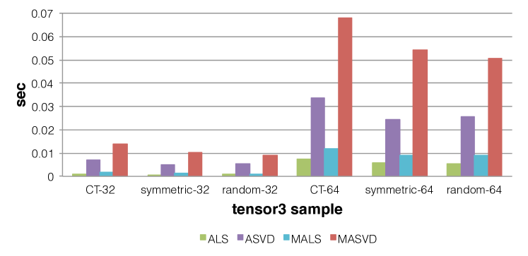
(a) CPU time (s) for medium sized 3-mode tensor samples

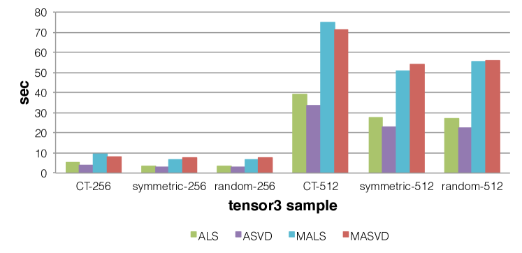
(b) CPU time (s) for larger 3-mode tensor samples

Figure 1: Average CPU times for best rank one approximations per algorithm and per data set taken over 10 different initial random guesses.

Furthermore, we compared the number of optimization calls needed for the algorithms of ALS, ASVD, MALS, and MASVD, recalling that for the ALS and the MALS, one mode is optimized per optimization call, while for ASVD and MASVD, two modes are optimized per optimization call. Figure 2 demonstrates the relationships of the four algorithms (color encoded) on three different data sets (marker encoded) and the different data set sizes (hue encoded). As can be seen, the ASVD has the smallest number of optimization calls followed by the ALS, the MASVD and the MALS. One notices as well that the number of optimization calls for the two random data sets are close to each other for the respective algorithms. The real data set takes most optimization calls, even though it probably profits from more potential correlations. However, the larger number of optimization calls may also result from the different precision of one element of the third-order tensor (16bit vs. 8bit values). Another explanation might be that it was difficult to find good rank one bases for a real data set (the error is approx. 70% for the $512^{3}$ tensor). For random data, the error stays around 63%, probably due to a good distribution of the random values. Otherwise, the number of optimization calls followed the same relationships as already seen in the timings measured for the rank one approximation algorithm. For data sets larger than $128^{3}$, the time per optimization call stays roughly the same for any of the decomposition algorithms. However, the number of needed optimization calls is largest for the MALS and lowest for the ASVD.

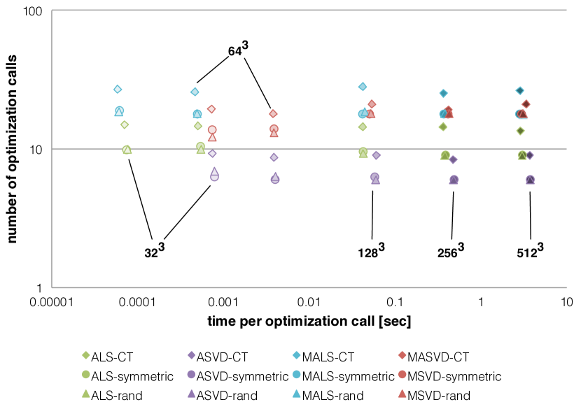
Figure 2: Average time per optimization call put in relationship to the average number of optimization calls needed per algorithm and per data set taken over 10 different initial random guesses.

It is not only important to check how fast the different algorithms perform, but also what quality they achieve. This was measured by checking the Frobenius norm of the resulting decompositions, which serves as a measure for the quality of the approximation. In general, we can say that the higher the Frobenius norm, the more likely it is that we find a global maximum. Accordingly, we compared the Frobenius norms in order to say whether the different algorithms converged to the same stationary point. In Figure 3, we show the absolute differences of the average Frobenius norms achieved by the ALS, ASVD, MALS and MASVD. The differences are taken with respect to the ALS. As previously seen, the results for the real CT data set and the two random dataset differ. For the real data set, the differences for the achieved qualities are much smaller. Moreover, we see that the achieved quality for the ALS and the MALS are almost the same. A similar observation applies to the ASVD and the MASVD, which achieve almost the same quality. We observed that all the algorithms reach the same stationary point for the smaller and medium data sets. However, for the larger data sets ($\geq 128^{3}$) the stationary points differ slightly. We suspect that either the same stationary point was not achieved, or the precision requirement of the convergence criterion was too high. That means that the algorithms stopped earlier, since the results are not changing that much anymore in the case that the precision tolerance for convergence is $0.0001$.

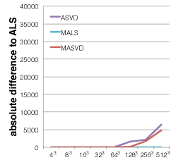
(a) CT data set

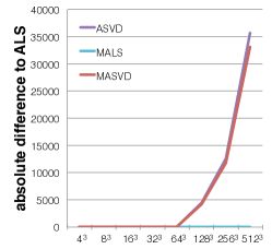
(b) symmetric data set

(c) random data set

Figure 3: Differences of the achieved Frobenius norms by ALS, ASVD, MALS, and MASVD. The Frobenius norm of the approximations per algorithm and per data set are averages taken over 10 different initial random guesses.

Finally, the results of best rank one approximation for symmetric tensors using ALS, MALS, ASVD and MASVD show that the best rank one approximation is also symmetric, i.e., is of the form $a\mathbf{u}\otimes\mathbf{v}\otimes\mathbf{w}$, where $\mathbf{u}\approx\mathbf{v}\approx\mathbf{w}\in\mathrm{S}^{m-1}$. This confirms an observation made by Paul Van Dooren, (private communication), and the main result in [5], which claims that the best rank one approximation of a symmetric tensor can be always chosen symmetric. The results of ASVD and MASVD give a better symmetric rank one approximation, i.e., $\mathbf{u}-\mathbf{v},\mathbf{u}-\mathbf{w}$ in ASVD and MASVD are smaller than in ALS and MALS.

6 Conclusions

We have presented a new alternating algorithm for the computation of the best rank one approximation to a d-mode tensor. In contrast to the alternating least squares method, this method uses a singular value decomposition in each step. In order to achieve guaranteed convergence to a semi-maximal point, we have modified both algorithms. We have run extensive numerical tests to show the performance and convergence behavior of the new methods.

Appendix: Remarks on local semi-maximality

In this appendix we discuss the notion of an isolated critical point of a function $f$ which is semi-maximal but not maximal. The main emphasize is to characterize semi-maximal points for which the alternating maximization iteration, abbreviated as AMI, converges to the critical point at least for some nontrivial choices of the starting points. We explain the convergence issues for ALS on local semi-maximality by the help of the AMI.

Consider a polynomial function $p(\mathbf{t}),\ \mathbf{t}\in\mathbb{R}^{N}$ and let $M\subset\mathbb{R}^{N}$ be a smooth compact manifold of dimension $L$. Denote by $g$ the restriction of $p$ to $M$. For example, in the three mode case we let $N=m+n+l$, $\mathbf{t}=(\mathbf{x},\mathbf{y},\mathbf{z})$, $p(\mathbf{t})=\mathcal{T}\times(\mathbf{x}\otimes\mathbf{y}\otimes\mathbf{z})$ and $M=\mathrm{S}^{m-1}\times\mathrm{S}^{n-1}\times\mathrm{S}^{l-1},\ L=N-3$. Assume that a point $\mathbf{t}_{\star}\in M$ is a non-degenerate critical point of $g$ on $M$. We take local coordinates around $\mathbf{t}_{\star}$, so that in these local coordinates $\mathbf{t}_{\star}$ corresponds to the zero vector of dimension $L$, denoted as $\mathbf{0}_{L}$. So the open connected neighborhood of $\mathbf{t}_{\star}$ is identified with an open connected neighborhood $\mathbf{0}_{L}\in\mathbb{R}^{L}$. Assume that the local coordinates around $\mathbf{0}_{L}$ are $\mathbf{x}^{\top}=[\mathbf{x}_{1}^{\top},\ldots,\mathbf{x}_{d}^{\top}]^{\top},\mathbf{x}_{j}\in\mathbb{R}^{m_{j}},j\in[d]$.

The AMI method consists of maximizing $g$ (or $f$) on $\mathbf{x}_{j}$ for $j=1,\ldots,d$, and then repeating the process. Let us discuss the details of the AMI for a function $f$ given by a quadratic form in the block vector $\mathbf{x}^{\top}=[\mathbf{x}_{1}^{\top},\ldots,\mathbf{x}_{d}^{\top}]\in\mathbb{R}^{L}$, given by

$$f=-\mathbf{x}^{\top}H\mathbf{x},\ H=\left[\begin{array}[]{cccc}H_{1,1}&H_{1,2}&\cdots&H_{1,d}\\ H_{2,1}&H_{2,2}&\ddots&H_{2,d}\\ \vdots&\ddots&\ddots&\vdots\\ H_{d,1}&\cdots&H_{d,d-1}&H_{d,d}\end{array}\right],$$ (6.5)

$$H_{p,q}^{\top}=H_{q,p},\ p,q\in[d].$$

Note that locally we obtain this form for general $f$ via Taylor expansion and leaving off terms of order higher than two.

Consider the AMI iteration $\xi_{k-1}:=[\xi_{1,k-1}^{\top},\ldots,\xi_{d,k-1}^{\top}]^{\top}\to\xi_{k}=[\xi_{1,k}^{\top},\ldots,\xi_{d,k}^{\top}]^{\top}\in\mathbb{R}^{L}$ for a function $f$ of the form (6.5) starting from a point $\xi_{0}$. Then this iteration is the block Gauß-Seidel iteration, see e.g. [17], applied to the linear system $-H\xi=\xi_{0}$ with the block symmetric matrix $H$, i.e.,

$$-\sum_{\ell=1}^{j}H_{j,\ell}\xi_{\ell,k}=\sum_{\ell=j+1}^{d}H_{j,\ell}\xi_{\ell,k-1},\quad j=1,\ldots,d,\quad k\in\mathbb{N}.$$ (6.6)

This iterative method can be expressed as $-L_{H}\xi_{k}=U_{H}\xi_{k-1}$, where $H=L_{H}+U_{H}$ is the decomposition of $H$ into the block lower triangular part $L_{H}$ and the strict block upper triangular part $U_{H}$. Assume that $L_{H}$ is invertible, which is equivalent to the requirement that all diagonal blocks $H_{j,j}$ are invertible. Then (6.6) is of the form $\xi_{k}=K\xi_{k-1}$, where

$$K:=-L_{H}^{-1}U_{H}.$$ (6.7)

It is well known that an iteration $\xi_{k}=K\xi_{k-1}$ will converge to $\mathbf{0}_{L}$ for all starting vectors $\xi_{0}$ if and only if the spectral radius of $K$, denoted as $\rho(K)$, is less than $1$. If $\rho(K)\geq 1$ then the iteration will converge to $\mathbf{0}_{L}$ if and only if $\xi_{0}$ lies in the invariant subspace of $K$ associated with the eigenvalues of modulus less than $1$.

Assume in the following that $\mathbf{0}_{L}:=[\mathbf{0}_{m_{1}}^{\top},\ldots,\mathbf{0}_{m_{d}}]^{\top}$ is a semi-maximal point, i.e., that all diagonal blocks $H_{j,j},\ j\in[d]$ of $H$ are positive definite. Then it follows from a classical result of Ostrowski, see e.g. [17, Thm 3.12], that the iteration (6.6) converges to $\mathbf{0}_{L}$ if and only if $H$ is positive definite, which is equivalent to $\rho(K)<1$. Clearly, in this case $\mathbf{0}_{L}$ is non-maximal for $f(\xi)$ if and only if $H$ is indefinite.

We summarize these observations to give a precise condition on $\xi_{0}$ so that the iteration (6.6) converges to zero, which in the particular case discussed here can be proved easily. We give a proof for completeness.

      Theorem 6

Let $\mathbf{0}_{L}:=[\mathbf{0}_{m_{1}}^{\top},\ldots,\mathbf{0}_{m_{d}}]^{\top}$ be a semi-maximal point of $f(\xi)=-\xi^{T}H\xi$, i.e., each $H_{i,i}$ is positive definite and let $K$ be given by (6.7). Denote by $\alpha,\beta,\gamma$ the number of eigenvalues $\lambda$ of $K$, counting with multiplicities, satisfying $|\lambda|<1,|\lambda|>1,|\lambda|=1$, respectively. Assume that $H$ has $\pi,\nu,\zeta$ positive, negative and zero eigenvalues, respectively. Then

$$\pi\geq\max\{m_{j},j\in[d]\},$$ (6.9)

$$\alpha=\pi,\quad\beta=\nu,\quad\gamma=\zeta.$$

Furthermore, all $\gamma$ eigenvalues of $K$ on the unit circle correspond to a unique eigenvalue $1$ of geometric multiplicity $\gamma$. The corresponding eigenvectors of $K$ are the eigenvectors of $H$ corresponding to the zero eigenvalue.

Proof. We first prove (6.9). Let $H_{i,i}$ be the diagonal block of maximal size $m_{i}$. Let $\tilde{H}$ be a principal submatrix of $H$ of order $m_{i}+1$ which has $H_{i,i}$ as its submatrix. The Cauchy interlacing theorem [10] implies that the eigenvalues of $\tilde{H}$ interlace with the eigenvalues of $H_{i,i}$. Since all eigenvalues of $H_{i,i}$ are positive it follows that $\tilde{H}$ has at least $m_{i}$ positive eigenvalues and hence, (6.9) holds.

To prove (6.9), assume first that $\zeta\geq 1$. But if $\mathbf{x}$ is an eigenvector of $H$ corresponding to the eigenvalue $0$ then $K\mathbf{x}=\mathbf{x}$. Hence $\gamma\geq\zeta$, and $1$ is an eigenvalue of $K$ of geometric multiplicity at least $\zeta$.

Let $\mathbf{V}_{0}$ be the null space of $H$. Then $K$ restricted to $\mathbf{V}_{0}$ is the identity operator. Consider the quotient space $\mathbf{Q}:=\mathbb{R}^{L}/\mathbf{V}_{0}$. Clearly, $K$ and $H$ induce linear operators $K_{1},H_{1}:\mathbf{Q}\to\mathbf{Q}$, where $H_{1}$ is nonsingular with $\pi$ positive eigenvalues and $\nu$ negative eigenvalues. Observe also that if $\mathbf{y},\mathbf{z}\in\mathbb{R}^{L}$ and $\mathbf{y}-\mathbf{z}\in\mathbf{V}_{0}$ then $\mathbf{y}^{\top}H\mathbf{y}=\mathbf{z}^{\top}H\mathbf{z}$. Thus, it is enough to study the eigenvalues of $K_{1}$, which corresponds to the case where $H$ is nonsingular, which we assume from now on.

Observe that the AMI does not decrease the value of $f(\xi)$. Moreover, $f(\xi_{k})=f(\xi_{k-1})$ if and only if $\xi_{k-1}=\mathbf{0}_{L}$. Let us, for simplicity of notation, consider the iteration $\xi_{k}=K\xi_{k-1}$ in the complex setting, i.e., we consider $F(\xi)=-\xi^{*}H\xi$ ,where $\xi\in\mathbb{C}^{L}$. All the arguments can also be carried out in the real setting, by considering pairs of complex conjugate eigenvalues and the corresponding real invariant subspace associated with the real and imaginary part of an eigenvector.

Let $\lambda$ be an eigenvalue of $K$ and let $\xi_{0}$ be the eigenvector to $\lambda$. Then $F(\xi_{1})=|\lambda|^{2}F(\xi_{0})>F(\xi_{0})$ which implies that $|\lambda|\neq 1$. (This implies that the only eigenvalue of $K$ of modulus $1$ can be the eigenvalue $1$, which corresponds to the eigenvalue $0$ of $H$.)

Observe next, that if $H$ is positive definite, then $F(\xi_{0})<0$ and the inequality $F(\xi_{1})>F(\xi_{0})$ yields that $|\lambda|^{2}<1$, i.e., $\rho(K)<1$, which is Ostrowski’s theorem.

¿From now on we therefore assume that $H$ is indefinite and nonsingular. Assume that $F(\xi_{0})\geq 0$ and $\xi_{0}\neq\mathbf{0}_{L}$. Then $F(\xi_{k})$ is an increasing sequence which either diverges to $+\infty$ or converges to a positive number. Hence we cannot have convergence $\xi_{k}\to\mathbf{0}_{L}$. More precisely, we have convergence $\xi_{k}\to\mathbf{0}_{L}$ if and only if $F(\xi_{k})\leq 0$ for all $k\geq 0$.

Let $\mathbf{U}_{0}\subseteq\mathbf{U}_{1}\subset\mathbb{C}^{L}$ be the invariant subspaces of $K$ corresponding to the eigenvalues $0$ and the eigenvalues $\lambda$ of modulus less than $1$ of $K$, respectively. So $K\mathbf{U}_{0}\subset\mathbf{U}_{0}$ and $K|\mathbf{U}_{0}$ is nilpotent. Let $l_{0}=\dim\mathbf{U}_{0}$. We have that $F(\xi)\leq 0$ for all $\xi\in\mathbf{U}$. Let $\mathbf{V}_{-},\mathbf{V}_{+}\subset\mathbb{C}^{L}$ be the eigen-subspaces corresponding to negative and positive eigenvalues of $H$, respectively. So $\pi=\dim\mathbf{V}_{+},\nu:=\dim\mathbf{V}_{-}$ and $\pi+\nu=L$. Consider $\mathbf{W}=\mbox{\rm Range}\ (K^{L})$. Then

$$\mathbf{U}_{0}\cap\mathbf{W}=\{\mathbf{0}_{L}\},\;\dim\mathbf{W}=L-l_{0},\;K\mathbf{W}=\mathbf{W},\;\mathbf{W}+\mathbf{U}_{0}=\mathbb{C}^{L}.$$

With $\mathbf{W}_{+}:=\mathbf{W}\cap\mathbf{V}_{+}$, then we have that $\dim\mathbf{W}_{+}\geq\pi-l_{0}$ and $K_{1}:=K|\mathbf{W}$ is invertible. Setting $\mathbf{W}_{j}=K_{1}^{-j}W_{+}$, we have that $\xi_{j}\in\mathbf{W}_{j}$, and $F(K^{k}\xi_{j})\leq 0$ for $k=0,\ldots,j$, and clearly, $\dim\mathbf{W}_{j}=\dim\mathbf{W}_{+}$. Since the space of $\dim\mathbf{W}_{+}$ subspaces in $\mathbb{C}^{L}$ is compact, there exists a subsequence of $\mathbf{W}_{j_{k}},k\in\mathbb{N}$ which converges to a $\dim\mathbf{W}_{+}$ dimensional subspace $\mathbf{X}\subset\mathbb{C}^{L}$. This subspace corresponds to the invariant subspace of $K$ associated with eigenvalues satisfying $0<|\lambda|<1$, since $F(K^{k}\xi)\leq 0$ for all $k\geq 0$ and $\xi\in\mathbf{X}$. Thus, $\mathbf{X}\cap\mathbf{U}_{0}=\{\mathbf{0}_{L}\}$ and $\mathbf{U}_{1}=\mathbf{X}+\mathbf{U}_{0}$. Note that $\dim\mathbf{U}_{1}=\dim\mathbf{X}+\dim\mathbf{U}_{0}\geq\pi$. Since $F(\xi)\leq 0$ for each $\xi\in\mathbf{U}_{1}$ ,it follows that $\dim\mathbf{U}_{1}=\pi$, i.e., $\alpha=\pi$.

As $\alpha+\beta=L$, it then follows that $\beta=L-\alpha=L-\pi=\nu$. $\Box$

As an example, if we apply the ALS method for finding the maximum of the trilinear form $\mathcal{T}\times(\mathbf{x}\otimes\mathbf{y}\otimes\mathbf{z})$ restricted to $(\mathbf{x},\mathbf{y},\mathbf{z})\in M=\mathrm{S}^{m-1}\times\mathrm{S}^{n-1}\times\mathrm{S}^{l-1}$, then this is just the AMI for the local quadratic form $g$. It is well known that $g$ may have several critical points, some of whom are strict local maxima and local semi-maxima see [3, Example 2, p. 1331]. The above analysis shows that the ALS may converge to each of these points for certain appropriate starting points. For a specific $\mathcal{T}\in\mathbb{R}^{m\times n\times l}$ one can expect that the ALS iteration exhibits a complicated dynamics. Hence, it is quite possible that in some cases the ALS method will not converge to a unique critical point, see also [3, 12, 13].

References

• [1] D. Cartwright, B. Sturmfels, The number of eigenvectors of a tensor, arXiv:1004.4953.
• [2] L. de Lathauwer, B. de Moor and J. Vandewalle. A multilinear singular value decomposition. SIAM J. Matrix Anal. Appl. 21 (2000), 1253–1278.
• [3] L. de Lathauwer, B. De Moor and J. Vandewalle, On the best rank-1 and rank-$(R_{1},R_{2},\ldots,R_{N})$ approximation of higher-order tensors, SIAM J. Matrix Anal. Appl. 21 (2000), 1324- 1342.
• [4] S. Friedland, Matrices, http://homepages.math.uic.edu/ friedlan/bookm.pdf
• [5] S. Friedland. Best rank one approximation of real symmetric tensors can be chosen symmetric, arXiv:1110.5689.
• [6] S. Friedland and V. Mehrmann, Best subspace tensor approximations, arXiv:0805.4220v1.
• [7] S. Friedland and G. Ottaviani, The number of singular vector tuples and uniqueness of best rank one approximation of tensors, in preparation.
• [8] G.H. Golub and C.F. Van Loan. Matrix Computations. John Hopkins Univ. Press, Baltimore, Md, USA, 3rd Ed., 1996.
• [9] C.J. Hillar and L.-H. Lim. Most tensor problems are NP hard, arXiv:0911.1393.
• [10] R.A. Horn and C.R. Johnson, Matrix Analysis, Cambridge University Press, Cambridge, UK, 1985.
• [11] T. Kolda. On the best rank-$k$ approximation of a symmetric tensor. Presentation at the XVII Householder Symposium, Tahoe City, 2011.
• [12] T.G. Kolda and B.W. Bader. Tensor decompositions and applications. SIAM Review 51 (2009), 455- 500.
• [13] P.M. Kroonenberg and J. De Leeuw, Principal component analysis of three-mode data by means of alternating least squares algorithms, Psychometrika, 45 (1980), 69 -97.
• [14] L.-H. Lim. Singular values and eigenvalues of tensors: a variational approach. Proc. IEEE International Workshop on Computational Advances in Multi-Sensor Adaptive Processing (CAMSAP ’05), 1 (2005), 129–132.
• [15] L.R. Tucker. Some mathematical notes on three-mode factor analysis. Psychometrika 31 (1966), 279–311.
• [16] vmmlib: A Vector and Matrix Math Library, http://vmmlib.sf.net
• [17] R.S. Varga. Matrix Iterative Analysis. 2nd. ed., Springer Verlag, Berlin, 2000.
• [18] T. Zhang and G.H. Golub. rank one approximation to high order tensors. SIAM J. Matrix Anal. Appl. 23 (2001), 534 -550.