Geodesic Structure of Test Particle in Bardeen Spacetime

Abstract

The Bardeen model describes a regular space-time, i.e. a singularity-free black hole space-time. In this paper, by analyzing the behavior of the effective potential for the particles and photons, we investigate the time-like and null geodesic structures in the space-time of Bardeen model. At the same time, all kinds of orbits, which are allowed according to the energy level corresponding to the effective potentials, are numerically simulated in detail. We find many-world bound orbits, two-world escape orbits and escape orbits in this spacetime. We also find that bound orbits precession directions are opposite and their precession velocities are different, the inner bound orbits shift along counter-clockwise with high velocity while the exterior bound orbits shift along clockwise with low velocity.

I Introduction

The Bardeen model describes a regular space-time Bardeen ; Borde using the energy-momentum tensor of nonlinear electrodynamics as the source of the field equations and it is also known as a regular black-hole solution which obeys the weak energy condition. This global regularity of black hole solutions is quite important to understand the final state of gravitational collapse of initially regular configurations. When ratio of mass to charge is $27g^{2}\leqslant 16m^{2}$, the Bardeen model represents a black hole and a singularity-free structure Eloy1 . When $27g^{2}=16m^{2}$, the horizons shrink into a single one, which corresponds to an extreme black hole such as the extreme Reissner-Nordström solution. The physically reasonable source for regular black hole solution to Einstein equations has been reported around 1998 Eloy2 ; Eloy3 ; Eloy4 ; Magli . In the Bardeen model, the parameter $g$ representing the magnetic charge of the nonlinear self-gravitating monopoleEloy1 , was studied later on.

It is well known that many effects, such as bending of light, gravitational time-delay, gravitational red-shift and precession of planetary orbits, were predicted by General Relativity. Because these gravitational effects are very important for theories and observations, many theoretical physics and astrophysics are interested in investigating them for different gravitational systems. The geodesic structure with a positive cosmological constant was investigated by Jaklitsch et al.Jaklitsch , the corresponding effective potential was analyzed in detail. The analysis of the effective potential for null geodesics in the Reissner-Nordström-de Sitter and Kerr-de Sitter space-time was carried out in Refs. Stuchlik and Jiao . All possible geodesic motions in the extreme Schwarzschild-de Sitter space-time were investigated by Podolsky Podolsky . Lake investigated light deflection in the Schwarzschild-de Sitter space-timeLake . Exact solutions in closed analytic form for the geodesic motion in the Kottler space-time were considered by Kraniotis et al Kraniotis1 . Kraniotis Kraniotis2 investigated the geodesic motion of a massive particle in the Kerr and Kerr (anti)de Sitter gravitational field by solving the Hamilton acobi partial differential equation. Cruz et al.Cruz studied the geodesic structure of the Schwarzschild anti-de Sitter black hole. Chen and Wang chen1 ; chen2 ; chen3 ; chen4 have investigated the orbital dynamics of a test particle in gravitational fields with an electric dipole and a mass quadrupole, and in the extreme Reissner-Nordström black hole spacetime. The motion of test particle in Ho$\breve{r}$ava-Lifshitz black hole space-times was studied using numerical techniques Enolskii .

To find all of the possible orbits which are allowed by the energy levels for time-like and null geodesic in Bardeen spacetime, we analysis the effective potentials in detail. To describe the trajectories of massive and null particles, we have a direct visualization of the allowed motions. This paper is organized as follows: In Section II, we give a brief review on the Bardeen spacetime. In Section III, we give out the motion equations, and define the effective potential. In Section IV and V, we discuss the time-like and null geodesic structure of the Bardeen spacetime in detail. A conclusion is given in the last section.

II The Bardeen spacetime

The line element representing the Bardeen spacetime is given byBorde

$$ds^{2}= - [1-\frac{2mr^{2}}{(r^{2}+g^{2})^{\frac{3}{2}}}]dt^{2}+[1-\frac{2mr^{2}}{(r^{2}+g^{2})^{\frac{3}{2}}}]^{-1}dr^{2}$$ (1)

$$+ r^{2}(d\theta^{2}+sin^{2}\theta d\phi^{2}),$$

where the parameter g represents the magnetic charge of the nonlinear self-gravitating monopoleEloy1 . The corresponding lapse function is

$$f(r)=1-\frac{2mr^{2}}{(r^{2}+g^{2})^{\frac{3}{2}}}.$$ (2)

The Bardeen model describes a regular space-time for the following inequality:

$$g^{2}\leqslant\frac{16}{27}m^{2}.$$ (3)

When $g^{2}<\frac{16}{27}m^{2}$, there are two horizons in Bardeen spacetime. For the equality $g^{2}=\frac{16}{27}m^{2}$, the horizons shrink into a single one, which are showed in Fig.1 in detail.

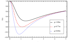
Figure 1: Horizons of the Bardeen spacetime.

III Geodesics equation

It is well known that the Euler-Lagrange equations for the variational problem associated to spacetime metric describes the geodesics. So we set up the corresponding Lagrangian according to Eq.(1)

$$\mathcal{L}=-f(r)\dot{t}^{2}+f(r)^{-1}\dot{r}^{2}+r^{2}(\dot{\theta}^{2}+sin^{2}\theta\dot{\phi}^{2}),$$ (4)

in which the dots denote the derivative with respect to the affine parameter $\tau$. The Hamiltonian motion equations are

$$\dot{\Pi}_{q}-\frac{\partial{\mathcal{L}}}{\partial q}=0,$$ (5)

where $\Pi_{q}=\partial{\mathcal{L}}/\partial\dot{q}$ is the momentum to coordinate $q$. Since the Lagrangian is independent of $(t,\phi)$, the corresponding conjugate momentums are conserved, therefore

$$\Pi_{t}=-(1-\frac{2mr^{2}}{(r^{2}+g^{2})^{\frac{3}{2}}})\dot{t}=-E,$$ (6)

$$\Pi_{\phi}=r^{2}sin^{2}\theta\dot{\phi}=L,$$ (7)

where $E$ and $L$ are motion constants.

From the motion equation for $\theta$

$$\dot{\Pi}_{\theta}-\frac{\partial{\L}}{\partial\theta}=0,$$ (8)

we obtain

$$\frac{d(r^{2}\dot{\theta})}{d\tau}=r^{2}sin\theta cos\theta\dot{\phi}^{2}.$$ (9)

If we simplify the above equation by choosing the initial conditions $\theta=\pi/2$, $\dot{\theta}=0$ and $\ddot{\theta}=0$, the Eq.(7) becomes

$$\Pi_{\phi}=r^{2}\dot{\phi}=L,$$ (10)

from Eqs.(6, 7), the Lagrangian (4) can be written in the following form

$$2{\mathcal{L}}\equiv h=\frac{E^{2}}{1-\frac{2mr^{2}}{(r^{2}+g^{2})^{\frac{3}{2}}}}-\frac{\dot{r}^{2}}{1-\frac{2mr^{2}}{(r^{2}+g^{2})^{\frac{3}{2}}}}-\frac{L^{2}}{r^{2}}.$$ (11)

Now we solve the above equation for $\dot{r}^{2}$ in order to obtain the radial equation, which allows us to characterize possible moments of test particles and explicit solutions of the motion equation of test particles in the invariant plane

$$\dot{r}^{2}=E^{2}-(1-\frac{2mr^{2}}{(r^{2}+g^{2})^{\frac{3}{2}}})(h+\frac{L^{2}}{r^{2}}),$$ (12)

It is useful to rewrite the above motion equation as a one-dimensional problem

$$\dot{r}^{2}=E^{2}-V_{eff}^{2},$$ (13)

where $V_{eff}^{2}$ is defined as an effective potential

$$V_{eff}^{2}=(1-\frac{2mr^{2}}{(r^{2}+g^{2})^{\frac{3}{2}}})(h+\frac{L^{2}}{r^{2}}).$$ (14)

IV Time-like Geodesic Structure

For time-like geodesic $h=1$, the corresponding effective potential becomes

$$V_{eff}^{2}=(1-\frac{2mr^{2}}{(r^{2}+g^{2})^{\frac{3}{2}}})(1+\frac{L^{2}}{r^{2}}).$$ (15)

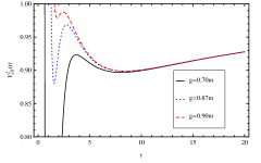
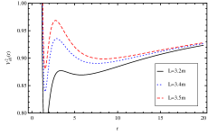
Figure 2: The behavior of the effective potential of non-radial particle for fixed $L=3.5m$(left) and fixed $g=0.87m$(right).

and the orbit equation for massive particle is

$$\dot{r}^{2}=E^{2}-(1-\frac{2mr^{2}}{(r^{2}+g^{2})^{\frac{3}{2}}})(1+\frac{L^{2}}{r^{2}}).$$ (16)

By using Eq.(10) and making the change of variable $u^{-1}=r$, we can obtain orbit equation for massive particle

$$(\frac{du}{d\phi})^{2}=\frac{E^{2}-1}{L^{2}}-u^{2}+\frac{2mu+2mu^{3}L^{2}}{L^{2}(1+u^{2}g^{2})^{\frac{3}{2}}},$$ (17)

Differentiating (17), we have its second order motion equation

$$\frac{d^{2}u}{d\phi^{2}}+u=\frac{3mu^{2}L^{2}+3m}{L^{2}(1+u^{2}g^{2})^{\frac{5}{2}}}-\frac{2m}{L^{2}(1+u^{2}g^{2})^{\frac{3}{2}}},$$ (18)

We solved (17) and (18) numerically to find all types of geodesics and examine how the parameters influence on the timelike geodesics in the space-time of Bardeen model in detail.

From the effective potential curve (see Fig.3), we can identify 3 classes of orbits: i.e. planetary orbits, escape orbits and circular orbits when the energy of particle $E$ satisfies two critical values $E_{C_{1}}$ and $E_{C_{2}}$.

Figure 3: The behavior of the effective potential in Bardeen space-time with $g=0.70m$, $L=3.5m$, $m=1$ and energy levels $E_{C_{2}}^{2}=0.90$ and $E_{C_{1}}^{2}=0.92$.

IV.1 Time-like bound geodesics

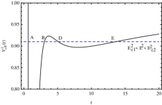
Figure 4: The behavior of the effective potential of time-like bound geodesics for $E^{2}=0.91,g=0.7m,L=3.5m,m=1$

In Fig.4 the dashed line denotes the value of the energy $E^{2}=0.91$, i.e. $E_{C_{1}}^{2}<E^{2}<E_{C_{2}}^{2}$. From potential curve, we can find two kinds of bound orbits for this energy level:

I) The particle orbits on a many-world bound orbit between the range $r_{A}<r<r_{B}$, which is near the singularity and can cross the two event horizons. The $r_{A}$ and $r_{B}$ are the perihelion and aphelion distance of the planetary orbits, respectively. We also can find the clockwise precession of planetary orbits which it is a well-known gravitational effect in general relativity theory.

II) The particle orbit is on a two-world bound orbit in the range $r_{D}<r<r_{E}$, where the $r_{D}$ and $r_{E}$ are the perihelion and aphelion distance, which are larger than the orbit of Case I. The two-world bound orbit is outside the event horizon. However, we also can find that the precession direction of the planetary orbit is counter-clockwise, and the precession velocity is slower than the orbit of Case I.

These two kinds of two-world bound orbits are simulated in Fig.6.

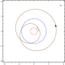
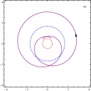
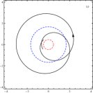
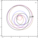
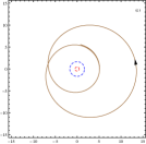
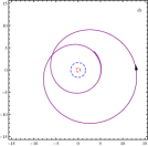
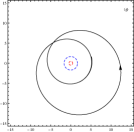
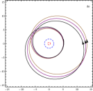
Figure 5: Examples of the two-world bound orbit in the Bardeen space-time with $E^{2}=0.91$, $g=0.7m$, $L=3.5m$ and $m=1$.

IV.2 Time-like circle geodesics

From Fig.6 and 7, we can see that there are two different circular orbits. One is a unstable circular orbit, the other one is a stable circular orbit.

I) When the energy of particle $E$ equals the peak value $E_{C_{2}}$ of the effective potential, the particle can orbit on a unstable circular orbit at $r=r_{C_{2}}$. Any perturbation would make such unstable orbit recede from $r=r_{C_{2}}$ to $r=r_{A}$, then reflect at $r=r_{A}$, or move from $r=r_{C_{2}}$ to $r=r_{B}$, then reflect at $r=r_{B}$. The particle will move between $r=r_{A}$ and $r=r_{B}$ and will make a unstable choice on a movement direction due to the perturbation. Figure 6 shows two cases numerically.

II) When the energy of particle $E$ equals the bottom value $E_{C_{1}}$ of the effective potential, the particle can orbit on a stable circular orbit at $r=r_{C_{1}}$. Or the particle orbits on a many-world bound orbit in the range $r_{A}<r<r_{D}$, where the $r_{A}$ and $r_{D}$ are the perihelion and aphelion distance, respectively. Figure 7 shows two cases numerically.

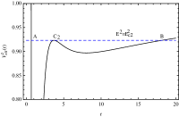
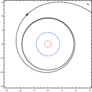
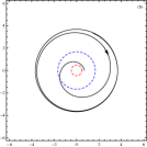
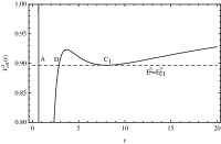
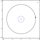
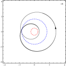
Figure 6: Examples of the unstable time-like circle orbit in the Bardeen space-time with $E_{C_{2}}^{2}=0.92$, $g=0.7m$, $L=3.5m$ and $m=1$.

Figure 7: Examples of the stable time-like circle orbit in the Bardeen space-time with $E^{2}=0.90$, $g=0.7m$, $L=3.5m$ and $m=1$.

IV.3 Time-like escape geodesics

When the particle energy is above the critical value (i.e. the peak value $E_{C_{2}}$ of the effective potential), the particle can orbit on a two-world escape orbit with a curly structure and cross the two horizons which is showed in Fig.8a. When the energy of particle is much higher than the critical value, the escape orbit straightly deflects without curls, which is showed in Fig.8b. This means that the test particle coming from infinite would be reflected at a value of $r$ and would not be able to reach $r=0$, due to the infinite potential barrier at $r=0$. on the other words the particle approaches the black hole from an asymptotically flat region, crosses the horizons twice and moves away into another asymptotically region.

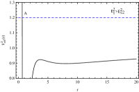
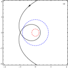
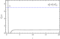
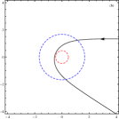
Figure 8: Examples of the two-world escape orbit in the Bardeen space-time with $E_{1}^{2}=1.2$, $g=0.7m$, $L=3.5m$ and $m=1$ (top) and the time-like escape orbit in the Bardeen space-time with $E_{2}^{2}=7$, $g=0.7m$, $L=3.5m$ and $m=1$(bottom).

V Null Geodesics

For the null geodesic $h=0$, we get the corresponding effective potential from Eq.(14)

$$V_{eff}^{2}=(1-\frac{2mr^{2}}{(r^{2}+g^{2})^{\frac{3}{2}}})\frac{L^{2}}{r^{2}}.$$ (19)

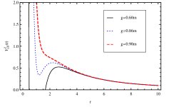
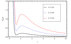
Figure 9: The behavior of the effective potential of the null geodesics for fixed $L=3.5m,m=1(left)$ and for fixed $g=0.8m,m=1(right)$.

The behavior of the effective potential depends on the parameters $g$, $L$ and the corresponding orbit equation is

$$\dot{r}^{2}=E^{2}-(1-\frac{2mr^{2}}{(r^{2}+g^{2})^{\frac{3}{2}}})\frac{L^{2}}{r^{2}}.$$ (20)

By using Eq.(20) and making the change of variable $u^{-1}=r$, we obtain the orbit equation for massive particle

$$(\frac{du}{d\phi})^{2}=\frac{E^{2}}{L^{2}}-u^{2}(1-\frac{2mu}{(1+u^{2}g^{2})^{\frac{3}{2}}}).$$ (21)

By differentiating the Eq.(21), we have

$$\frac{d^{2}u}{d\phi^{2}}+u=\frac{3mu^{2}}{(1+u^{2}g^{2})^{\frac{5}{2}}}.$$ (22)

We must solve the geodesic equations (21) and (22) numerically to investigate the null geodesics structure and how the space-time parameters influence on the null geodesics structures in the Bardeen spacetime. We continue to follow the similar process of the Section IV.

V.1 Null bound geodesics

From the effective potential curve for photons in Fig.10, we can see that there are two different types of orbit when the energy $E$ belows the peak energy value $E_{C}$. When the initial position is between $r_{A}$ and $r_{B}$, the particle will move on a many-world bound orbit with the range of radius from $r_{A}$ to $r_{B}$. When the particle initial position is on the right hand side of the potential barrier, the particle approaches $r_{D}$ from an asymptotically flat region, then will be reflected to move away into another asymptotically region. These two kinds of orbits corresponding to the energy level are plotted on the right side of Fig.10, respectively.

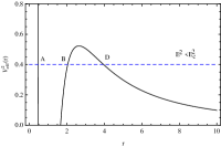
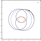
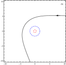
Figure 10: Examples of of the many-world null bound and escape geodesics in Bardeen spacetime with $E^{2}=0.4$, $g=0.6m$, $L=3.5m$ and $m=1$.

V.2 Null circle geodesics

When the energy $E=E_{C}$, The photon can orbit on a unstable circular orbit at $r=r_{C}$, and the photo on such orbit will more likely recede from $r_{C}$ to $r_{A}$ crossing the horizons and will be reflected at $r_{A}$ or escape to the infinity on the other side of the potential barrier due the initial conditions and outside perturbation. Examples of such two kinds of orbits are shown in Fig.11.

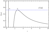
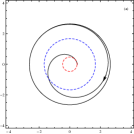
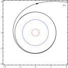
Figure 11: Examples of of two kinds of unstable null circle geodesics in Bardeen spacetime with $E^{2}=0.52$, $g=0.6m$, $L=3.5m$ and $m=1$.

V.3 Null escape geodesics

When the energy $E>E_{C}$, The photon will be on the three different kinds of the escape geodesics which are shown in Fig.12. We can see that when the energy level becomes larger from 0.6 to 7, the corresponding orbit changes from the two-world escape orbit to the escape orbit without intersection point. this means the particle approaches the black hole from an asymptotically flat region, crosses the horizons and then moves away into another asymptotically region.

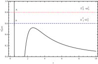
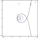
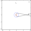
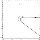
Figure 12: Examples of three kinds of null escape geodesics in Bardeen spacetime with $g=0.6m$, $L=3.5m$, $m=1$ and two energy levels $E_{1}^{2}=0.6$ and $E_{2}^{2}=0.8$.

VI conclusions

By analyzing the effective potential of massless and massive test particles in the Bardeen space-time, which describes a regular space-time and also represents a singularity free black hole for $g^{2}<(16/27)m^{2}$, where the parameter $g$ represents the magnetic charge of the nonlinear self-gravitating monopole, and numerically simulating all possible orbits corresponding to all kinds of energy levels, we have found that there exist two kinds of bound orbits, one is close to the center of the black hole and crosses the two horizons, the other is outside the exterior horizon. The interesting result is that the planetary orbital precession direction is opposite and heir precession velocities are different, the inner bound orbit shifts along counter-clockwise with higher velocity while the exterior bound orbit shifts along clockwise with low velocity, as shown in Fig.5. We have also found two kinds of circular orbits, the inside one which closes to the exterior horizon is unstable and the outside one is a stable circular orbits, and two kinds of escape orbits. For the photon particle, there only exist one many-world bound orbit which can cross the inner- and out-horizons, one unstable circular orbit and three kinds of escape orbits.

VII Acknowledgments

This project is supported by the National Natural Science Foundation of China under Grant No.10873004, the State Key Development Program for Basic Research Program of China under Grant No.2010CB832803 and the Program for Changjiang Scholars and Innovative Research Team in University, No. IRT0964.

References

- (1) J. Bardeen, presented at GR5, Tiflis, U.S.S.R., and published in the conference proceedings in the U.S.R. (1968).
- (2) A. Borde, Phys. Rev. D. 55, 7615 (1997).
- (3) E. Ayón-Beato and A. García, Phys. Lett. B. 493, 149 (2000).
- (4) E. Ayón-Beato and A. García, Phys. Rev. Lett. 80, 5056 (1998).
- (5) E. Ayón-Beato and A. García, Gen. Rel. Gravit. 31, 629 (1999).
- (6) E. Ayón-Beato and A. García, Phys. Lett. B. 464, 25 (1999).
- (7) G. Magli, Rept. Math. Phys. 44, 407 (1999).
- (8) M. J. Jaklitsch, C. Hellaby and D. R. Matravers, Gen. Rel. Grav. 21, 94 (1989).
- (9) Z. Stuchlik and M. Calvani, Gen. Rel. Grav. 23, 507 (1991).
- (10) J. Podolsky, Gen. Rel. Grav. 31, 1703 (1999).
- (11) Z. Y. Jiao and Y. C. Li, Chin. Phys. 11, 467 (2002).
- (12) K. Lake, Phys. Rev. D 65, 087301 (2002).
- (13) J. H. Chen and Y. J. Wang, Class. Quantum. Grav. 20, 3897 (2003).
- (14) G. V. Kraniotis and S. B. Whitehouse, Class. Quantum. Grav. 20, 4817 (2003).
- (15) G. V. Kraniotis, Class. Quantum Grav. 21, 4743 (2004)
- (16) N. Cruz, M. Olivares and J. R. Villanueva, Class. Quant. Grav. 22, 1167 (2005).
- (17) J. H. Chen and Y. J. Wang, Chin. Phys. 15, 1705 (2006).
- (18) J. H. Chen and Y. J. Wang, Chin. Phys. 16, 3212 (2007).
- (19) J. H. Chen and Y. J. Wang, Int. J. Mod. Phys. A. 25, 1439 (2010).
- (20) V. Z. Enolskii, B. Hartmann, and V. Kagramanova, et al. Phys. Rev. D 84, 084011 (2011)