Memory-Constrained Algorithms for Simple Polygons

Abstract

A constant-work-space algorithm has read-only access to an input array and may use only $O(1)$ additional words of $O(\log n)$ bits, where $n$ is the input size. We show how to triangulate a plane straight-line graph with $n$ vertices in $O(n^{2})$ time and constant work-space. We also consider the problem of preprocessing a simple polygon $P$ for shortest path queries, where $P$ is given by the ordered sequence of its $n$ vertices. For this, we relax the space constraint to allow $s$ words of work-space. After quadratic preprocessing, the shortest path between any two points inside $P$ can be found in $O(n^{2}/s)$ time.

1 Introduction

In algorithm development and computer technology, we observe two opposing trends: on the one hand, there are vast amounts of computational resources at our fingertips. Alas, this often leads to bloated software that is written without regard to resources and efficiency. On the other hand, we see a proliferation of specialized tiny devices that have a limited supply of memory or power. Software that is oblivious to space resources is not suitable for such a setting. Moreover, even if a small device features a fairly large memory, it may still be preferable to limit the number of write operations. For one, writing to flash memory is slow and costly, and it also reduces the lifetime of the memory. Furthermore, if the input is stored on a removable medium, write-access may be limited for technical or security reasons.

With this situation in mind, it makes sense to focus on algorithms that need only a limited amount of work-space, while the input resides in read-only memory. In this paper, we will develop such algorithms for geometric problems in planar polygons or, more generally, plane straight-line graphs (PSLGs).

In particular, we consider two fundamental problems from computational geometry [6]: first, we are given a PSLG $G=(V,E)$ with $n$ vertices, and we would like to find a triangulation for $G$, i.e., a PSLG with vertex set $V$ that contains all the edges in $E$ and to which no edge can be added without violating planarity. We show how to find such a triangulation in $O(n^{2})$ time with $O(1)$ words of work-space (Section 4). Since our model does not allow storing the output, our algorithm outputs the triangles of the triangulation one after another.

Then, we apply this result in order to construct a memory-adjustable data structure for shortest path queries in simple polygons (Section 5). Given a simple polygon $P$ with $n$ vertices and a parameter $s\in\{1,\ldots,n\}$, we build a data structure for $P$ that requires $O(s)$ words of storage and that lets us output the edges of a shortest path between any two points inside $P$ in $O(n^{2}/s)$ time using $O(s)$ work-space. The preprocessing time is $O(n^{2})$.

Model Assumptions.

The input to our algorithms is either a simple polygon $P$ or a PSLG $G$ with $n$ vertices, stored in a read-only data structure. In case of a PSLG, we assume that $G$ is given in a way that allows us to enumerate all edges of $G$ in $O(n)$ time and to find the incident vertices of a given edge in constant time (a standard adjacency list representation will do). In case of a polygon, we require that the vertices of $P$ are stored according to their counterclockwise order along the boundary, so that we can obtain the (clockwise and counterclockwise) neighbor of any given vertex in constant time. We also assume that is takes constant time to access the $x$- and $y$-coordinates of any vertex and to perform basic geometric operations, such as determining whether a point lies above or below a given line.

Storage is counted in terms of cells or words. As usual, a word is assumed to be large enough to contain either an input item (such as a point coordinate) or a pointer into the input structure (of $\Theta(\log n)$ bits). Thus, in order to convert our storage bounds into bits, we have to multiply them by a factor of $\log n$. In addition to the input, which can only be read, the algorithm has $O(s)$ words of work-space at its disposal for reading and writing. Here, $s$ is a parameter of the model and can range between $1$ and $n$. We will consider both the case where $s$ is a fixed constant and the case where $s$ can be chosen by the user. Since there is no way to store the result, we use an additional operation output in order to generate output data. We require that every feature of the desired structure is output exactly once.

For simplicity, we will make the usual general position assumption: no three input vertices are on a line and no two input vertices have the same $x$-coordinate.

Related Work.

Given the many applications of memory-constrained algorithms, a significant amount of research has been devoted to them, even as early as in the 1980s [22]. One of the most studied problems in this setting is that of selection in an unsorted array with elements from a totally ordered universe [23, 22, 18, 25, 11].

In computational complexity theory, the constant-work-space model is represented by the complexity class LOGSPACE [1]. There are several algorithmic results for this class, most prominently Reingold’s celebrated method for finding a path between two vertices in an undirected graph [26]. However, complexity theorists typically do not try to optimize the running time of their constant-work-space algorithms, whereas one of our objectives is to solve a given problem as quickly as possible under the memory constraint.

There are other models that allow only read-access to the input, such as the streaming model [24] or the multi-pass model [10]. In these models, the input can be read only a bounded number of times in sequential order, whereas we allow the input to be accessed in any order and as often as necessary. Other memory-constrained models are succinct data structures [21] and in-place algorithms [9, 8, 12, 7]. The aim of succinct data structures is to use the minimum number of bits to represent a given input. Although this kind of approach significantly reduces the memory requirement, in many cases $\Omega(n)$ bits are still necessary. For in-place algorithms, we also assume that only $O(1)$ cells of work-space are available. However, in this model we are allowed to reorder and sometimes rewrite the input data. This makes it possible to encode our data structures through appropriate permutations of the input and often to achieve the best possible running time. Several classic geometric problems, such as convex hull computation or nearest-neighbor search, have been considered in this model [9, 8, 12, 7]. Note that the improved running times in the in-place model come at the expense of requiring more powerful operations from the computational environment, making the results less widely applicable. Moreover, in most of these cases the input values cannot be recovered after the algorithm is executed.

A classic algorithm from computational geometry that fits into our model is the gift-wrapping method (also known as Jarvis’ march): given $n$ points in the plane, we can report the $h$ points on the convex hull in $O(n{h})$ time using $O(1)$ cells of work-space [27]. More recently, Asano et al. [3] initiated the systematic study of constant-work-space algorithms in a geometric context. They describe algorithms to compute well-known geometric structures (such as the Delaunay triangulation, the Voronoi diagram, and the Euclidean minimum spanning tree) using $O(1)$ cells of work-space. They also show how to obtain a triangulation of a planar point set and how to find the edges of the shortest path between any two points inside a simple polygon. These algorithms use constant work-space and run in quadratic time. We emphasize once again that since the output may have linear size, it is not stored, but reported piece by piece. Recently, Barba et al. [5] gave a constant-work-space algorithm for computing the visibility region of a point inside a simple polygon.

Although we know of no previous method to triangulate a given simple polygon $P$ with sublinear work-space, it is known how to find an ear of $P$ in linear time and constant space [16] (an ear is a triangle inside $P$ defined by a single line segment between two vertices of $P$). However, due to the limited work-space, there seems to be no easy way to extend this method in order to obtain a complete triangulation of $P$.

2 Preliminaries

We start by describing two simple operations and a basic spatial decomposition technique that will be useful in designing our algorithms

Angular and Translational Sweep.

Let $s$ be a point in the plane, and let $r$ be a ray with initial point $t\in r$ such that the line segment $st$ does not intersect any edge of the input PSLG $G$. In an angular sweep, we move $t$ along $r$, and we would like to determine the first vertex of $G$ that is hit by the line segment $st$. Note that the angular sweep is very similar to what is commonly called a gift wrapping query. A translational sweep is similar, but now we have a second ray $r^{\prime}$ with initial point $s$, and the segment $st$ is swept vertically, while maintaining the endpoints on $r$ and $r^{\prime}$. Figure 1 depicts an example of both sweep types. In both cases, the first vertex of $G$ that is hit by $st$ can be found in $O(n)$ time: we only need to check for each vertex whether it lies in the swept area and to maintain the point of smallest angle or of smallest horizontal distance, respectively.

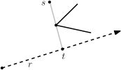
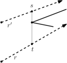
(a)		(b)

Figure 1: Illustration of an angular sweep (a) and a translational sweep (b).

Vertical Decomposition.

The vertical decomposition (or trapezoidation) of $G$ is obtained by shooting vertical rays upward and downward from each vertex of $G$ until they hit another edge of $G$ (or extend to infinity) [6]. This gives a decomposition of the plane into trapezoidal cells. In general position, there are at most two vertices of $G$ on the boundary of each cell. (If $G$ represents a simple polygon $P$, we may be interested only in the trapezoids interior to $P$.)

In our model, the trapezoids incident to a given vertex $p$ can be determined easily in $O(n)$ time per trapezoid [3, 4]: first, we enumerate the edges of $G$ to find the first edge hit by the upward and the downward vertical ray from $p$ in $O(n)$ time. Then, we enumerate all edges incident to $p$ in circular order, including the upward and the downward vertical ray. For each pair of consecutive edges, we perform an appropriate translational sweep to find the trapezoid that is bounded by them. This takes $O(n)$ time per edge.

3 Triangulating a Mountain

In the next section, we will present an algorithm for triangulating an arbitrary PSLG. First, however, we need to explain how to handle inputs of a special kind. The algorithm from this section will serve as an important building block for the general case.

Let $H$ be a simple polygon with vertices $a_{1},a_{2},\dots,a_{k}$, in circular order. We call $H$ a monotone mountain (or mountain for short) if the $x$-coordinates of $a_{1},a_{2},\dots$ increase monotonically. The edge $a_{1}a_{k}$ is called the base of $H$. The shortest path between two points $s$ and $t$ in $H$ is the shortest polygonal chain with endpoints $s$ and $t$ that does not cross the boundary of $H$. We define the shortest path tree SPT as the union of all shortest paths from $a_{1}$ to the other vertices of $H$, see Figure 2. SPT is a rooted tree with root $a_{1}$, and it has the following properties:

Proposition 3.1.

Any two adjacent edges of SPT form a left turn (wrt. $a_{1}$); i.e., SPT bends only “upwards”. Let $f$ be an interior face of the PSLG formed by SPT and $H$. Then (i) $f$ is bounded by the shortest paths from $a_{1}$ to two consecutive vertices $a_{i}$ and $a_{i+1}$; (ii) $f$ is a pseudotriangle, bounded from below by an SPT edge $ua_{i+1}$, from the right by an edge $a_{i}a_{i+1}$ of $H$, and from above by a concave chain of SPT edges (as seen from inside); and (iii) $f$ can be triangulated uniquely by connecting the rightmost vertex $a_{i+1}$ with the reflex vertices on the upper boundary.∎

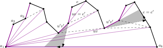
Figure 2: The shortest path tree SPT from $a_{1}$ to all other vertices (in purple). Additional triangulation edges generated in our algorithm are dashed. The figure illustrates a forward step (right shaded area) and a backward step (middle area).

The idea now is to generate the triangulation during a depth-first traversal of the edges of SPT, starting from the base edge $a_{1}a_{k}$ and visiting the children of each vertex in counterclockwise order. This traversal can be interpreted geometrically as an Euler tour of the plane graph SPT. Since there is no space for a stack, this tour must be performed in a “stateless” manner, using angular sweeps to determine the next edge to be traversed. We call a vertex finished if it has been visited by the tour and will not be visited again. Otherwise, the vertex is unfinished. In an Eulerian traversal of SPT, the vertices of $H$ become finished in order from right to left.

Our algorithm maintains two edges: (i) the current edge of the tour $uv$, with $v$ lying to the right of $u$; and (ii) the edge $e=a_{i}a_{i+1}$ of $H$ such that $\{a_{i+1},a_{i+2}\ldots,a_{k}\}$ are the finished vertices of the tour. Observe that we can use $e$ to distinguish between vertices that are finished and those that are not. In each step we distinguish three different cases, and we accordingly perform a step as follows.

Case 1: $v$ is not incident to $e$. We perform a forward step into the subtree rooted at $v$.

Case 2: $v=a_{i}$, but $uv$ is a chord of $H$. We perform a sideways step to the next edge out of $u$ that follows $uv$ in counterclockwise order.

Case 3: $v=a_{i}$, and $uv$ is the edge $a_{i-1}a_{i}$ of $H$. We do a backward step and return to the parent of $u$.

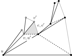
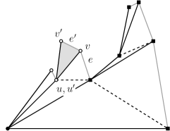
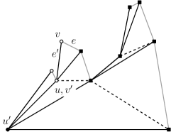
forward step	sideways step	backward step

Figure 3: The three cases for the Eulerian traversal of SPT. The triangles that are reported while performing a step are shaded. Edges in the triangulation that are not contained in SPT are drawn dashed.

We start the algorithm with a sideways step from $uv:=e:=a_{1}a_{k}$ (as an exception to the above rules). The algorithm continues until all vertices are finished and it tries to make a backward step from $e=a_{1}a_{2}$. The details of the three steps are straightforward. In each step, we determine the values $u^{\prime}$, $v^{\prime}$ and $e^{\prime}$ for the next step, and we output some triangles of the triangulation (see Fig. 3; see also Fig. 2 for the forward and the backward step).

Forward step. Let $x$ be the intersection of the line $\overline{uv}$ with the edge $e$. We perform a counterclockwise angular sweep of the segment $vx$ around the vertex $v$, letting $x$ move along $e=a_{i}a_{i+1}$ (By Proposition 3.1, SPT makes only upward bends, so the line $\overline{uv}$ intersects $e$ and the segment $vx$ lies inside $H$). Let $z$ be the first vertex hit by the sweep (note that $z$ might be $a_{i}$). Since $z$ is the first child of $v$, we update $u^{\prime}v^{\prime}:=vz$, leave $e^{\prime}:=e$ and output the triangle $vv^{\prime}a_{i+1}$ (by Proposition 3.1(iii)).

Sideways step. Since $a_{i}$ is now finished, we proceed to the previous edge $e^{\prime}:=a_{i-1}a_{i}$. We make a counterclockwise angular sweep of the segment $uv$, around $u$, letting $v$ mode along $e^{\prime}$. Let $z$ be the first vertex that is hit (again, $z$ might be $a_{i-1}$. We set $u^{\prime}v^{\prime}:=uz$ and output the triangle $uvv^{\prime}$ (by Proposition 3.1(iii)).

Backward step. Since $a_{i}$ is now finished, we proceed to the previous edge $e^{\prime}:=a_{i-1}a_{i}=uv$. Let $x$ be the intersection of the line $\overline{uv}$ with the base edge $a_{1}a_{k}$. As before, Proposition 3.1 ensures that $x$ exists. We do a clockwise angular sweep of the segment $ux$ around $u$, keeping $x$ on the base edge. Call the first vertex that is hit $z$. We set $u^{\prime}v^{\prime}:=zu$.

Each edge of SPT is visited at most twice, so there are $O(k)$ steps. Each step involves one angular sweep and some additional processing that takes constant time. Thus, we get

Theorem 3.2.

Let $H$ be a mountain with $k$ vertices. There is an algorithm that does one counterclockwise scan of $H$ and outputs all triangles in a triangulation of $H$. The algorithm needs $O(k)$ angular sweeps and additional processing time $O(k)$ as well as constant work-space.

In particular, we have shown the following.

Corollary 3.3.

Let $H$ be an explicitly given mountain with $k$ vertices. Then we can output all the triangles in a triangulation of $H$ in $O(k^{2})$ time with constant work-space.

Remark.

Our algorithm produces the same triangulation as the classic algorithm for triangulating monotone polygons [19]. This algorithm processes the vertices from left to right, and it maintains a stack that represents the lower convex hull of the vertices $\{a_{1},\ldots,a_{i}\}$ encountered so far. This lower convex hull is also the shortest path from $a_{1}$ to $a_{i}$. When processing the next vertex $a_{i+1}$, the vertices that disappear from the hull are popped from the stack and appropriate triangles between the popped vertices and the new vertex are generated.

The classic algorithm also performs an implicit depth-first traversal of SPT, but in contrast to our approach, the children of a vertex are visited in clockwise order. Even though we can modify this algorithm for constant work-space, it does not perform a single scan of the vertices of $H$, a property that will be crucial in the next section.

4 Triangulating a PSLG

We now describe how to triangulate a PSLG $G$ with $n$ vertices in $O(n^{2})$ time and with constant work-space. Our algorithm only needs $O(n)$ scans over the edges of $G$, and we make no assumptions about the scanning order.

In the usual model of computation, it is well known that $G$ can be triangulated using the vertical decomposition (cf. Chazelle and Incerpi [15]). Since our algorithm follows the same strategy, we briefly review how this works: first, we compute the edges of the convex hull of $G$ and add them to $G$. Then we find the vertical decomposition of the resulting graph, and insert an edge between any two non-adjacent vertices of $G$ that are contained in the same trapezoid (see Fig. 4). Consider the resulting graph $G^{\prime}$ that contains the convex hull edges and the newly inserted edges. All interior faces of $G^{\prime}$ are mountains: since every vertex (except for the left- and the rightmost ones) has at least one edge incident to either side, the faces must be monotone polygons. Suppose there is a face $f$ with vertices on both the upper and the lower boundary. Then there would be a trapezoid with a vertex at the upper and at the lower boundary, and we would have inserted an edge between those vertices, so $f$ cannot exist. Now, we can easily triangulate each face of the resulting graph with an algorithm for triangulating mountains.

In our setting, we cannot explicitly compute the decomposition of $G$. Instead, we enumerate all edges of $G$ and of the convex hull of $G$. Note that convex hull edges can be found in linear time per edge through Jarvis march [27]. For each such edge $e$, we check whether $e$ is the base of a mountain. This is the case if and only if $e$ is incident to more than one trapezoid above it or more than one trapezoid below it. As described in Section 2, this can be checked in linear time. (An inserted chord is never the base of a mountain.) Once the base of a mountain $H$ is at hand, we would like to use Theorem 3.2 to triangulate it. For this, we need to enumerate the vertices of $H$ in counterclockwise order and to perform angular sweeps. The former can be done by enumerating the trapezoids that are incident on one side of $e$, and takes $O(n)$ time per trapezoid (see Section 2). The latter can be done in $O(n)$ time by enumerating the vertices of $G$, because the vertices outside $H$ cannot affect the angular scan. Thus, by Theorem 3.2, it takes $O(nk)$ time to triangulate $H$, where $k$ is the number of vertices in $H$. Since the total size of all mountains is $O(n)$, we get the following result.

Theorem 4.1.

Given a PSLG $G$ with $n$ vertices, we can output all triangles in a triangulation of $G$ in $O(n^{2})$ time with constant work-space.

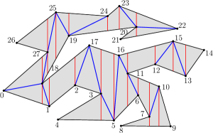
Figure 4: Decomposition of a polygon into mountains.

5 A Memory-Adjustable Data Structure for Shortest Paths

Let $S$ be some set of $n$ objects. In general, the purpose of a data structure $D$ for $S$ is to support certain queries on $S$ efficiently. Ideally, $D$ has linear size, and the query algorithm searches within $D$ with only $O(1)$ cells of additional work-space. In the classic setting, the whole set $S$ is contained in the data structure, so the storage must be at least as large as the input.

We take a different approach: recall that our input cannot be modified. Thus, our strategy is to preprocess the data and to store some additional information in a data structure of size $s$ (for some parameter $s\leq n$). The objective is to design an algorithm that uses this additional information in a way that supports efficient query processing. Ideally, we would like to have a trade-off between the amount of additional storage and the running time of the algorithm. This has been done successfully for many other classic problems such as selection and sorting [23, 25].

Naturally, the most important quality measure for any such algorithm is the query time. However, the preprocessing time for constructing the data structure should also be taken into account. In this section, we describe a data structure for computing the shortest path between any two points inside a simple polygon $P$ with $n$ vertices. It is known that this takes $O(n^{2})$ time with constant work-space [3] and $O(n)$ time with linear work-space [20].

We describe how to construct a data structure that requires $O(s)$ words of storage and that can find the shortest paths between any two points in $P$ in time $O(n^{2}/s)$. The preprocessing time is $O(n^{2})$, and the query algorithm is allowed to use $O(s)$ additional words of work-space. Note that for $s=1$ the query time is $O(n^{2})$, while for $s=n$ the query time is $O(n)$. Thus, we achieve a smooth trade-off between the known results.

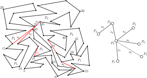
Figure 5: A decomposition of a simple polygon into $7$ disjoint subpolygons using $6$ chords and its associated tree decomposition.

5.1 Preprocessing

During the preprocessing phase, we use our allotted space to compute $O(s)$ chords that partition $P$ into $O(s)$ subpolygons with $\Theta(n/s)$ vertices each, see Figure 5. In the following, these chords will be called cut edges. Our data structure stores the subpolygons together with a tree that represents the adjacencies between them. Each subpolygon is represented by the corresponding cut edges and segments of the boundary of $P$, in counterclockwise order. The boundary segments can be described with $O(1)$ storage cells each, by using the index of the first and the last edge. Thus, the total space for the data structure is $O(s)$.

We use the following well-known observation [13], which is based on the fact that any triangulation of a simple polygon dualizes to a tree with $n-2$ nodes and maximum degree $3$.

Proposition 5.1.

Let $P$ be a simple polygon with $n\geq 4$ vertices. Any triangulation of $P$ has a chord that splits $P$ into two subpolygons with at most $\lfloor(2/3)n\rfloor+1\leq(5/6)n$ vertices each. ∎

A chord as in Proposition 5.1 is called a balanced cut.

Theorem 5.2.

Let $P$ be a simple polygon with $n$ vertices. For any $s\leq n$, there exists a set of $O(s)$ chords that are pairwise non-intersecting and that partition $P$ into $O(s)$ subpolygons with $\Theta(n/s)$ vertices each. The chords can be found in $O(n^{2})$ time using constant work-space.

Proof.

We set $t:=\lceil n/s\rceil$. If $t\leq 3$, we simply output a triangulation of $P$. Otherwise, we use Proposition 5.1 iteratively to split $P$ into smaller and smaller subpolygons. In each round, we scan over all pieces computed so far, and for every piece with more than $t$ vertices we find a balanced cut. In the end, each piece has between $t/6$ and $t$ vertices, so we obtain $O(s)$ subpolygons of size $\Theta(n/s)$.

Let $Q$ be a subpolygon with $k$ vertices. We can find a balanced cut for $Q$ in time $O(k^{2})$: triangulate $Q$ using Theorem 3.2. Whenever the algorithm outputs a new chord, we compute the size of the two pieces it cuts, and we remember the one with the most balanced cut. Note that the size of each piece can be computed in $O(k)$ time: the subpolygon $Q$ is represented as a sequence of at most $O(k)$ cut edges or segments of the boundary of $P$, and for each such segment we can determine the relevant size in constant time.

Consider the $r$-th round, and suppose we have $p\leq n$ pieces of size $n_{1},\dots,n_{p}$, where $n_{1}+\dots+n_{p}=n+2p\leq 3n$. By Proposition 5.1, we have $n_{i}\leq t_{r}:=(5/6)^{r}n$ for all $i$. Thus, the running time for round $r$ is proportional to

$$\sum_{i=1}^{p}n_{i}^{2}\leq t_{r}\sum_{i=1}^{p}n_{i}\leq t_{r}\cdot 3n=3\Bigl{(}\frac{5}{6}\Bigr{)}^{r}n^{2}.$$

Summing over all rounds, we get a total running time of $O(n^{2})$, as claimed. ∎

Remark.

Guibas and Hershberger [20] showed that if linear work-space is available, the preprocessing time can be reduced to $O(n)$. For completeness, we briefly sketch their method. First, we triangulate $P$ with Chazelle’s algorithm [14]. Then, we find the cut edges by greedily pruning the tree $T$ that corresponds to the dual graph of the triangulation. Set $t:=\lceil n/s\rceil$. Every vertex of $T$ has a weight, initialized to $1$. In each round, we scan over the leaves of $T$. We remove those leaves whose weight is between $t/3$ and $t+1$ and declare the corresponding edges to be cut edges. Then, we delete the remaining leaves and add their weight to their parents.

In the end, the remaining part may have less than $t/3$ vertices. If so, we remove one cut edge to merge this part with an adjacent one. Since each vertex is visited once, the whole procedure takes linear time.

5.2 Query Algorithm

We now describe the query algorithm. Given two points $p,q\in P$, we would like to find the shortest path $\pi_{pq}$ between them, while taking advantage of the precomputed polygon decomposition. The main idea is to compute a shortest path for each subpolygon with the constant-work space algorithm of Asano et al. [3], and to concatenate the resulting paths. However, additional steps are necessary to deal with edges of $\pi_{pq}$ that cross several subpolygons, so the algorithm gets a bit more involved.

First, let us quickly review the algorithm of Asano et al. [3] (referred to as AMRW from now on). The AMRW-algorithm stores a triple $(v,r_{1},r_{2})$ of points. The point $v$ is a vertex of $\pi_{pq}$, while $r_{1}$ and $r_{2}$ lie on the boundary of $P$ (not necessarily vertices). The triple maintains the invariant that all vertices of $\pi_{pq}$ up to $v$ have been reported. The line segments $vr_{1}$ and $vr_{2}$ cut off a subpolygon $P^{\prime}\subseteq P$ that contains the target $q$. In each step, the algorithm shoots a ray into $P^{\prime}$ that originates at $v$ and that lies inside the visibility cone determined by $vr_{1}$ and $vr_{2}$. The direction of the ray is chosen according to a case distinction whose details we omit. Let $r^{\prime}$ be the point where this ray hits the boundary of $P^{\prime}$. The line segment $vr^{\prime}$ divides $P^{\prime}$ into two parts, and by determining which part contains the target $q$, we can find a new triple $(v^{\prime},r_{1}^{\prime},r_{2}^{\prime})$. This triple either yields a new vertex of $\pi_{pq}$, or it makes $P^{\prime}$ smaller. AMRW show that in either case the ray shooting operation can be charged to a vertex of $P$ in a way where every vertex is charged at most twice. Thus, since each step takes linear time, the total running time is bounded by $O(n^{2})$. Please refer to the original article for further details [3].

Our algorithm uses a similar strategy: it also maintains a triple $(v,r_{1},r_{2})$ of points that fulfills the same invariant, and in each step it shoots a ray to determine the triple for the next step. As long as the triple and the ray are contained in a simple subpolygon of the decomposition, we can just use the previous method without change while achieving the desired speedup. We call this the standard situation. However, if the points of the triple are not contained in the same polygon, or if the ray crosses a cut edge we need to take additional measures in order to quickly update the triple. In this case, the algorithm switches to a different mode, the long-jump situation. We now describe the details.

Initialization.

We start by locating the subpolygons $P_{p}$, $P_{q}$ that contain $p$ and $q$. For this, we shoot upward vertical rays from $p$ and from $q$, and we find the first edge (or cut edge) $e_{p}$ and $e_{q}$ of $P$ that is hit. This takes linear time. Then we determine the subpolygons $P_{p}$ and $P_{q}$ that contain $e_{p}$ and $e_{q}$. If the edge is a cut edge, this is immediate. If not, we go through the description of the subpolygons, and for each edge sequence, we determine in constant time whether it contains $e_{p}$ or $e_{q}$ by comparing indices. This requires $O(s)$ time, since the total boundary of all subpolygons has $O(s)$ pieces.

If $P_{p}=P_{q}$, we apply the constant-work-space method within $P_{q}$ and are done. Otherwise, we take the tree that represents the polygon partition, and we find the path between $P_{p}$ and $P_{q}$. Every edge on that path corresponds to a cut edge that must be crossed by $\pi_{pq}$, in the same order. For any subpolygon $P_{i}$ that is traversed by $\pi_{pq}$, we define the entrance of $P_{i}$ as the cut edge through which $\pi_{pq}$ enters $P_{i}$ and the exit of $P_{i}$ as the cut edge through which $\pi_{pq}$ leaves $P_{i}$. The remaining cut edges are not be crossed by $\pi_{pq}$, so we treat them as obstacles.

We initialize the triple $(v,r_{1},r_{2})$ as in AMRW. Initially, all of $v$, $r_{1}$ and $r_{2}$ are contained in the same subpolygon of $P$, and we call this polygon $P_{\mathrm{curr}}$. Next, the algorithm enters the standard situation.

Standard Situation.

In the standard situation, both endpoints $r_{1}$ and $r_{2}$ are contained in the same polygon $P_{\text{curr}}$. The vertex $v$ does not necessarily lie in $P_{\text{curr}}$, but since the AMRW-algorithm works with the subpolygon $P^{\prime}$ that is cut off by the segments $vr_{1}$ and $vr_{2}$, we only need to deal with the vertices of $P_{\text{curr}}$ and $v$, see Figure 6.

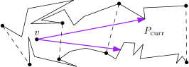
Figure 6: The standard situation.

We apply the AMRW-strategy almost without change: we shoot a ray $R^{\prime}$ that partitions $P_{\text{curr}}$ into two. If $R^{\prime}$ does not hit the exit of $P_{\text{curr}}$, we can use the same rules as in AMRW to update the triple $(v,r_{1},r_{2})$ (we take the location of the exit as a proxy for the target point $q$).

The only problem arises when $R^{\prime}$ hits the exit. In this case we must first complete the ray shooting operation: we extend $R^{\prime}$ into the adjacent subpolygon. If it again hits the exit chord of this subpolygon, we continue into the third subpolygon, and so on, until $R^{\prime}$ hits a point $p^{\prime}$ in the boundary of $P$ (or a cut edge that is not traversed by $\pi_{pq}$). The ray $R^{\prime}$ splits the wedge defined by $(v,r_{1},r_{2})$ into two parts, and we take the part that contains the target. The running time is $O(n/s)$ times the number of subpolygons that are visited. Then we switch to the long-jump situation.

Long-jump situation.

In general, the invariant of this situation is as follows: we maintain a current start vertex $v$ and two shortest paths, SP⁺ from $v$ to a point $p^{+}$ and SP^- from $v$ to a point $p^{-}$. The shortest paths form a funnel $F$ with apex $v$, and we maintain the invariant that $q$ lies inside the polygon $P^{\prime}\subseteq P$ that is cut off by $F$, so $\pi_{pq}$ must go into $F$. Notice that all funnel vertices are reflex, i.e., they have interior angle larger than $\pi$. Let $R_{0}$ denote some ray from $v$ into $F$. For the exposition, we assume that $F$ extends from $v$ to the right, $R_{0}$ goes in the direction of the positive $x$-axis, SP⁺ forms the upper boundary, and SP^- forms the lower boundary, see Figure 7.

In general, $p^{+}$ and $p^{-}$ may lie in different subpolygons $P^{+}$ and $P^{-}$. If so, we assume w.l.o.g. that $P^{+}$ is more advanced than $P^{-}$ (this can be determined in constant time, since we know from the initialization which sub-polygons must be traversed in which order). Then, our first goal is to incrementally extend the shortest path SP^- to the lower endpoint of the entrance of $P^{+}$ (Procedure Catch-up).

If $P^{-}=P^{+}$, we shoot a ray $R^{\prime}$ and extend one of the SP edges (Procedure Extend). We will proceed in different ways depending on which side of the ray $R^{\prime}$ the target $q$ lies (recall that $q$ is the exit of $P^{+}=P^{-}$).

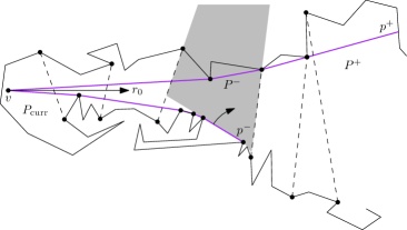
Figure 7: Procedure Catch-up: Growing the shorter side of the funnel

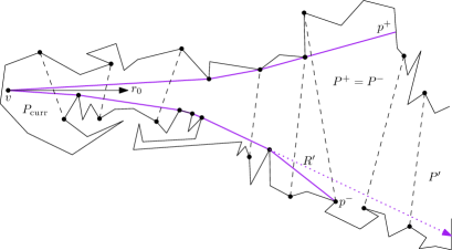
Figure 8: Procedure Extend. The ray $R^{\prime}$ splits the funnel into two funnels.

We have to implement the procedures carefully so that we do not exceed the storage bounds. Therefore, we do not store the whole funnel boundaries SP⁺ and SP^- explicitly, but we store of each SP only the first edge, the two last edges, and the $O(s)$ SP edges that cross some cut edge. We will now give the details of the two procedures.

Procedure Catch-up. We have computed the shortest path SP^- to some point $p^{-}$ in the subpolygon $P^{-}$, and our goal is to proceed towards the lower endpoint of the exit of $P^{-}$. For this, we perform a clockwise sweep of a ray whose initial point is $p^{-}$ and whose original direction follows the last edge of SP^-, until we find the first vertex of the lower boundary of $P^{-}$ that is hit, see Figure 7.

Two cases can happen depending on where the new vertex $w$ lies. If it makes a right turn with the last edge of SP^-, we have found one more edge of the funnel. Thus, we add edge $p^{-}w$ to the funnel, and continue. If $w$ makes a left turn, we must remove vertices from $P^{-}$ (so as to satisfy the invariant of the funnel). Those vertices are removed from $p^{-}$ towards $v$, and also, after reaching $v$, from the beginning of SP⁺ (in the latter case we output the removed vertices as shortest path vertices). Finally, we add a new edge to SP^-.

Since we do not explicitly store SP^- and SP⁺, when removing a SP vertex, we may have to look for the predecessor (or successor) edges by angular sweeps. Suppose $e$ is an edge of SP^- whose predecessor we want to determine. If the predecessor of $e$ crosses the entrance of the current subpolygon, we can find it in constant time (since it was explicitly stored). Otherwise, let $z$ be the initial point of $e$. We perform a counter-clockwise angular sweep of the ray with start vertex $z$ and whose initial direction is the direction of $e$, until we hit the first vertex that comes before $z$ on the lower boundary of the relevant subpolygon. This takes $O(n/s)$ time for each predecessor or successor that we need to find. The procedure for finding successor edges is symmetrical.

That is, regardless of where $v$ lies, we can a new edge to the funnel. Once this edge is found, we check where our target lies, and act using the AMRW-strategy. We can repeat this operation until we eventually find the lower end of the exit of $P^{-}$ (for example, after Catch-up has been executed in Figure 7). In this case, we advance $P^{-}$ to the next subpolygon, and we iterate until we reach the entrance of $P^{+}$.

Procedure Extend. We have now two funnel endpoints in the same subpolygon $P^{+}=P^{-}$. If both SP⁺ and SP^- have only one edge, we can switch back to the standard situation, letting the triple $(v,r_{1},r_{2})$ represent the funnel.

Thus, suppose w.l.o.g. that SP^- has more than one edge. We take the next-to-last edge $e^{\prime}$ of SP^- and shoot a ray in the direction of $e^{\prime}$ into $P^{-}$, see Figure 8. Call this ray $R^{\prime}$ and call its origin vertex $v^{\prime}$. If $R^{\prime}$ does not hit the exit of $P^{+}$, the procedure is easy: we determine, in $O(n/s)$ time, on which side of $R^{\prime}$ the target lies. If $q$ lies above $R^{\prime}$ we pop the last edge of the funnel, as in Procedure Catch-up, and proceed. If $q$ lies below $R^{\prime}$ then we report all vertices along SP^- up to $v^{\prime}$ (using the same method as in Catch-up). Then we take the triple that consists of $v^{\prime}$, the endpoint of $R^{\prime}$ and $p^{-}$, and we switch back to the standard situation (with $P_{\text{curr}}=P^{+}$).

Finally, we consider the case that $R^{\prime}$ goes through the exit, as shown in Figure 8. In this case, we extend $R^{\prime}$ until it hits the boundary of $P$, in some subpolygon $P^{\prime}$. (This takes time proportional to $n/s$ times the number of subpolygons that are traversed from $P^{+}$ to $P^{\prime}$.) Next, we determine on which side of $R^{\prime}$ the target lies. If $q$ lies above $R^{\prime}$, $R^{\prime}$ forms the new last edge of SP^-, $P^{-}$ is advanced to $P^{\prime}$, and we continue with Procedure Catch-up. If the target lies below $R^{\prime}$, we report all vertices on SP⁺ up to $v^{\prime}$, and we take a funnel that consists only of $R^{\prime}$ and the last edge of SP^-. We advance $P^{+}$ to $P^{\prime}$ and continue with Procedure Catch-up.

Runtime Analysis.

By the analysis of AMRW, in the standard situation we spend $O((n/s)^{2})$ time per subpolygon, for a total of $O(s(n/s)^{2})=O(n^{2}/s)$.

During the long-jump situation, there are $O(n)$ operations of adding or removing a vertex of the funnel: each edge is removed at most once, and even though not all vertices of the funnel are polygon vertices, it still holds that each edge of $P$ contains at most a constant number of funnel vertices.

Each funnel operation incurs an overhead of $O(n/s)$ for an angular sweep or a ray shooting operation. The only exception occurs when a ray goes through $k+1$ subpolygons, $k\geq 1$. But in this case the more advanced end of the funnel will make progress by crossing at least $k$ cut edges. Thus, the running time $O((k+1)n/s)=O(k\cdot n/s)$ for these cases cannot exceed $O(s\cdot n/s)=O(n)$ in total. We have thus obtained the following theorem.

Theorem 5.3.

Let $P$ be a simple polygon of $n$ vertices and $s$ be a parameter between $1$ and $n$. We can build a shortest-path-data structure for $P$ of size $O(s)$ in $O(n^{2})$ time and $O(s)$ work-space (or in $O(n)$ time and space). With this data structure, we can compute the shortest path within $P$ between any two points in $P$ using $O(n^{2}/s)$ time and $O(s)$ work-space. ∎

6 Open Problems

Obvious topics for future research are improvements of the results. For example, it would be interesting obtain a time-space trade-off for triangulating a PSLG. Furthermore, Theorem 5.2 describes how to find a good cut edge for a simple polygon by essentially triangulating the whole polygon and giving the most balanced cut. A natural question is if we can obtain a balanced cut in subquadratic time. The size of the smaller part should be at least a constant fraction of the whole, but it need not be $1/3$ as in Proposition 5.1. Moreover, the cut would not necessarily have to be a diagonal connecting two vertices; any straight (for example, vertical) segment partitioning the polygon would be fine.

Can the work-space for the last result on finding a shortest path between $p$ and $q$ (Theorem 5.3) be reduced to less than $O(s)$, maybe even constant? There are two components of our query algorithm that need $O(s)$ space: (i) after locating the subpolygons of $p$ and $q$ in $O(n)$ time, we identify and store the sequence of subpolygons traversed by the path, i.e., we find the path between two vertices in the tree of subpolygons. (ii) we have to process and update the funnels.

There is a chance to reduce the complexity of part (i): by the techniques of [4, Theorem 2], one can walk through the sequence of subpolygons from $p$ to $q$ in the right order in constant space and $O(s)$ time.

References

- [1] S. Arora and B. Barak. Computational Complexity – A Modern Approach. Cambridge University Press, 2009.
- [2] T. Asano, K. Buchin, M. Buchin, M. Korman, W. Mulzer, G. Rote, and A. Schulz. Memory-constrained algorithms for simple polygons. In W. Didimo and G. Liotta, editors, Abstracts of the 28th European Workshop on Computational Geometry (EuroCG’12), pages 49–52, March 2012.
- [3] T. Asano, W. Mulzer, G. Rote, and Y. Wang. Constant-work-space algorithms for geometric problems. J. Computat. Geometry, 2(1):46–68, 2011.
- [4] T. Asano, W. Mulzer, and Y. Wang. Constant-work-space algorithms for shortest paths in trees and simple polygons. Journal of Graph Algorithms and Applications, 5(5):569–586, 2011.
- [5] L. Barba, M. Korman, S. Langerman, and R. Silveira. Computing the visibility polygon using few variables. In Proc. 22nd Annu. Internat. Sympos. Algorithms Comput. (ISAAC), volume 7074 of Lecture Notes in Computer Science, pages 80–89, 2011.
- [6] M. de Berg, O. Cheong, M. van Kreveld, and M. Overmars. Computational Geometry: Algorithms and Applications. Springer-Verlag, 3rd edition, 2008.
- [7] H. Brönnimann and T. M. Chan. Space-efficient algorithms for computing the convex hull of a simple polygonal line in linear time. Comput. Geom. Theory Appl., 34(2):75–82, 2006.
- [8] H. Brönnimann, T. M. Chan, and E. Y. Chen. Towards in-place geometric algorithms and data structures. In Proc. 20th Annu. ACM Sympos. Comput. Geom. (SoCG), pages 239–246, 2004.
- [9] H. Brönnimann, J. Iacono, J. Katajainen, P. Morin, J. Morrison, and G. T. Toussaint. Space-efficient planar convex hull algorithms. Theoret. Comput. Sci., 321(1):25–40, 2004.
- [10] T. Chan and E. Chen. Multi-pass geometric algorithms. Discrete Comput. Geom., 37(1):79–102, 2007.
- [11] T. M. Chan. Comparison-based time-space lower bounds for selection. ACM Trans. Algorithms, 6(2):Art. #26, 16 pp., 2010.
- [12] T. M. Chan and E. Y. Chen. Optimal in-place and cache-oblivious algorithms for 3-d convex hulls and 2-d segment intersection. Comput. Geom. Theory Appl., 43(8):636–646, 2010.
- [13] B. Chazelle. A theorem on polygon cutting with applications. In Proc. 23rd Annu. IEEE Sympos. Found. Comput. Sci. (FOCS), pages 339–349, 1982.
- [14] B. Chazelle. Triangulating a simple polygon in linear time. Discrete Comput. Geom., 6:485–524, 1991.
- [15] B. Chazelle and J. Incerpi. Triangulation and shape-complexity. ACM Trans. Graph., 3:135–152, 1984.
- [16] H. ElGindy, H. Everett, and G. Toussaint. Slicing an ear using prune-and-search. Pattern Recogn. Lett., 14(9):719–722, 1993.
- [17] A. Fournier and D. Y. Montuno. Triangulating simple polygons and equivalent problems. ACM Trans. Graph., 3:153–174, 1984.
- [18] G. N. Frederickson. Upper bounds for time-space trade-offs in sorting and selection. J. Comput. System Sci., 34(1):19–26, 1987.
- [19] M. R. Garey, D. S. Johnson, F. P. Preparata, and R. E. Tarjan. Triangulating a simple polygon. Inform. Process. Lett., 7(4):175–179, 1978.
- [20] L. J. Guibas and J. Hershberger. Optimal shortest path queries in a simple polygon. J. Comput. System Sci., 39(2):126–152, 1989.
- [21] G. Jacobson. Succinct Static Data Structures. PhD thesis, Carnegie-Mellon, January 1989. Tech Rep CMU-CS-89-112.
- [22] J. Munro and M. Paterson. Selection and sorting with limited storage. Theoret. Comput. Sci., 12:315–323, 1980.
- [23] J. I. Munro and V. Raman. Selection from read-only memory and sorting with minimum data movement. Theoret. Comput. Sci., 165(2):311–323, 1996.
- [24] S. Muthukrishnan. Data streams: algorithms and applications. Found. Trends Theor. Comput. Sci., 1(2):117–236, 2005.
- [25] V. Raman and S. Ramnath. Improved upper bounds for time-space tradeoffs for selection with limited storage. In Proc. 6th Scandinavian Workshop on Algorithm Theory (SWAT), volume 1432 of Lecture Notes in Computer Science, pages 131–142, 1998.
- [26] O. Reingold. Undirected connectivity in log-space. J. ACM, 55(4):Art. #17, 24 pp., 2008.
- [27] R. Seidel. Convex hull computations. In Handbook of Discrete and Computational Geometry, chapter 22, pages 495–512. CRC Press, Inc., 2nd edition, 2004.