Postprocessing and Higher Order Convergence of Stabilized Finite Element Discretizations of the Stokes Eigenvalue Problem

Abstract

In this paper, the stabilized finite element method based on local projection is applied to discretize the Stokes eigenvalue problems and the corresponding convergence analysis is given. Furthermore, we also use a method to improve the convergence rate for the eigenpair approximations of the Stokes eigenvalue problem. It is based on a postprocessing strategy that contains solving an additional Stokes source problem on an augmented finite element space which can be constructed either by refining the mesh or by using the same mesh but increasing the order of mixed finite element space. Numerical examples are given to confirm the theoretical analysis.

Keywords. Stokes eigenvalue problem, finite element method, local projection stabilization, Rayleigh quotient formula, postprocessing, two-grid, two spaces

AMS subject classifications. 65N30, 65N25, 65L15, 65B99

1 Introduction

In this paper, we are concerned with the Stokes eigenvalue problems. The study of Stokes eigenmodes is required when the dynamics behaviors governed by the Navier-Stokes equations result from the way this nonlinear dynamics is controlled by diffusion. For the other reasons to study the Stokes eigenmodes, please read the papers [6, 22].

The Stokes eigenvalue problem reads as follows:

Find $({\mathbf{u}},p,\lambda)$ such that

$$\left\{\begin{array}[]{rcl}-\Delta{\mathbf{u}}+\nabla p&=&\lambda{\mathbf{u}}\ \ \ {\rm in}\ \Omega,\\ \nabla\cdot{\mathbf{u}}&=&0\ \ \ \ \ {\rm in}\ \Omega,\\ {\mathbf{u}}&=&0\ \ \ \ \ {\rm on}\ \partial\Omega,\\ \int_{\Omega}{\mathbf{u}}^{2}d\Omega&=&1,\end{array}\right.$$ (1.1)

where $\Omega\subset\mathbb{R}^{2}$ is a bounded domain with Lipschitz boundary $\partial\Omega$ and $\Delta$, $\nabla$, $\nabla\cdot$ denote the Laplacian, gradient and divergence operators, respectively.

There are several works for the eigenvalue problems and their numerical methods such as Babuška and Osborn [2, 3, 29], Mercier, Osborn, Rappaz and Raviart [27], etc. Osborn [29], Mercier, Osborn, Rappaz and Raviart [27] give an abstract analysis for the eigenpair approximations by mixed/hybrid finite element methods based on the general theory of compact operators ([13]). In [21] and [24], a posteriori error estimates and the corresponding adaptive finite element methods are given for the Stokes eigenvalue problems.

The first aim in this paper is to use the local projection stabilization method to discretize the Stokes eigenvalue problems. The local projection stabilization (LPS) method has been proposed for the Stokes problem in [7]. The extension to the transport problem was given in [8]. The analysis of the local projection method applied to equal-order interpolation discretization can be found [25] for Oseen problem and in [26] for convection-diffusion problem.

The stabilization term of the local projection method is based on a projection $\pi_{h}:V_{h}\to\mathcal{D}_{h}$ of the finite element space $V_{h}$ which approximates the solution into a discontinuous space $\mathcal{D}_{h}$. The standard Galerkin discretization is stabilized by adding a term which gives $L^{2}$ control over the fluctuation $id-\pi_{h}$ of the gradient of the solution. Here, the LPS method is based on the approximation space $V_{h}$ and the projection space $\mathcal{D}_{h}$ are defined on the same mesh. In this case, the approximation space $V_{h}$ is enriched to satisfy the local inf-sup condition guaranteeing the existence of an interpolation with an orthogonal property compared to standard finite element spaces. For more details, please read the book [31].

Recently, many effective postprocessing methods that improve the convergence rate for the approximations of the eigenvalue problems by the finite element methods have been proposed and analyzed ([1, 30, 35]). Xu and Zhou [35] have given a two-grid discretization technique to improve the convergence rate of the second order elliptic eigenvalue problems and integral eigenvalue problems. Racheva and Andreev [30], Andreev, Lazarov and Racheva [1] have proposed a postprocessing method that improve the convergence rate for the numerical approximations of $2m$-order selfadjoint eigenvalue problems especially biharmonic eigenvalue problems. In [15], a similar method has been given for the Stokes eigenvalue problem by mixed finite element methods. The second aim of this paper is to propose and analyze a postprocessing algorithm which can improve the convergence rate of the eigenpair approximations for the Stokes eigenvalue problem by the LPS method.

The postprocessing procedure can be described as follows: (1) solve the Stokes eigenvalue problem in the original finite element space; (2) solve an additional Stokes source problem in an augmented space using the previous obtained eigenvalue multiplying the corresponding eigenfunction as the load vector. This method can improve the convergence rate of the eigenpair approximations with relative inexpensive computation because we replace the solution of the eigenvalue problem by an additional source problem on a finer mesh or in a higher order finite element space.

An outline of the paper goes as follows. In Section 2, we introduce the application of LPS method for Stokes eigenvalue problem. The corresponding error estimate is given in section 3. Section 4 is devoted to deriving the postprocessing technique and analyze its efficiency. In Section 5, we propose a practical computational algorithm to implement the postprocessing method. In Section 6, we give two numerical results to confirm the theoretical analysis. Some concluding remarks are given in the last section.

2 Discretizations of the Stokes eigenvalue problem

In this paper, we use the standard notations ([11, 12, 16]) for the Sobolev spaces $H^{m}(\Omega)$ (standard interpolation spaces for real number $m$) and their associated inner products $(\cdot,\cdot)_{m}$, norms $\|\cdot\|_{m}$ and seminorms $|\cdot|_{m}$ for $m\geq 0$. The Sobolev space $H^{0}(\Omega)$ coincides with $L^{2}(\Omega)$, in which case the norm and inner product are denoted by $\|\cdot\|$ and $(\cdot,\cdot)$, respectively. In addition, denoted by $L^{2}_{0}(\Omega)$ the subspace of $L^{2}(\Omega)$ that consists of functions on $L^{2}(\Omega)$ having mean value zero. We also use the vector valued functions $(H^{m}(\Omega))^{2}$ just as [12] and [20].

The corresponding weak form of (1.1) is:

Find $({\bf u},p,\lambda)\in{\bf V}\times Q\times\mathbb{R}$ such that $r({\mathbf{u}},{\mathbf{u}})=1$ and

$$\left\{\begin{array}[]{rcl}a({\mathbf{u}},{\mathbf{v}})-b({\mathbf{v}},p)&=&\lambda r({\mathbf{u}},{\mathbf{v}})\ \ \ \forall{\mathbf{v}}\in{\bf V},\\ b({\mathbf{u}},q)&=&0\ \ \ \ \ \ \ \ \ \ \ \ \forall q\in Q,\end{array}\right.$$ (2.1)

where ${\bf V}=(H_{0}^{1}(\Omega))^{2}$, $Q=L_{0}^{2}(\Omega)$ and

$$a({\mathbf{u}},{\mathbf{v}}) = \int_{\Omega}\nabla{\mathbf{u}}\nabla{\bf v}d\Omega,$$

$$b({\mathbf{v}},p) = \int_{\Omega}\nabla\cdot{\mathbf{v}}pd\Omega,$$

$$r({\mathbf{u}},{\mathbf{v}}) = \int_{\Omega}{\mathbf{u}}{\bf v}d\Omega.$$

From [3], we know eigenvalue problem (2.1) has an eigenvalue sequence $\{\lambda_{j}\}$:

$$0<\lambda_{1}\leq\lambda_{2}\leq\cdots\leq\lambda_{k}\leq\cdots,\ \ \lim_{k\rightarrow\infty}\lambda_{k}=\infty,$$

and the associated eigenfunctions

$$({\mathbf{u}}_{1},p_{1}),({\mathbf{u}}_{2},p_{2}),\cdots,({\mathbf{u}}_{k},p_{k}),\cdots,$$

where $r({\mathbf{u}}_{i},{\mathbf{u}}_{j})=\delta_{ij}$.

For the aim of analysis, we define the bilinear form as

$$A((\mathbf{u},p);(\mathbf{v},q)) = a(\mathbf{u},\mathbf{v})-b(\mathbf{v},p)+b(\mathbf{u},q).$$ (2.2)

For simplicity, we only consider the simple eigenvalues in this paper. We know that $a(\cdot,\cdot),b(\cdot,\cdot)$ and $s(\cdot,\cdot)$ have the following properties ([20]):

$$a({\mathbf{u}},{\mathbf{v}}) \leq\|\mathbf{u}\|_{1}\|\mathbf{v}\|_{1},$$ (2.3)

$$a({\mathbf{u}},{\mathbf{u}}) \geq C\|\mathbf{u}\|_{1}^{2},$$ (2.4)

$$r({\mathbf{u}},{\mathbf{v}}) \leq C\|{\mathbf{u}}\|_{0}\|{\mathbf{v}}\|_{0},$$ (2.5)

$$r({\mathbf{u}},{\mathbf{u}}) \geq C\|{\mathbf{u}}\|_{0}^{2},$$ (2.6)

$$\sup_{0\neq{\bf v}\in{\bf V}}\frac{b({\mathbf{v}},q)}{\|{\bf v}\|_{1}} \geq C\|q\|_{0},$$ (2.7)

$$\|{\mathbf{u}}\|_{1}+\|p\|_{0} \leq C\sup_{0\neq({\mathbf{v}},q)\in{\bf V}\times Q}\frac{A((\mathbf{u},p);(\mathbf{v},q))}{\|{\mathbf{v}}\|_{1}+\|q\|_{0}},$$ (2.8)

where $C>0$. In this paper, $C$ denotes constant independent of the mesh size $h$ and sometimes depends on the eigenvalue $\lambda$ and may be different values at its different occurrence.

For the eigenvalue, there exists the following Rayleigh quotient expression

$$\lambda=\frac{a({\mathbf{u}},{\mathbf{u}})}{r({\mathbf{u}},{\bf u})}.$$ (2.9)

2.1 Local projection stabilization

In this section, we consider equal order interpolations stabilized by the local projection method in its one-level variant as developed in [19, 25]. For the two-level approach we refer to [7, 10, 28]. Let $V_{h}$ denote a scalar finite element space of continuous, piecewise polynomials over $\mathcal{T}_{h}$. The spaces for approximating velocity and pressure are given by $\mathbf{V}_{h}:=V_{h}^{2}\cap\mathbf{V}$ and $Q_{h}:=V_{h}\cap Q$. The discrete problem of our stabilized method is:

Find $(\mathbf{u}_{h},p_{h})\in\mathbf{V}_{h}\times Q_{h}$ such that

$$\left\{\begin{array}[]{rcl}a({\mathbf{u}}_{h},{\mathbf{v}})-b({\mathbf{v}},p_{h})&=&\lambda_{h}r({\mathbf{u}}_{h},{\mathbf{v}})\ \ \ \ \forall{\bf v}\in{\bf V}_{h},\\ b({\mathbf{u}}_{h},q)+S_{h}(p_{h},q_{h})&=&0\ \ \ \ \ \ \ \ \ \quad\quad\ \forall q\in Q_{h},\end{array}\right.$$ (2.10)

where the stabilization term with user-chosen parameters $\alpha_{K}$ is given by

$$S_{h}(p,q)=\sum_{K\in\mathcal{T}_{h}}\alpha_{K}(\kappa_{h}\nabla p,\kappa_{h}\nabla q)_{K}.$$ (2.11)

Here, the fluctuation operator $\kappa_{h}:L^{2}(\Omega)\rightarrow L^{2}(\Omega)$ acting componentwise is defined as follows. Let $P_{s}(K)$ denote the set of all polynomials of degree less than or equal to $s$ and let $D_{h}(K)$ be a finite dimensional space on the cell $K\in{\mathcal{T}}_{h}$ with $P_{s}(K)\subset D_{h}(K)$. We extend the definition by allowing $P_{-1}(K)=D_{h}(K)=\{0\}$. We introduce the associated global space of discontinuous finite elements

$$D_{h}:=\bigoplus_{K\in{\mathcal{T}}_{h}}D_{h}(K)$$

and the local $L^{2}(K)$-projection $\pi_{K}:L^{2}(K)\rightarrow D_{h}(K)$ generating the global projection $\pi_{h}:L^{2}(\Omega)\rightarrow D_{h}$ by

$$(\pi_{h}w)\big{|}_{K}:=\pi_{K}(w|_{K})\qquad\forall K\in{\mathcal{T}}_{h},\;\forall w\in L^{2}(\Omega).$$

The fluctuation operator $\kappa_{h}:L^{2}(\Omega)\rightarrow L^{2}(\Omega)$ used in (2.11) is given by $\kappa_{h}:=id-\pi_{h}$ where $id:L^{2}(\Omega)\rightarrow L^{2}(\Omega)$ is the identity on $L^{2}(\Omega)$.

In order to study the convergence properties of this method for Stokes eigenvalue problem, we introduce the bilinear form

$$A_{h}((\mathbf{u},p);(\mathbf{v},q)) =(\nabla\mathbf{u},\nabla\mathbf{v})-(p,\text{div }\mathbf{v})+(q,\text{div }\mathbf{u})+S_{h}(p,q).$$ (2.12)

and the mesh-dependent norm

$$|||(\mathbf{v},q)|||_{A} :=\Bigl{(}|\mathbf{v}|_{1}^{2}+\|q\|_{0}^{2}+\sum_{K\in\mathcal{T}_{h}}\alpha_{K}\|\kappa_{h}\nabla q\|_{0,K}^{2}\Bigr{)}^{1/2}.$$ (2.13)

The existence and uniqueness of discrete solutions of Stokes problem have been studied in [25, 19] for different pairs $(V_{h},D_{h})$ of approximation and projection spaces, respectively. Based on these results, the existence and uniqueness of eigenvalue problem (2.10) can be given similarly.

The stability and convergence properties of the LPS method (2.10) need the following assumptions([25, 31]).
Assumption A1: There is an interpolation operator $i_{h}:H^{2}(\Omega)\to V_{h}$ such that

$$\|v-i_{h}v\|_{0,K}+h_{K}|v-i_{h}v|_{1,K}\leq Ch_{k}^{l}\|v\|_{l,\omega(K)}\ \$$ (2.14)

for all $K\in\mathcal{T}_{h}$, $v\in H^{l}(\omega(K))$ and $1\leq l\leq k+1$, where $\omega(K)$ denotes a certain local neighborhood of $K$ which appears in the definition of these interpolation operators for non-smooth functions; see [17, 33] for more details.
Assumption A2: The fluctuation operator $\kappa_{h}$ satisfy the following approximation property

$$\|\kappa_{h}q\|_{0,K}\leq Ch^{l}_{K}|q|_{l,K}\ \ \ \forall K\in\mathcal{T}_{h},\>\forall q\in H^{l}(K),\>0\leq l\leq k.$$ (2.15)

Assumption A3: There exists a constant $\beta_{1}>0$ such that for all $h>0$

$$\inf_{{q_{h}\in\mathcal{D}_{h}(K)}}\sup_{{v_{h}\in V_{h}(K)}}\frac{(v_{h},q_{h})}{\|v_{h}\|_{0,K}\>\|q_{h}\|_{0,K}}\geq\beta_{1}>0$$ (2.16)

is satisfied where $V_{h}(K)=\{v_{h}|_{K}:v_{h}\in V_{h},\ v_{h}=0\ {\rm in}\ \Omega\backslash K\}$.

The assumption A1 and A3 guarantee the existence of an interpolant with the usual interpolation properties (2.14) and the orthogonality

$$(v-j_{h}v,q_{h})=0\ \ \ \ \forall q_{h}\in\mathcal{D}_{h},\forall v\in H^{2}(\Omega),$$ (2.17)

whereas A2 is needed to bound the consistency error [31]. For example, in the one-level LPS assumption A1 and A2 are satisfied if we choose $(V_{h},D_{h})=(P_{k},P_{k-1}^{\rm disc})$ continuous and discontinuous, piecewise polynomials of degree $r$ and $r-1$, respectively. In order to guarantee A3, $V_{h}$ need to be enriched by suitable bubble functions. For more details about LPS method, please read the papers [25, 26] and the book [31].

Lemma 2.1.

([19]) Let the assumption A1, A3, and $\alpha_{K}\sim h_{K}^{2}$ be fulfilled. Then, there is a positive constant $\beta_{A}$ independent of $h$ such that

$$\inf_{(\mathbf{v}_{h},q_{h})\in\mathbf{V}_{h}\times Q_{h}}\sup_{(\mathbf{w}_{h},r_{h})\in\mathbf{V}_{h}\times Q_{h}}\frac{A_{h}\big{(}(\mathbf{v}_{h},q_{h});(\mathbf{w}_{h},r_{h})\big{)}}{|||(\mathbf{v}_{h},q_{h})|||_{A}\;|||(\mathbf{w}_{h},r_{h})|||_{A}}\geq\beta_{A}>0$$ (2.18)

holds.

Based on Lemma 2.1, the discrete Stokes eigenvalue problem (2.10) is consistent with the continuous problem (2.1) ([19]).

3 Convergence analysis

In thois section, we give the convergence analysis for the eigenpair approximation $(\mathbf{u}_{h},p_{h},\lambda_{h})$ in (2.10).

We know that the convergence rate of the eigenpair approximations by the finite element methods depends on the regularities of the exact eigenfunctions. The exact eigenfunctions of the Stokes problem only belong to the space $(H^{1}(\Omega))^{2}\times H^{0}(\Omega)$ on general domains. But for the domains with smooth boundary, the exact eigenfunctions have additional regularities. In this case we need to use isoparametric mixed finite element methods to fit the domain more exactly ([11] and [16]). The goals of this paper are to use LPS method to solve the Stokes eigenvalue problem, and propose and analyze a postprocessing method which can improve the convergence rate for both eigenvalue and eigenfunction approximations. The assumption that $\Omega$ is a convex polygonal domain can make the expression of the main idea of this paper more directly. But, we need to notice that this assumption limits the regularity of the exact eigenfunctions and makes the analysis of the convergence rates much more complicated. It is well known ([4, 5, 18]) that for a given ${\bf f}\in(H^{\gamma}(\Omega))^{2}$ the solution $({\mathbf{u}},p)$ of the corresponding Stokes problem

$$\left\{\begin{array}[]{rcl}a({\mathbf{u}},{\mathbf{v}})-b({\bf v},p)&=&r({\bf f},{\mathbf{v}})\ \ \ \forall{\mathbf{v}}\in{\bf V},\\ b({\mathbf{u}},q)&=&0\ \ \quad\quad\forall q\in Q\end{array}\right.$$ (3.1)

has the following regularity ([4, 5, 9, 18])

$$\|{\mathbf{u}}\|_{2+\gamma}+\|p\|_{1+\gamma}\leq C\|{\bf f}\|_{\gamma}\ \ \ \forall{\bf f}\in(H^{\gamma}(\Omega))^{2},$$ (3.2)

where $0<\gamma\leq 1$ is a parameter that depends on the largest interior angle of $\partial\Omega$ ([4]).

From (2.10), we can know the following Rayleigh quotient for $\lambda_{h}$ holds

$$\lambda_{h}=\frac{a({\mathbf{u}}_{h},{\mathbf{u}}_{h})}{r({\mathbf{u}}_{h},{\mathbf{u}}_{h})}$$ (3.3)

Holds.

It is also known from [3] the Stokes eigenvalue problem (2.10) has eigenvalues

$$0<(\lambda_{1})_{h}\leq(\lambda_{2})_{h}\leq\cdots\leq(\lambda_{k})_{h}\leq\cdots\leq(\lambda_{N})_{h},$$

and the corresponding eigenfunctions

$$(({\mathbf{u}}_{1})_{h},(p_{1})_{h}),(({\mathbf{u}}_{2})_{h},(p_{2})_{h}),\cdots,(({\mathbf{u}}_{k})_{h},(p_{k})_{h}),\cdots,(({\mathbf{u}}_{N})_{h},(p_{N})_{h}),$$

where $r(({\mathbf{u}}_{i})_{h},({\bf u}_{j})_{h})=\delta_{ij},1\leq i,j\leq N$, $N$ denotes the dimension of the finite element space $\mathbf{V}_{h}\times Q_{h}$ .

Let us define the compact operator $T:(L^{2}(\Omega))^{2}\rightarrow(H^{1}(\Omega))^{2}$ and the operator $K:(L^{2}(\Omega))^{2}\rightarrow L^{2}_{0}(\Omega)$ by

$$A((T\mathbf{f},K\mathbf{f}),(\mathbf{v},q)) = r(\mathbf{f},\mathbf{v}),\ \ \ \forall(\mathbf{v},q)\in(H_{0}^{1}(\Omega))^{2}\times L_{0}^{2}(\Omega).$$ (3.4)

Hence the eigenvalue problem (2.1) can be written as

$$\lambda T\mathbf{u} = \mathbf{u}.$$ (3.5)

Let $M(\lambda_{i})$ denote the eigenspace corresponding to the eigenvalue $\lambda_{i}$ which is defined by

$$M(\lambda_{i}) = \Big{\{}(\mathbf{w},\psi)\in(H_{0}^{1}(\Omega))^{2}\times L_{0}^{2}(\Omega):\ (\mathbf{w},\psi)\ {\rm is\ an\ eigenfunction\ of}\ (\ref{wstokesproblem})$$

$$\ \ \ \ \ {\rm corresponding\ to\ }\lambda_{i}\ {\rm and}\ r(\mathbf{w},\mathbf{w})=1\Big{\}}.$$

Similarly, we also introduce the discrete operator $T_{h}:(L^{2}(\Omega))^{2}\rightarrow\mathbf{V}_{h}$ and the operator $K_{h}:(L^{2}(\Omega))^{2}\rightarrow Q_{h}$ by

$$A_{h}((T_{h}\mathbf{f},K_{h}\mathbf{f}),(\mathbf{v},q)) = r(\mathbf{f},\mathbf{v}),\ \ \ \forall(\mathbf{v},\mathbf{q})\in\mathbf{V}_{h}\times Q_{h}.$$ (3.6)

Hence the operator form of the discrete eigenvalue problem (2.10) is

$$\lambda_{h}T_{h}\mathbf{u}_{h} = \mathbf{u}_{h}.$$ (3.7)

In [19], the convergence result of LPS method for Stokes problems has been given. Combining abstract spectral approximation results from [3], we can give the convergence results for the Stokes eigenvalue problem by LPS method. The eigenvalue approximation $\lambda_{h}$ and the corresponding eigenfunction approximation $({\mathbf{u}}_{h},p_{h})$ have the following error bounds ([2, 29, 18, 19, 27, 20]):

$$\|\mathbf{u}-\mathbf{u}_{h}\|_{1} \leq C\|(T-T_{h})|_{M(\lambda)}\|_{1}.$$ (3.8)

In order to do the analysis for the postprocessing in the following sections, we also need the convergence result for the eigenfunction approximation $\mathbf{u}_{h}$ in $H^{-1}$-norm. For this aim, based on the result in [2], we first need to use the duality argument to get $H^{-1}$-norm error estimate for the finite element projection and the process is similar to the one in the paper [19] for the $L^{2}$-norm error estimate.

The finite element projection $(R_{h}\mathbf{u},R_{h}p)$ denotes the finite element solution of the following Stokes problem:

Find $(R_{h}(\mathbf{u},p),G_{h}(\mathbf{u},p))\in\mathbf{V}_{h}\times Q_{h}$ such that

$$A_{h}((R_{h}(\mathbf{u},p),G_{h}(\mathbf{u},p));(\mathbf{v},q))=A((\mathbf{u},p);(\mathbf{v},q))\ \ \ \forall(\mathbf{v},q)\in\mathbf{V}_{h}\times Q_{h}.$$ (3.9)

$$T_{h}=R_{h}(T,K), K_{h}=G_{h}(T,K).$$ (3.10)

$$\|\mathbf{u}-\mathbf{u}_{h}\|_{1} \leq C\|(T-R_{h}(T,K)|_{M(\lambda)}\|_{1}.$$ (3.11)

From the definition, we have the orthogonal relation

$$A_{h}((\mathbf{u}-R_{h}(\mathbf{u},p),p-G_{h}(\mathbf{u},p));(\mathbf{v},q)) = S_{h}(p,q)$$ (3.12)

$$\ \ \forall(\mathbf{v},q)\in\mathbf{V}_{h}\times Q_{h}.$$

$$|||(\mathbf{v}_{h}-R_{h}(\mathbf{u},p),q_{h}-G_{h}(\mathbf{u},p))|||_{A}$$ (3.13)

$$\leq \frac{1}{\beta_{A}}\sup_{0\neq(\mathbf{w}_{h},\psi_{h})\in\mathbf{V}_{h}\times Q_{h}}\frac{A_{h}((\mathbf{v}_{h}-R_{h}(\mathbf{u},p),q_{h}-G_{h}(\mathbf{u},p));(\mathbf{w}_{h},\psi_{h}))}{|||(\mathbf{w}_{h},\psi_{h})|||_{A}}$$

$$\leq \frac{1}{\beta_{A}}\sup_{0\neq(\mathbf{w}_{h},\psi_{h})\in\mathbf{V}_{h}\times Q_{h}}\frac{A_{h}((\mathbf{v}_{h}-\mathbf{u},q_{h}-p);(\mathbf{w}_{h},\psi_{h}))}{|||(\mathbf{w}_{h},\psi_{h})|||_{A}}$$

$$+\frac{1}{\beta_{A}}\sup_{0\neq(\mathbf{w}_{h},\psi_{h})\in\mathbf{V}_{h}\times Q_{h}}\frac{A_{h}((\mathbf{u}-R_{h}(\mathbf{u},p),p-G_{h}(\mathbf{u},p));(\mathbf{w}_{h},\psi_{h}))}{|||(\mathbf{w}_{h},\psi_{h})|||_{A}}$$

$$\leq \frac{C}{\beta_{A}}|||(\mathbf{u}-\mathbf{v}_{h},p-q_{h})|||_{A}+\frac{1}{\beta_{A}}\sup_{0\neq(\mathbf{w}_{h},\psi_{h})\in\mathbf{V}_{h}\times Q_{h}}\frac{S_{h}(p,\psi_{h})}{|||(\mathbf{w}_{h},\psi_{h})|||_{A}}$$

$$\leq \frac{C}{\beta_{A}}|||(\mathbf{u}-\mathbf{v}_{h},p-q_{h})|||_{A}+\frac{1}{\beta_{A}}S_{h}^{1/2}(p,p)$$

$$|||(\mathbf{u}-R_{h}(\mathbf{u},p),p-G_{h}(\mathbf{u},p))|||_{A}$$ (3.14)

$$\leq |||(\mathbf{u}-\mathbf{v}_{h},p-q_{h})|||_{A}+|||(\mathbf{v}_{h}-R_{h}(\mathbf{u},p),q_{h}-G_{h}(\mathbf{u},p))|||_{A}$$

$$\leq C|||(\mathbf{u}-\mathbf{v}_{h},p-q_{h})|||_{A}+CS_{h}^{1/2}(p,p).$$

The arbitrariness of $(\mathbf{v}_{h},q_{h})$ leads to the following

$$|||(\mathbf{u}-R_{h}(\mathbf{u},p),p-G_{h}(\mathbf{u},p))|||_{A}$$ (3.15)

$$\leq C\big{(}\inf_{(\mathbf{v}_{h},q_{h})\in\mathbf{V}_{h}\times Q_{h}}|||(\mathbf{u}-\mathbf{v}_{h},p-q_{h})|||_{A}+S_{h}^{1/2}(p,p)\big{)}.$$

$$\|\mathbf{u}-\mathbf{u}_{h}\|_{1} \leq C\delta_{h}(\lambda),$$ (3.16)

where $\delta_{h}(\lambda)$ is defined by

$$\delta_{h}(\lambda):=\sup_{(\mathbf{w},\psi)\in M(\lambda)}\big{(}\inf_{(\mathbf{v}_{h},q_{h})\in\mathbf{V}_{h}\times Q_{h}}|||(\mathbf{w}-\mathbf{v}_{h},\psi-q_{h})|||_{A}+S_{h}^{1/2}(\psi,\psi)\big{)}.$$ (3.17)

We choose $\mathbf{g}\in(H_{0}^{1}(\Omega))^{2}$ such that $\|\mathbf{g}\|_{1}=1$ and

$$\|\mathbf{u}-R_{h}(\mathbf{u},p)\|_{-1} = r(\mathbf{u}-R_{h}(\mathbf{u},p),\mathbf{g}).$$

Then we define a duality problem corresponding to $\mathbf{g}$:

Find $(\mathbf{u}_{g},p_{g})\in\mathbf{V}\times Q$ such that

$$\left\{\begin{array}[]{rcl}a(\mathbf{v},\mathbf{u}_{g})-b(\mathbf{v},p_{g})&=&r(\mathbf{v},\mathbf{g})\ \ \ \ \forall\mathbf{v}\in\mathbf{V},\\ b(\mathbf{u}_{g},q)&=&0\quad\quad\quad\ \ \forall q\in Q.\end{array}\right.$$ (3.18)

Combination of (3.12) and (3.18) derives the following estimate

$$r(\mathbf{u}-R_{h}(\mathbf{u},p),\mathbf{g}) = a(\mathbf{u}-R_{h}(\mathbf{u},p),\mathbf{u}_{g})-b(\mathbf{u}-R_{h}(\mathbf{u},p),p_{g})$$

$$= a(\mathbf{u}-R_{h}(\mathbf{u},p),\mathbf{u}_{g}-\mathbf{v}_{h})-b(\mathbf{u}-R_{h}(\mathbf{u},p),p_{g}-q_{h})$$

$$-b(\mathbf{u}_{g}-\mathbf{v}_{h},p-G_{h}(\mathbf{u},p))-S_{h}(G_{h}(\mathbf{u},p),q_{h})$$

$$= a(\mathbf{u}-R_{h}(\mathbf{u},p),\mathbf{u}_{g}-\mathbf{v}_{h})-b(\mathbf{u}-R_{h}(\mathbf{u},p),p_{g}-q_{h})$$

$$-b(\mathbf{u}_{g}-\mathbf{v}_{h},p-G_{h}(\mathbf{u},p))-S_{h}(p-G_{h}(\mathbf{u},p),p_{g}-q_{h})$$

$$+S_{h}(p-G_{h}(\mathbf{u},p),p_{g})+S_{h}(p,p_{g}-q_{h})-S_{h}(p,p_{g}).$$

Choosing $(\mathbf{v}_{h},q_{h})\in\mathbf{V}_{h}\times Q_{h}$ as an interpolant of $(\mathbf{u}_{g},p_{g})$, we obtain

$$|r(\mathbf{u}-R_{h}(\mathbf{u},p),\mathbf{g})|$$

$$\leq C\big{(}\|\mathbf{u}-R_{h}(\mathbf{u},p)\|_{1}+\|p-G_{h}(\mathbf{u},p)\|_{0})(\|\mathbf{u}_{g}-\mathbf{v}_{h}\|_{1}+\|p_{g}-q_{h}\|_{0}\big{)}$$

$$+|S_{h}(G_{h}(\mathbf{u},p),q_{h})|$$

$$\leq C\big{(}|||(\mathbf{u}-R_{h}(\mathbf{u},p),p-G_{h}(\mathbf{u},p))|||_{A}+S_{h}^{1/2}(p,p)\big{)}$$

$$\ \ \ \ \big{(}|||(\mathbf{u}_{g}-\mathbf{v}_{h},p_{g}-q_{h})|||_{A}+S_{h}^{1/2}(p_{g},p_{g})\big{)}.$$

In particular, when $\Omega$ is smooth, we have the regularity estimate

$$\|\mathbf{u}_{g}\|_{3}+\|p_{g}\|_{2}\leq C\|\mathbf{g}\|_{1},$$

$$\|\mathbf{u}-R_{h}\mathbf{u}\|_{-1} \leq C\eta_{h}\delta_{h},$$

where

$$\eta_{h}=\sup_{\|\mathbf{g}\|_{1}=1}\inf_{(\mathbf{v},q)\in\mathbf{V}_{h}\times Q_{h}}\big{(}|||(T\mathbf{g}-\mathbf{v},K\mathbf{g}-q)|||_{A}+S_{h}^{1/2}(K\mathbf{g},K\mathbf{g})\big{)}.$$ (3.19)

4 One correction step

In this section, we present a type of correction step to improve the accuracy of the current eigenvalue and eigenfunction approximations. This correction method contains solving an auxiliary source problem in the finer finite element space and an eigenvalue problem on the coarsest finite element space. For simplicity of notation, we set $(\lambda,u)=(\lambda_{i},u_{i})\ (i=1,2,\cdots,k,\cdots)$ and $(\lambda_{h},u_{h})=(\lambda_{i,h},u_{i,h})\ (i=1,2,\cdots,N_{h})$ to denote an eigenpair of problem (LABEL:weak_problem) and (LABEL:weak_problem_Discrete), respectively.

To derive our method, we need first to introduce the error expansions of the eigenvalues by the Rayleigh quotient formula. It is well known that there have been the Rayleigh quotient error expansions for the eigenvalues of the second order elliptic problems ([23]).

Theorem 4.1.

Assume $({\mathbf{u}},p,\lambda)$ is the true solution of the Stokes eigenvalue problem (2.1), $0\neq{\mathbf{w}}\in(H_{0}^{1}(\Omega))^{2}$ and $\psi\in L_{0}^{2}(\Omega)$ satisfy

$$b({\mathbf{w}},\psi)+S_{h}(\psi,\psi)=0.$$ (4.1)

Let us define

$$\hat{\lambda}=\frac{a({\mathbf{w}},{\mathbf{w}})}{r({\mathbf{w}},{\bf w})}.$$ (4.2)

Then, we have

$$\hat{\lambda}-\lambda =\frac{a({\mathbf{w}}-{\mathbf{u}},{\mathbf{w}}-{\bf u})+2b({\mathbf{w}}-{\mathbf{u}},p-\psi)-\lambda r({\bf w}-{\mathbf{u}},{\mathbf{w}}-{\mathbf{u}})}{r({\mathbf{w}},{\mathbf{w}})}$$

$$\quad\quad\quad-\frac{2S_{h}(\psi,\psi)}{r({\mathbf{w}},{\mathbf{w}})}.$$ (4.3)

If the condition (4.1) is changed to be

$$b(\mathbf{w},\varphi) =0,$$ (4.4)

the expansion for $\hat{\lambda}-\lambda$ should be

$$\hat{\lambda}-\lambda =\frac{a({\mathbf{w}}-{\mathbf{u}},{\mathbf{w}}-{\bf u})+2b({\mathbf{w}}-{\mathbf{u}},p-\psi)-\lambda r({\bf w}-{\mathbf{u}},{\mathbf{w}}-{\mathbf{u}})}{r({\mathbf{w}},{\mathbf{w}})}.$$ (4.5)

Proof.

From (2.1), (2.10), (3.3), (4.1), (4.2) and direct computation, we have

$$\hat{\lambda}-\lambda = \frac{a({\mathbf{w}},{\mathbf{w}})-\lambda r({\bf w},{\mathbf{w}})}{r({\mathbf{w}},{\mathbf{w}})}$$

$$= \frac{a({\mathbf{w}}-{\mathbf{u}},{\mathbf{w}}-{\mathbf{u}})+2a({\bf w},{\bf u})-a({\mathbf{u}},{\mathbf{u}})-\lambda r({\mathbf{w}},{\bf w})}{r({\mathbf{w}},{\bf w})}$$

$$= \frac{a({\mathbf{w}}-{\mathbf{u}},{\mathbf{w}}-{\mathbf{u}})+2\lambda r({\mathbf{w}},{\mathbf{u}})+2b({\mathbf{w}},p)-\lambda r({\mathbf{u}},{\bf u})-\lambda r({\mathbf{w}},{\bf w})}{r({\mathbf{w}},{\mathbf{w}})}$$

$$= \frac{a({\mathbf{w}}-{\mathbf{u}},{\mathbf{w}}-{\mathbf{u}})-\lambda r({\mathbf{w}}-{\bf u},{\mathbf{w}}-{\mathbf{u}})+2b({\mathbf{w}},p)}{r({\mathbf{w}},{\mathbf{w}})}$$

$$= \frac{a({\mathbf{w}}-{\mathbf{u}},{\mathbf{w}}-{\mathbf{u}})-\lambda r({\mathbf{w}}-{\bf u},{\mathbf{w}}-{\mathbf{u}})+2b({\mathbf{w}},p-\psi)-2S_{h}(\psi,\psi)}{r({\mathbf{w}},{\mathbf{w}})}$$

$$= \frac{a({\mathbf{w}}-{\mathbf{u}},{\mathbf{w}}-{\mathbf{u}})-\lambda r({\mathbf{w}}-{\mathbf{u}},{\mathbf{w}}-{\mathbf{u}})+2b({\bf w}-{\mathbf{u}},p-\psi)-2S_{h}(\psi,\psi)}{r({\mathbf{w}},{\mathbf{w}})}.$$

This is the desired result (4.1) and the expansion of (4.5) can be prooved similarly. ∎

Assume we have obtained an eigenpair approximation $(\lambda_{h_{1}},\mathbf{u}_{h_{1}},p_{h_{1}})\in\mathcal{R}\times\mathbf{V}_{h_{1}}\times Q_{h}$. Now we introduce a type of correction step to improve the accuracy of the current eigenpair approximation $(\lambda_{h_{1}},\mathbf{u}_{h_{1}},p_{h_{1}})$. Let $\mathbf{V}_{h_{2}}\times Q_{h_{2}}\subset(H_{0}^{1}(\Omega))^{2}\times L_{0}^{2}(\Omega)$ be a finer finite element space such that $\mathbf{V}_{h_{1}}\times Q_{h_{1}}\subset\mathbf{V}_{h_{2}}\times Q_{h_{2}}$. Based on this finer finite element space, we define the following correction step.

Algorithm 4.1.

One Correction Step

1. Define the following auxiliary source problem:

   Find $\tilde{u}_{h_{2}}\in V_{h_{2}}$ such that

   $$a(\widetilde{u}_{h_{2}},v_{h_{2}}) = \lambda_{h_{1}}b(u_{h_{1}},v_{h_{2}}),\ \ \ \forall v_{h_{2}}\in V_{h_{2}}.$$ (4.6)

   Solve this equation to obtain a new eigenfunction approximation $\tilde{u}_{h_{2}}\in V_{h_{2}}$.

2. Define a new finite element space $V_{H,h_{2}}=V_{H}+{\rm span}\{\widetilde{u}_{h_{2}}\}$ and solve the following eigenvalue problem:

   Find $(\lambda_{h_{2}},u_{h_{2}})\in\mathcal{R}\times V_{H,h_{2}}$ such that $b(u_{h_{2}},u_{h_{2}})=1$ and

   $$a(u_{h_{2}},v_{H,h_{2}}) = \lambda_{h_{2}}b(u_{h_{2}},v_{H,h_{2}}),\ \ \ \forall v_{H,h_{2}}\in V_{H,h_{2}}.$$ (4.7)

Define $(\lambda_{h_{2}},u_{h_{2}})={\it Correction}(V_{H},\lambda_{h_{1}},u_{h_{1}},V_{h_{2}})$.

Theorem 4.2.

Assume the current eigenpair approximation $(\lambda_{h_{1}},u_{h_{1}})\in\mathcal{R}\times V_{h_{1}}$ has the following error estimates

$$\|u-u_{h_{1}}\|_{a} \lesssim \varepsilon_{h_{1}}(\lambda),$$ (4.8)

$$\|u-u_{h_{1}}\|_{-a} \lesssim \eta_{a}(H)\|u-u_{h_{1}}\|_{a},$$ (4.9)

$$|\lambda-\lambda_{h_{1}}| \lesssim \varepsilon_{h_{1}}^{2}(\lambda).$$ (4.10)

Then after one correction step, the resultant approximation $(\lambda_{h_{2}},u_{h_{2}})\in\mathcal{R}\times V_{h_{2}}$ has the following error estimates

$$\|u-u_{h_{2}}\|_{a} \lesssim \varepsilon_{h_{2}}(\lambda),$$ (4.11)

$$\|u-u_{h_{2}}\|_{-a} \lesssim \eta_{a}(H)\|u-u_{h_{2}}\|_{a},$$ (4.12)

$$|\lambda-\lambda_{h_{2}}| \lesssim \varepsilon_{h_{2}}^{2}(\lambda),$$ (4.13)

where $\varepsilon_{h_{2}}(\lambda):=\eta_{a}(H)\varepsilon_{h_{1}}(\lambda)+\varepsilon_{h_{1}}^{2}(\lambda)+\delta_{h_{2}}(\lambda)$.

Proof.

From problems (LABEL:Projection_Problem), (LABEL:weak_problem) and (4.6), and (4.8), (4.9) and (4.10), the following estimate holds

$$\|\widetilde{u}_{h_{2}}-P_{h_{2}}u\|_{a}^{2} \lesssim a(\widetilde{u}_{h_{2}}-P_{h_{2}}u,\widetilde{u}_{h_{2}}-P_{h_{2}}u)=b(\lambda_{h_{1}}u_{h_{1}}-\lambda u,\widetilde{u}_{h_{2}}-P_{h_{2}}u)$$

$$\lesssim \|\lambda_{h_{1}}u_{h_{1}}-\lambda u\|_{-a}\|\widetilde{u}_{h_{2}}-P_{h_{2}}u\|_{a}$$

$$\lesssim (|\lambda_{h_{1}}-\lambda|\|u_{h_{1}}\|_{-a}+\lambda\|u_{h_{1}}-u\|_{-a})\|\widetilde{u}_{h_{2}}-P_{h_{2}}u\|_{a}$$

$$\lesssim \big{(}\varepsilon_{h_{1}}^{2}(\lambda)+\eta_{a}(H)\varepsilon_{h_{1}}(\lambda)\big{)}\|\widetilde{u}_{h_{2}}-P_{h_{2}}u\|_{a}.$$

Then we have

$$\|\widetilde{u}_{h_{2}}-P_{h_{2}}u\|_{a} \lesssim \varepsilon_{h_{1}}^{2}(\lambda)+\eta_{a}(H)\varepsilon_{h_{1}}(\lambda).$$ (4.14)

Combining (4.14) and the error estimate of finite element projection

$$\|u-P_{h_{2}}u\|_{a} \lesssim \delta_{h_{2}}(\lambda),$$

we have

$$\|\widetilde{u}_{h_{2}}-u\|_{a} \lesssim \varepsilon_{h_{1}}^{2}(\lambda)+\eta_{a}(H)\varepsilon_{h_{1}}(\lambda)+\delta_{h_{2}}(\lambda).$$ (4.15)

Now we come to estimate the eigenpair solution $(\lambda_{h_{2}},u_{h_{2}})$ of problem (4.7). Based on the error estimate theory of eigenvalue problem by finite element method ([Babuska2, 3]), the following estimates hold

$$\|u-u_{h_{2}}\|_{a} \lesssim \sup_{w\in M(\lambda)}\inf_{v\in V_{H,h_{2}}}\|w-v\|_{a}\lesssim\|u-\widetilde{u}_{h_{2}}\|_{a},$$ (4.16)

and

$$\|u-u_{h_{2}}\|_{-a} \lesssim \widetilde{\eta}_{a}(H)\|u-u_{h_{2}}\|_{a},$$ (4.17)

where

$$\widetilde{\eta}_{a}(H) = \sup_{f\in V,\|f\|_{a}=1}\inf_{v\in V_{H,h_{2}}}\|Tf-v\|_{a}\leq\eta_{a}(H).$$ (4.18)

From (4.15), (4.16), (4.17) and (4.18), we can obtain (4.11) and (4.12). The estimate (4.13) can be derived by Theorem LABEL:Rayleigh_Quotient_error_theorem and (4.11). ∎

If the eigenpair approximation $({\mathbf{u}}_{h},p_{h},\lambda_{h})$ of the Stokes eigenvalue problem (2.1) has been obtained, we define the following Stokes source problem:

Find $(\tilde{\bf u},\tilde{p})\in{\bf V}\times Q$ such that

$$\left\{\begin{array}[]{rcl}a(\tilde{\mathbf{u}},{\mathbf{v}})-b({\bf v},\tilde{p})&=&\lambda_{h}r({\mathbf{u}}_{h},{\mathbf{v}})\ \ \ \ \forall{\bf v}\in{\bf V},\\ b(\tilde{\mathbf{u}},q)&=&0\ \quad\quad\quad\quad\quad\forall q\in Q.\end{array}\right.$$ (4.19)

We also define the following Rayleigh quotient formula for the solution $(\tilde{\mathbf{u}},\tilde{p})$

$$\tilde{\lambda}=\frac{a(\tilde{\mathbf{u}},\tilde{\bf u})}{r(\tilde{\mathbf{u}},\tilde{\mathbf{u}})}.$$ (4.20)

For the eigenpair $(\tilde{\mathbf{u}},\tilde{p},\tilde{\lambda})$, we can give the following error estimate.

Theorem 4.3.

Assume $({\mathbf{u}},p,\lambda)$ is the true solution of the Stokes eigenvalue problem (2.1), $({\mathbf{u}}_{h},p_{h},\lambda_{h})$ is the corresponding finite element solution of the discrete Stokes eigenvalue problem (2.10), $(\tilde{\bf u},\tilde{p})$ is the true solution of problem (4.19) and $\tilde{\lambda}$ is defined by (4.20). Then we have the following estimates

$$\|{\mathbf{u}}-\tilde{\mathbf{u}}\|_{1}+\|p-\tilde{p}\|_{0} \leq C(\|{\bf u}-{\bf u}_{h}\|_{-1}+|\lambda-\lambda_{h}|),$$ (4.21)

$$|\tilde{\lambda}-\lambda| \leq C(\|{\mathbf{u}}-{\bf u}_{h}\|_{-1}^{2}+|\lambda-\lambda_{h}|^{2}).$$ (4.22)

Proof.

First from Stokes eigenvalue problem (2.1) and Stokes problem (4.19), we have

$$a(\tilde{\mathbf{u}}-{\mathbf{u}},{\mathbf{v}})+b({\bf v},\tilde{p}-p)+b(\tilde{\mathbf{u}}-{\mathbf{u}},q)$$

$$= r(\lambda_{h}{\bf u}_{h}-\lambda{\mathbf{u}},{\mathbf{v}})$$

$$= \lambda_{h}r({\mathbf{u}}_{h}-{\mathbf{u}},{\bf v})+(\lambda_{h}-\lambda)r({\mathbf{u}},{\mathbf{v}})$$

$$\leq C(\|{\mathbf{u}}_{h}-{\mathbf{u}}\|_{-1}+|\lambda_{h}-\lambda|)\|{\bf v}\|_{1}.$$ (4.23)

Then, from (2.8), we have

$$\|\tilde{\mathbf{u}}-{\mathbf{u}}\|_{1}+\|\tilde{p}-p\|_{0} \leq\sup_{0\neq({\mathbf{v}},q)\in{\bf V}\times Q}\frac{a(\tilde{\mathbf{u}}-{\mathbf{u}},{\mathbf{v}})+b({\mathbf{v}},\tilde{p}-p)+b(\tilde{\mathbf{u}}-{\bf u},q)}{\|{\mathbf{v}}\|_{1}+\|q\|_{0}}$$

$$\leq C(\|{\mathbf{u}}_{h}-{\mathbf{u}}\|_{-1}+|\lambda_{h}-\lambda|).$$ (4.24)

From (4) and the Rayleigh quotient expansion (4.5), we obtain ([15])

$$\tilde{\lambda}-\lambda \leq C(\|\tilde{\mathbf{u}}-{\bf u}\|_{1}^{2}+\|\tilde{\mathbf{u}}-{\mathbf{u}}\|_{1}\|\tilde{p}-p\|_{0})$$

$$\leq C(\|{\mathbf{u}}_{h}-{\mathbf{u}}\|_{-1}+|\lambda_{h}-\lambda|)^{2}$$

$$\leq C(\|{\mathbf{u}}_{h}-{\mathbf{u}}\|_{-1}^{2}+|\lambda-\lambda_{h}|^{2}).$$

So the proof is complete. ∎

Based on the result of the convergence rate for the eigenpair approximation, we can obtain the error estimates:

For the smooth domain, from (LABEL:2.23)-(LABEL:2.24) and (LABEL:-1_norm_k=1)-(LABEL:-1_norm_k>=2)

$$\|\tilde{\mathbf{u}}-{\mathbf{u}}\|_{1}+\|\tilde{p}-p\|_{0} \leq Ch^{2}\ \ \ \ \ {\rm for}\ k=1,$$ (4.25)

$$|\tilde{\lambda}-\lambda| \leq Ch^{4}\ \ \ \ \ {\rm for}\ k=1,$$ (4.26)

$$\|\tilde{\mathbf{u}}-{\mathbf{u}}\|_{1}+\|\tilde{p}-p\|_{0} \leq Ch^{k+2}\ \ \ \ \ \ {\rm for}\ k\geq 2,$$ (4.27)

$$|\tilde{\lambda}-\lambda| \leq Ch^{2k+4}\ \ \ \ \ {\rm for}\ k\geq 2.$$ (4.28)

For the convex polygonal domain, from (LABEL:2.20s)-(LABEL:2.21s) and (LABEL:-1_norm_s), we have

$$\|\tilde{\mathbf{u}}-{\mathbf{u}}\|_{1}+\|\tilde{p}-p\|_{0} \leq Ch^{2s},$$ (4.29)

$$|\tilde{\lambda}-\lambda| \leq Ch^{4s}.$$ (4.30)

This means that $(\tilde{\mathbf{u}},\tilde{p},\tilde{\lambda})$ is a better approximation than $({\bf u}_{h},p_{h},\lambda_{h})$ of the true solution $({\mathbf{u}},p,\lambda)$ of the Stokes eigenvalue problem (2.1).

5 Multi-level correction scheme

In this section, we introduce a type of multi-level correction scheme based on the One Correction Step defined in Algorithm 4.1. This type of correction method can improve the convergence order after each correction step which is different from the two-grid method in [35].

Algorithm 5.1.

Multi-level Correction Scheme

1. Construct a coarse finite element space $V_{H}$ and solve the following eigenvalue problem:

   Find $(\lambda_{H},u_{H})\in\mathcal{R}\times V_{H}$ such that $b(u_{H},u_{H})=1$ and

   $$a(u_{H},v_{H}) = \lambda_{H}b(u_{H},v_{H}),\ \ \ \ \forall v_{H}\in V_{H}.$$ (5.1)

2. Set $h_{1}=H$ and construct a series of finer finite element spaces $V_{h_{2}},\cdots,V_{h_{n}}$ such that $\eta_{a}(H)\gtrsim\delta_{h_{1}}(\lambda)\geq\delta_{h_{2}}(\lambda)\geq\cdots\geq\delta_{h_{n}}(\lambda)$.

3. Do $k=0,1,\cdots,n-2$
   Obtain a new eigenpair approximation $(\lambda_{h_{k+1}},u_{h_{k+1}})\in\mathcal{R}\times V_{h_{k+1}}$ by a correction step

   $$(\lambda_{h_{k+1}},u_{h_{k+1}})=Correction(V_{H},\lambda_{h_{k}},u_{h_{k}},V_{h_{k+1}}).$$ (5.2)

   end Do

4. Solve the following source problem:

   Find $u_{h_{n}}\in V_{h_{n}}$ such that

   $$a(u_{h_{n}},v_{h_{n}}) = \lambda_{h_{n-1}}b(v_{h_{n-1}},v_{h_{n}}),\ \ \ \forall v_{h_{n}}\in V_{h_{n}}.$$ (5.3)

   Then compute the Rayleigh quotient of $u_{h_{n}}$

   $$\lambda_{h_{n}} = \frac{a(u_{h_{n}},u_{h_{n}})}{b(u_{h_{n}},u_{h_{n}})}.$$ (5.4)

Finally, we obtain an eigenpair approximation $(\lambda_{h_{n}},u_{h_{n}})\in\mathcal{R}\times V_{h_{n}}$.

Theorem 5.1.

After implementing Algorithm 5.1, the resultant eigenpair approximation $(\lambda_{h_{n}},u_{h_{n}})$ has the following error estimate

$$\|u_{h_{n}}-u\|_{a} \lesssim \varepsilon_{h_{n}}(\lambda),$$ (5.5)

$$|\lambda_{h_{n}}-\lambda| \lesssim \varepsilon_{h_{n}}^{2}(\lambda),$$ (5.6)

where $\varepsilon_{h_{n}}(\lambda)=\sum\limits_{k=1}^{n}\eta_{a}(H)^{n-k}\delta_{h_{k}}(\lambda)$.

Proof.

From $\eta_{a}(H)\gtrsim\delta_{h_{1}}(\lambda)\geq\delta_{h_{2}}(\lambda)\geq\cdots\geq\delta_{h_{n}}(\lambda)$ and Theorem 4.2, we have

$$\varepsilon_{h_{k+1}}(\lambda) \lesssim \eta_{a}(H)\varepsilon_{h_{k}}(\lambda)+\delta_{h_{k+1}}(\lambda),\ \ \ {\rm for}\ 1\leq k\leq n-2.$$ (5.7)

Then by recursive relation, we can obtain

$$\varepsilon_{h_{n-1}}(\lambda) \lesssim \eta_{a}(H)\varepsilon_{h_{n-2}}(\lambda)+\delta_{h_{n-1}}(\lambda)$$ (5.8)

$$\lesssim \eta_{a}(H)^{2}\varepsilon_{h_{n-3}}(\lambda)+\eta_{a}(H)\delta_{h_{n-2}}(\lambda)+\delta_{h_{n-1}}(\lambda)$$

$$\lesssim \sum\limits_{k=1}^{n-1}\eta_{a}(H)^{n-k-1}\delta_{h_{k}}(\lambda).$$

Based on the proof in Theorem 4.2 and (5.8), the final eigenfunction approximation $u_{h_{n}}$ has the error estimate

$$\|u_{h_{n}}-u\|_{a} \lesssim \varepsilon_{h_{n-1}}^{2}(\lambda)+\eta_{a}(H)\varepsilon_{h_{n-1}}(\lambda)+\delta_{h_{n}}(\lambda)$$ (5.9)

$$\lesssim \sum_{k=1}^{n}\eta_{a}(H)^{n-k}\delta_{h_{k}}(\lambda).$$

This is the estimate (5.5). From Theorem LABEL:Rayleigh_Quotient_error_theorem and (5.9), we can obtain the estimate (5.6). ∎

6 Postprocessing algorithm

Theorem 4.3 has only theoretical value and cannot be used in practice since the exact solution of the Stokes source problem (4.19) is always not known. In order to make it useful, we need to get a sufficient accurate approximation of the Stokes source problem. Here we discuss two possible ways how to obtain the approximation of the Stokes source problem (4.19). The first way is the so-called “two-grid method” of Xu and Zhou introduced and studied in [35] for second order differential equations and integral equations. The second way proposed and studied by Andreev and Racheva in [30] uses the same mesh but higher order finite element space.

The first way uses a finer mesh (with mesh size $h^{2}$) to get an approximation of $\tilde{\lambda}$ with an error $O(h^{4k})$ or $O(h^{4s})$ for $k\leq 2$. The advantage of this approach is that it uses the same finite element spaces and does not require higher regularity of the exact eigenfunctions. The second way is based on the same finite element mesh $\mathcal{T}_{h}$ but using one order higher finite element space. Also, to get an improvement for the approximation of $\tilde{\lambda}_{h}$ to the error $O(h^{4})$ or $O(h^{2+2\gamma})$ from $O(h^{2})$, we need to investigate the regularity of the Stokes eigenvalue problem.

We can treat both ways in the same abstract manner. Namely, let us introduce the enriched finite element space $\tilde{\bf V}_{h}\times\tilde{Q}_{h}$ such that ${\bf V}_{h}\times Q_{h}\subset\tilde{\bf V}_{h}\times\tilde{Q}_{h}\subset(H_{0}^{1}(\Omega))^{2}\times L_{0}^{2}(\Omega)$ and consider the following discrete Stokes problem:

Find $(\tilde{\mathbf{u}}_{h},\tilde{p}_{h})\in\tilde{\bf V}_{h}\times\tilde{Q}_{h}$ such that

$$\left\{\begin{array}[]{rcl}a(\tilde{\mathbf{u}}_{h},{\mathbf{v}}_{h})-b({\bf v}_{h},\tilde{p}_{h})&=&\lambda_{h}s({\mathbf{u}}_{h},{\mathbf{v}}_{h})\ \ \ \ \forall{\bf v}_{h}\in\tilde{\bf V}_{h},\\ b(\tilde{\mathbf{u}}_{h},q_{h})+S_{h}(\tilde{p}_{h},q_{h})&=&0\ \quad\quad\quad\quad\ \ \ \ \forall q_{h}\in\tilde{Q}_{h}.\end{array}\right.$$ (6.1)

Here, we suppose that the approximation $(\tilde{\mathbf{u}}_{h},\tilde{p}_{h})\in\tilde{\bf V}_{h}\times\tilde{Q}_{h}$ has the following error estimate:

For a smooth domain

$$\|\tilde{\mathbf{u}}-\tilde{\bf u}_{h}\|_{1}+\|\tilde{p}-\tilde{p}_{h}\|_{0}\leq Ch^{k+1}(\|\tilde{\bf u}\|_{k+2}+\|\tilde{p}\|_{k+1}),$$ (6.2)

and for a convex polygonal domain

$$\|\tilde{\mathbf{u}}-\tilde{\bf u}_{h}\|_{1}+\|\tilde{p}-\tilde{p}_{h}\|_{0}\leq Ch^{2s}(\|\tilde{\bf u}\|_{s+2}+\|\tilde{p}\|_{s+1}).$$ (6.3)

So, we need define the following Rayleigh quotient for $(\tilde{\mathbf{u}}_{h},\tilde{p}_{h})$

$$\tilde{\lambda}_{h}=\frac{a(\tilde{\mathbf{u}}_{h},\tilde{\bf u}_{h})}{r(\tilde{\mathbf{u}}_{h},\tilde{\mathbf{u}}_{h})}.$$ (6.4)

From the analysis above, we can obtain the following error estimate for the new eigenpair approximation $(\tilde{\mathbf{u}}_{h},\tilde{p}_{h},\tilde{\lambda}_{h})\in\tilde{\bf V}_{h}\times\tilde{Q}_{h}\times\mathbb{R}$.

Theorem 6.1.

Assume $\tilde{\lambda}_{h}$ is defined by (6.4), $(\tilde{\mathbf{u}}_{h},\tilde{p}_{h})$ is the solution of (6.1) and $({\mathbf{u}},p,\lambda)$ is the true eigenpair of the Stokes eigenvalue problem (2.1). Then we have

$$|\tilde{\lambda}_{h}-\lambda|\leq C(\|{\mathbf{u}}-{\bf u}_{h}\|_{-1}+|\lambda-\lambda_{h}|+\|\tilde{\mathbf{u}}-\tilde{\mathbf{u}}_{h}\|_{1}+\|\tilde{p}-\tilde{p}_{h}\|_{0})^{2}$$

$$\hskip 113.81102pt+CS_{h}(\tilde{p}_{h},\tilde{p}_{h}),$$ (6.5)

$$\|\tilde{\mathbf{u}}_{h}-{\mathbf{u}}\|_{1}+\|\tilde{p}_{h}-p\|_{0}\leq C(\|{\mathbf{u}}-{\mathbf{u}}_{h}\|_{-1}+|\lambda-\lambda_{h}|+\|\tilde{\bf u}-\tilde{\bf u}_{h}\|_{1}$$

$$\hskip 113.81102pt+\|\tilde{p}-\tilde{p}_{h}\|_{0}).$$ (6.6)

Proof.

First from (4.21) and the triangle inequality, we can obtain (6.6). Using $b(\tilde{\bf u}_{h},\tilde{p}_{h})+S_{h}(\tilde{p}_{h},\tilde{p}_{h})=0$ and (4.1), the following error estimate holds

$$|\tilde{\lambda}_{h}-\lambda| \leq C(\|\tilde{\mathbf{u}}_{h}-{\bf u}\|_{1}^{2}+\|\tilde{p}_{h}-p\|_{0}^{2})+S_{h}(\tilde{p}_{h},\tilde{p}_{h})$$

$$\leq C(\|{\mathbf{u}}-{\mathbf{u}}_{h}\|_{-1}+|\lambda-\lambda_{h}|+\|\tilde{\mathbf{u}}-\tilde{\bf u}_{h}\|_{1}+\|\tilde{p}-\tilde{p}_{h}\|_{0})^{2}+S_{h}(\tilde{p}_{h},\tilde{p}_{h}).$$

This is the desired result (6.5) and we complete the proof. ∎

Now, we can present a practical postprocessing algorithm which can improve the accuracy of eigenpair approximations for the Stokes eigenvalue problem (2.1).

Algorithm 1.

(1) Solve the discrete Stokes eigenvalue problem (2.10) for $({\mathbf{u}}_{h},p_{h},\lambda_{h})\in{\bf V}_{h}\times Q_{h}\times\mathbb{R}$.

(2) Solve the discrete Stokes source problem (6.1) to get the solution $(\tilde{\mathbf{u}}_{h},\tilde{p}_{h})\in\tilde{\bf V}_{h}\times\tilde{Q}_{h}$.

(3) Compute

$$\tilde{\lambda}_{h}=\frac{a(\tilde{\mathbf{u}}_{h},\tilde{\mathbf{u}}_{h})}{r(\tilde{\mathbf{u}}_{h},\tilde{\mathbf{u}}_{h})}.$$

The pair $(\tilde{\mathbf{u}}_{h},\tilde{p}_{h},\tilde{\lambda}_{h})$ represent a new (and better than $({\mathbf{u}}_{h},p_{h},\lambda_{h})$) approximation to $({\mathbf{u}},p,\lambda)$.

Let us discuss two methods to construct the augmented finite element space $\tilde{\bf V}_{h}\times\tilde{Q}_{h}$ for solving the Stokes source problem (6.1).

Way 1. (“Two grid method” from [35]): In this case, $\tilde{\bf V}_{h}\times\tilde{Q}_{h}$ is the same type of finite element space as ${\bf V}_{h}\times Q_{h}$ on the finer mesh $\tilde{\mathcal{T}}_{h}$ with mesh size $h^{\beta}(\beta>1)$. Here $\tilde{\mathcal{T}}_{h}$ is a finer mesh of $\Omega$ which can be generated by the refinement just as in the multigrid method([35]).

First, let us consider the case when the exact eigenfunction is smooth and have the error estimate (LABEL:2.23) and (LABEL:2.24). Because the maximum regularity of the solution $(\tilde{\mathbf{u}},\tilde{p})$ of Stokes source problem (4.19) is $(H^{3}(\Omega))^{2}\times H^{2}(\Omega)$, we need to chose $k\leq 2$. In this case, we obtain the following improved accuracy for the eigenpair approximation when $\beta=2$([35])

$$|\tilde{\lambda}_{h}-\lambda| \leq Ch^{4k}\ \ \ \ \ {\rm for}\ k\leq 2,$$ (6.7)

$$\|\tilde{\mathbf{u}}_{h}-{\bf u}\|_{1}+\|\tilde{p}_{h}-p\|_{0} \leq Ch^{2k}\ \ \ \ \ {\rm for}\ k\leq 2.$$ (6.8)

When $\Omega$ is a convex polygonal domain, with the error estimate (LABEL:2.20s), (LABEL:2.21s) and Theorem 6.1, we have

$$|\lambda-\tilde{\lambda}_{h}| \leq Ch^{4s},$$ (6.9)

$$\|\tilde{\mathbf{u}}_{h}-{\mathbf{u}}\|_{1}+\|\tilde{p}_{h}-p\|_{0} \leq Ch^{2s},$$ (6.10)

where we also choose $\beta=2$. From the error estimate above, we can find that the postprocessing method can obtain the convergence order as same as solving the Stokes eigenvalue problem on the finer mesh $\tilde{\mathcal{T}}_{h}$. This improvement costs solving the Stokes source problem on a finer mesh with mesh size $O(h^{2})$. This is better than solving the Stokes eigenvalue problem on the finer mesh directly, because solving Stokes source problem needs much less computation than solving Stokes eigenvalue problem.

Way 2. (“Two space” method from [30]): In this case, $\tilde{\bf V}_{h}\times\tilde{Q}_{h}$ is defined on the same mesh $\mathcal{T}_{h}$ but one order higher than ${\bf V}_{h}\times Q_{h}$. Since the maximum regularity of the solution $(\tilde{\mathbf{u}},\tilde{p})$ for the Stokes source problem (4.19) is $(H^{3}(\Omega))^{2}\times H^{2}(\Omega)$, we can only use the first order finite element space to solve the original Stokes eigenvalue problem (2.10), and solve the Stokes source problem (6.1) in the second order finite element space. So, we only have the following error estimate for $({\mathbf{u}}_{h},p_{h},\lambda_{h})$

$$|\lambda-\lambda_{h}| \leq Ch^{2},$$ (6.11)

$$\|{\mathbf{u}}-{\mathbf{u}}_{h}\|_{1}+\|p-p_{h}\|_{0} \leq Ch,$$ (6.12)

$$\|{\mathbf{u}}-{\mathbf{u}}_{h}\|_{-1} \leq Ch^{2}.$$ (6.13)

First, if the domain $\Omega$ is smooth, we have the following error estimate

$$|\lambda-\tilde{\lambda}_{h}| \leq Ch^{4},$$ (6.14)

$$\|{\mathbf{u}}-\tilde{\mathbf{u}}_{h}\|_{1}+\|p-\tilde{p}_{h}\|_{0} \leq Ch^{2}.$$ (6.15)

This is an obvious improvement than (6.11) and (6.12).

When $\Omega$ is a convex polygonal domain, from the regularity of the Stokes source problem and the error estimates (6.3), (6.5) and (6.6), we have

$$|\lambda-\tilde{\lambda}_{h}| \leq Ch^{2+2\gamma},$$ (6.16)

$$\|{\mathbf{u}}-\tilde{\mathbf{u}}_{h}\|_{1}+\|p-\tilde{p}_{h}\|_{0} \leq Ch^{1+\gamma}.$$ (6.17)

This estimate is also an obvious improvement than (6.11) and (6.12).

The improved error estimate above just cost solving the Stokes source problem on the same mesh in the second order finite element space.

7 Numerical results

In this section, we give a numerical example to illustrate the efficiency of the postprocessing algorithm derived in this paper. Since we do not know the exact solution of the Stokes eigenvalue problems, the numerical results only give the behaviors of eigenvalue approximations by the postprocessing algorithms.

We consider the Stokes eigenvalue problem (1.1) on the domain $\Omega=(0,1)\times(0,1)$. From [34] and [14], we choose a sufficiently accurate first eigenvalue approximation $\lambda=52.3446911$ as the first true one.

We first give numerical results of the postprocessing algorithm which the enriched spaces constructed by refining the current mesh by the regular way. Here we use the element $(V_{h},D_{h})=(P_{1},P_{-1}^{\rm disc})$ with

$$P_{1}= \big{\{}v\in H^{1}(\Omega):v|_{K}\in P_{1}(K),\ \forall K\in\mathcal{T}_{h}\big{\}},$$

$$P_{-1}^{\rm disc}= \big{\{}v\in L^{2}(\Omega):v|_{K}\in P_{-1}(K),\ \forall K\in\mathcal{T}_{h}\big{\}},$$

to solve the Stokes eigenvalue problem (2.10) and the Stokes source problem (6.1). The numerical results are shown in Figure 1.

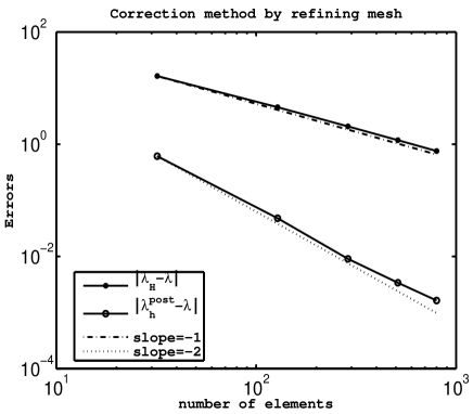
Figure 1: Errors for refining mesh method with $\alpha_{K}=0.1$

Then we give numerical results of the postprocessing algorithm which the enriched spaces constructed by one order higher finite element. We first solve the Stokes eigenvalue problem (2.10) by the lowest order stabilization element $(V_{h},D_{h})=(P_{1},P_{-1}^{\rm disc})$ and solve the Stokes source problem (6.1) by second order stabilization element $(V_{h},D_{h})=(P_{2}^{+},P_{1}^{\rm disc})$ ([25]) with

$$P_{2}^{+}= \big{\{}v\in H^{1}(\Omega):v|_{K}\in P_{2}(K)\oplus\varphi_{K}\cdot P_{1}(K),\ \forall K\in\mathcal{T}_{h}\big{\}},$$

$$P_{1}^{\rm disc}= \big{\{}v\in L^{2}(\Omega):v|_{K}\in P_{1}(K),\ \forall K\in\mathcal{T}_{h}\big{\}},$$

on the same triangular meshes, where the bubble function $\varphi_{K}$ is defined by the barycenter coordinates $\lambda_{1,K},\lambda_{2,K}$ and $\lambda_{3,K}$ on the element $K$ with $\varphi_{K}:=\lambda_{1,K}\lambda_{2,K}\lambda_{3,K}$.

The numerical results are shown in Figure 2.

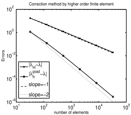
Figure 2: Errors for higher order method with $\alpha_{K}=0.1$

From Figures 1 and 2, we can find that the postprocessing algorithm can improve the accuracy of the eigenvalue approximations and confirm the theoretical analysis.

8 Concluding remarks

In this paper, the LPS method is applied to obtain the approximations of Stokes eigenvalue problem and a type of postprocessing method is also proposed to improve the convergence order for the eigenpair approximation. The theoretical analysis is given and the corresponding numerical examples are also used to confirm the analysis. The postprocessing method proposed here can be coupled with the adaptive mesh refinement in the two-grid method. The application of LPS method makes the implementation of adaptive mesh refinement more easily for solving Stokes eigenvalue problems especially on the meshes with hanging nodes ([32]).

In the future, we will extend our postprocessing method to the nonsymmetric Stokes eigenvalue problems which is more general in the study of linearized stability for the Navier-Stokes equations ([21]).

References

[1]
A. B. Andreev, R. D. Lazarov and M. R. Racheva, Postprocessing and
higher order convergence of the mixed finite element approximations
of biharmonic eigenvalue problems, J. Comput. Appl. Math.,
182(2005), 333-349.
[2]
I. Babuška and J. E. Osborn, Finite element-Galerkin
approximation of the eigenvalues and eigenvectors of selfadjoint
problems, Math. Comp. 52(1989), 275-297.
[3]
I. Babuška and J. Osborn, Eigenvalue Problems, In Handbook of
Numerical Analysis, Vol. II, (Eds. P. G. Lions and Ciarlet P.G.),
Finite Element Methods (Part 1), North-Holland, Amsterdam, 641-787,
1991.
[4]
C. Bacuta and J. H. Bramble, Regularity estimates for the solutions
of the equations of linear elasticity in convex plane polygonal
domain, Special issue dedicated to Lawrence E. Payne, Z. Angew.
Math. Phys., 54 (2003), 874-878.
[5]
C. Bacuta, J. H. Bramble and J. E. Pasciak, Shift theorems for the
biharmonic Dirichlet problem, Recent Progress in Computational and
Appl. PDEs, proceedings of the International Symposium on
Computational and Applied PDEs, Kluwer Academic/Plenum Publishers,
2001.
[6]
P. F. Batcho and G.E.M. Karniadakis, Generalized Stokes eigenfunctions:
a new trial basis for the solution of the incompressible Navier-Stokes equations,
J. Comput. Phys., 115(1994), 121-1146.
[7]
R. Becker and M. Braack, A finite element pressure gradient
stabilization for the Stokes equations based on local projections,
Calcolo, 38(2001), 173-199.
[8]
R. Becker and M. Braack, A two-level stabilization scheme for the
Navier-Stokes equations, in Numerical Mathematics and Advanced
Aplications, M. Feistauer, et al, eds., Springer, Berlin, 2004,
123-130.
[9]
H. Blum and R. Rannacher, On the boundary value problem of the
biharmonic operator on domains with singular corners, Math. Meth. in
the Appl. Sci., 2 (1980), 556-581.
[10]
M. Braack and E. Burman, Local projection stabilization for the
Oseen problem and its interpretation as a variational multiscale
method, SIAM J. Numer. Anal., 43(6)(2006), 2544-2566.
[11]
S. Brenner and L. Scott, The Mathematical Theory of Finite Element
Methods, New York: Springer-Verlag, 1994.
[12]
F. Brezzi and M. Fortin, Mixed and Hybrid Finite Element
Methods, New York: Springer-Verlag, 1991.
[13]
F. Chatelin, Spectral Approximation of Linear Operators, Academic
Press Inc, New York, 1983.
[14]
W. Chen and Q. Lin, Approximation of an eigenvalue problem
associated with the Stokes problem by the stream
function-vorticity-pressure method, Appl. Math., 51(1)(2006),
73-88.
[15]
H. Chen, S. Jia and H. Xie, Postprocessing and higher order
convergence for the mixed finite element approximations of the
Stokes eigenvalue problems, Appl. Math., 54(3)(2009), 237-250.
[16]
P. G. Ciarlet, The finite Element Method for Elliptic Problem,
North-holland Amsterdam, 1978.
[17]
P. Clement, Approximation by finite element functions using local regularization, RAIRO Anal. Numer.,
9(1975), 77-84.
[18]
E. B. Fabes, C. E. Kenig and G. C. Verchota, The Dirichlet problem
for the Stokes system on Lipschitz domains, Duke Math. J., 57
(1998), 769-793.
[19]
S. Ganesan, G. Matthies and L. Tobiska, Local projection
stabilization of equal order interpolation applied to the Stokes
probelm, Math. Comp., 77(264)(2008), 2039-2060.
[20]
V. Girault and P. Raviart, Finite Element Methods for Navier-Stokes
Equations, Theory and Algorithms, Springer-Verlag, Berlin, 1986.
[21]
V. Heuveline and R. Rannacher, Adaptive FEM for eigenvalue problems
with application in hydrodynamic stability analysis, J. Numer.
Math., 0(0)(2006), 1-32.
[22]
E. Leriche and G. Labrosse, Stokes eigenmodes in square domain and the stream function-vorticity correlation,
J. Comput. Phys., 200(2004), 489-511.
[23]
Q. Lin and N. Yan, The Construction and Analysis of High Efficiency Finite Element Methods,
HeBei University Publishers, 1995.
[24]
C. Lovadina, M. Lyly 3 and R. Stenberg 4, A posteriori estimates for the Stokes eigenvalue problem,
Numer. Methods Partial Differential Equations, 25(1)(2008), 244 - 257.
[25]
G. Matthies, P. Skrzypacz and L. Tobiska, A unified convergence
analysis for local projection stabilizations applied to the Oseen
problem, M2AN Math. Model. Numer. Anal., 41(2007), 713-742.
[26]
G. Matthies, P. Skrzypacz, and L. Tobiska. Stabilization of local
projection type applied to convection-diffusion problems with mixed
boundary conditions, ETNA, 32(2008), 90-105.
[27]
B. Mercier, J. Osborn, J. Rappaz and P.A. Raviart, Eigenvalue
approximation by mixed and hybrid methods, Math. Comput., 36 (154)
(1981), 427-453.
[28]
K. Nafa and A.J. Wathen, Local projection stabilized Galerkin
approximations for the generalized Stokes problem, Comput. Methods
Appl. Mech. Engrg., 198(2009), 877-833.
[29]
J. Osborn, Approximation of the eigenvalue of a nonselfadjoint
operator arising in the study of the stability of stationary
solutions of the Navier-Stokes equations, SIAM J. Numer. Anal., 13
(1976), 185-197.
[30]
M. R. Racheva and A. B. Andreev, Superconvergence postprocessing for
Eigenvalues, Comp. Methods in Appl. Math., 2(2)(2002), 171-185.
[31]
H.-G. Roos, M. Stynes, and L. Tobiska, Robust numerical methods for singularly perturbed
differential equations. Convection-diffusion-reaction and flow problems, Number 24 in SCM.
Springer, Berlin, 2008.
[32]
F. Schieweck, Uniformly stable mixed hp-finite elements on
multilevel adaptive grids with hanging nodes, Math. Model. Numer.
Anal. M2AN, 42(2008), 493-505.
[33]
L. R. Scott and S. Zhang, Finite element interpolation of nonsmooth functions satisfying boundary
conditions, Math. Comp., 54(190)(1990), 483-493.
[34]
C. Wieners, A numerical existence proof of nodal lines for the first
eigenfunction of the plate equation, Arch. Math. 66(1996),
420-427.
[35]
J. Xu and A. Zhou, A two-grid discretization scheme for eigenvalue
problems, Math. of Comput., 70(233)(2001), 17-25.