Influence of phonons on exciton-photon interaction and photon statistics of a quantum dot

Abstract

In this paper, we investigate, phonon effects on the optical properties of a spherical quantum dot. For this purpose, we consider the interaction of a spherical quantum dot with classical and quantum fields while the exciton of quantum dot interacts with a solid state reservoir. We show that phonons strongly affect the Rabi oscillations and optical coherence on first picoseconds of dynamics. We consider the quantum statistics of emitted photons by quantum dot and we show that these photons are anti-bunched and obey the sub-Poissonian statistics. In addition, we examine the effects of detuning and interaction of quantum dot with the cavity mode on optical coherence of energy levels. The effects of detuning and interaction of quantum dot with cavity mode on optical coherence of energy levels are compared to the effects of its interaction with classical pulse.

I Introduction

The fundamental system in cavity quantum electrodynamics (cavity-QED) is a two level atom interacting with a single-cavity mode qo1 -qo2 . Recent developments in semiconductor nano-technology have shown that excitons in quantum dots (QDs) constitute an alternative two-level system for cavity-QED application gerard . There are many similarities between the excitons in QDs and atomic systems, such as the discrete level structures which is subsequent of three-dimensional confinement of electrons. On the other hand, there are also important differences, for example coupling to phonons, carrier-carrier interaction and surface fluctuation. Coupling of electrons to phonons plays a major role in QDs. The coupling of phonons to the QD provides a basic dephasing mechanism and thus marks a lower limit for the decoherence mulj -knorr . In self-assembled QDs it is indeed the elastic phonon scattering (pure dephasing) which dominates the loss of coherence on a picosecond time scale at temperatures below $100$K borri . The effects of electron-phonon interactions on strong exciton-photon coupling in cavity-QED has been considered wilson . It has been shown vagov2 that the phonon-induced damping of Rabi oscillations in a QD is a non-monotonic function of the laser-field intensity that is increasing at low fields and decreasing at high fields.
QDs are also promising candidates for efficient, deterministic single photon sources shield -santor . Then the QDs are important sources of non-classical light. For this kind of application an understanding of the coherence properties of its optical transitions is of great importance. Therefore, there are two processes in optical manipulation with semiconductor QDs: coherent control of the QD exciton state axt and measurement of quantum statistics of emitted light with QD muller . A theoretical investigation of exciton dynamics and the possibility of generation of non-classical light has been considered without taking into account the phonon effects perea .
In this paper, we investigate the effects of electron-phonon interactions on optical coherence and quantum statistics of light emitted by a pulse driven QD interacting with a cavity mode. The photon statistics from a driven QD under the influence of the phonon environment has been considered recently zahir . On the other hand, influence of phonons on incoherent photon emission of a QD in the presence of pulse excitation had been considered ahn . We use the most widely studied model for phonon effects in QDs which accounts two electronic levels coupled to a laser pulse and to non-interacting phonons machni . As mentioned, phonon interaction provides a dephasing mechanism for optically induced coherence on a time scale (a few picosecond) much shorter than for radiative interaction and recombination borri1 . Due to the different correlation time for a phonon reservoir (few picosecond) and for a radiative reservoir (several ten nanosecond) we restrict our attention to the time scales which dephasing effects due to the phonon system play an important role (with the radiative reservoir we mean a reservoir for photon system. The mentioned time scale relates to the decay time of cavity photons). Then we do not consider any damping effect on cavity mode and spontaneous emission. In our consideration the only damping effect is related to phonons.
The paper is organized as follows: In section II we describe the model Hamiltonian and master equation that allows to calculate the evolution of populations and coherence of the energy levels. In section III we present the exciton dynamics and its coherence while driven with a laser pulse. The photon statistics and exciton dynamics of pulse driven QD interacting with a cavity mode is presented and discussed in section IV. Section V is devoted to a summery and conclusion.

II Theoretical model

We consider a single QD inside a semiconductor microcavity that is pumped with a laser pulse and interacts with a cavity mode. It is assumed that the system is initially prepared in its ground state. We consider a solid-state reservoir for the exciton population and we focus on time scales which phonon effects are important. We neglect other sources of damping in the system. We model the QD by a two-level system with ground state $|g\rangle$ (the semiconductor ground-state) and first excited state $|e\rangle$ (a single exciton), separated by an energy $\hbar\omega_{ex}$. The phonon environment is modelled by a bath of harmonic oscillators of frequencies $\omega_{k}$, with the wavevector $k$. The Hamiltonian of the total system in the rotating wave approximation is written as

$$\hat{H} = \hbar\omega_{ex}\hat{\sigma}_{ee}+\hbar\omega_{c}\hat{a}^{{\dagger}}\hat{a}+\sum_{k}\hbar\omega_{k}\hat{b}^{{\dagger}}_{k}\hat{b}_{k}$$ (1)

$$+ \hbar g(\hat{\sigma}_{eg}\hat{a}+\hat{a}^{{\dagger}}\hat{\sigma}_{ge})+\hbar f(t)(\hat{\sigma}_{eg}+\hat{\sigma}_{ge})$$

$$+ \hat{\sigma}_{ee}\sum_{k}\lambda_{k}(\hat{b}_{k}+\hat{b}^{\dagger}_{k}),$$

where $\hat{\sigma}_{ij}=|i\rangle\langle j|$, $\hat{a}\;(\hat{a}^{\dagger})$ and $\hat{b}_{k}\;(\hat{b}^{\dagger}_{k})$ are the annihilation (creation) operators for cavity mode, and $k$th phonon mode, respectively. The parameter $g$ is the coupling constant of the exciton and cavity mode, and $f(t)$ is a real envelope function of the driving pulse. The last term in the Hamiltonian describes the exciton-phonon interaction. In this term, $\lambda_{k}$ is the corresponding coupling constant. The coupling of the confined exciton to the acoustic phonons by means of the deformation potential tends to dominant the dephasing dynamics, over the piezoelectric interaction or coupling to optical phonons krumm . In this case, the coupling constant is given by $\lambda_{k}=kD(k)\sqrt{2n\omega_{k}V}$ mahan where $n$ is the sample density and $V$ is the unit cell volume. $D(k)$ is the form factor of the confined electron and hole in the ground state of the QD. The Hamiltonian in the interaction picture can be written as

$$\hat{H}_{int}=\hat{H}_{0}+\hat{H}_{R},$$ (2)

where we decompose the coherent-field part and environment part as follow

$$\hat{H}_{0} = \hbar g(\hat{\sigma}_{eg}\hat{a}e^{i\Delta t}+\hat{a}^{{\dagger}}\hat{\sigma}_{ge}e^{-i\Delta t})$$

$$+ \hbar f(t)(\hat{\sigma}_{eg}e^{i\omega_{ex}t}+\hat{\sigma}_{ge}e^{-i\omega_{ex}t}),$$

$$\hat{H}_{R} = \hat{\sigma}_{ee}\sum_{k}\lambda_{k}(\hat{b}_{k}e^{-i\omega_{k}t}+\hat{b}^{{\dagger}}e^{i\omega_{k}t}).$$ (3)

In this equation $\Delta=\omega_{ex}-\omega_{c}$ is detuning between the exciton excitation energy in the QD and cavity field energy.
Now we consider the Liouville equation of density matrix in the interaction picture

$$\frac{d\hat{\rho}_{t}}{dt}=\frac{i}{\hbar}[\hat{\rho}_{t},\hat{H}_{int}].$$ (4)

We define the reduced density matrix $\hat{\rho}$ for the exciton-photon system by tracing out the phonon degrees of freedom in the total density matrix, $\hat{\rho}=Tr_{ph}(\hat{\rho}_{t})$. Now we consider the master equation in the Born approximation qo1 -qo2 in the case of the phonon interaction while we consider the gain and pump parts exactly. Phonons are one of the slowest process and this kind of reservoir has a correlation time of the order of a few picosecond krumm and this reservoir is naturally non-Markovian. To consider non-Markovian dynamics we have used time convolutionless projection operator method bruer , up to second order of expansion. We assume an uncorrelated state for initial state of the exciton-photon system and phonon reservoir. At the initial time $t=0$ the phonon system is assumed to be in a thermal equilibrium at temperature $T$. Then the density operator of the exciton-photon system satisfies the following dynamical equation

$$\dot{\rho}(t) = \frac{i}{\hbar}[\rho(t),\hat{H}_{0}]-\int_{0}^{t}([\hat{\sigma}_{ee},\hat{\sigma}_{ee}\rho(t)]K(t-t^{\prime})$$ (5)

$$- [\hat{\sigma}_{ee},\rho(t)\hat{\sigma}_{ee}]K^{\ast}(t-t^{\prime}))dt^{\prime}.$$

The first term describes the coherent evolution of the density matrix $\rho$ under the action of the Hamiltonian $\hat{H}_{0}$ of the dot-cavity-pulse system. The kernel $K$ which is the correlation function of the environment is written as

$$K(t)=\frac{1}{\hbar^{2}}\int_{0}^{\infty}d\omega j(\omega)\left[coth(\frac{\hbar\omega}{2k_{B}T})cos(\omega t)-isin(\omega t)\right],$$ (6)

with Boltzmann constant $k_{B}$. $j(\omega)$ is the spectral density of the phonons which completely describes the interaction of exciton and phonons weiss . Here, we introduce the following spectral density

$$j(\omega)=\sum_{k}\lambda_{k}^{2}\delta(\omega-\omega_{k}).$$ (7)

The density matrix dynamics is obtained under the Born-Markov approximation for exciton-phonon interaction and the strong exciton-photon interaction and pump effects are described exactly. We can extract exciton dynamics and photon statistics from this equation.

III Exciton dynamics under a driving pulse

In this section we consider the optical coherence of a driven QD under a pump pulse. Here we neglect the cavity mode and we consider optical coherence and exciton population dynamics under pulse excitation and effects of physical parameters such as pulse duration on these physical quantities. Then the density matrix of the excitonic system satisfies the following equation of motion

$$\dot{\rho}_{ex}(t) = \frac{i}{\hbar}[\rho_{ex}(t),\hbar(\hat{\sigma}_{eg}\alpha(t)+\hat{\sigma}_{ge}\alpha^{\ast}(t))]$$

$$- \int_{0}^{t}([\hat{\sigma}_{ee},\hat{\sigma}_{ee}\rho(t)]K(t-t^{\prime})$$

$$- [\hat{\sigma}_{ee},\rho(t)\hat{\sigma}_{ee}]K^{\ast}(t-t^{\prime}))dt^{\prime},$$ (9)

where $\alpha(t)=f(t)e^{i\omega_{ex}t}$. Exciton population and optical induced coherence in the QD system are defined through the different matrix elements of the density matrix. Exciton population and optical coherence are defined with the following set of equations, respectively

$$\dot{P}(t) = i\alpha(t)(2N_{e}(t)-1)-P(t)\int_{0}^{t}K(t-t^{\prime})dt^{\prime},$$

$$\dot{N}_{e}(t) = 2iIm(\alpha^{\ast}(t)P(t)),$$ (10)

where $P(t)=\langle e|\hat{\rho}_{ex}(t)|g\rangle$ and $N_{e}(t)=\langle e|\hat{\rho}_{ex}(t)|e\rangle$. We assume at $t=0$ the QD be in its ground state and at this time it is excited with a Gaussian pulse excitation with envelop function $f(t)=\frac{A}{\sqrt{2\pi}a}e^{-\frac{t^{2}}{a^{2}}}$ where $a$ is the pulse width and $A$ is a measure of pulse amplitude. For numerical integration of this set of equations, we shall take a GaAs QD with a spherical shape. In this case the spectral density is given by

$$j(\omega)=\frac{(\sigma_{e}-\sigma_{h})^{2}}{4\pi^{2}\rho c^{5}}\omega^{3}e^{-\frac{3l^{2}}{2c^{2}}\omega^{2}},$$ (11)

where $\sigma_{e}$ and $\sigma_{h}$ are the bulk deformation potential constants for electron and hole, $c$ is the sound velocity in the sample and $l$ is the electron and hole ground-state localization length (we assume a spherically symmetric harmonic confinement potential for the QD and electron and hole in the ground state). We use the following numerical values $\sigma_{e}-\sigma_{h}=9eV$, $\rho=5350\frac{kg}{m^{3}}$, $c=5150\frac{m}{s}$ and $l=4.5nm$ (these material parameters are approximately acquired from amk ). Figure (1) shows plots of the time evolution of the exciton inversion for two values of pulse duration. In first picoseconds of dynamics the time evolution shows a strong decrease of exciton inversion due to the phonon effects and then we see a stable oscillation in inversion behavior during the pulse duration. It is clear from the figure that the phonon effects can prevent exciton generation. On the other hand, we see the complex behavior on the same timescales of initial dynamics for each pulse duration and after that small oscillations will continue at the end of pulse duration. Then we conclude that in the first steps of dynamics the influence of phonons is a very important damping effect. Figure(2) shows plots of $ImP(t)$ to consider the time evolution of optical coherence. As in the case of exciton population, optical coherence experiences a very rapid decrease during some first picoseconds. After this strong decrease we see a very small stable oscillations in optical coherence. Therefore, we concloud phonon effects are very important on timescales smaller than the spontaneous decay time and we can consider phonon reservoir as dominant damping source during the first steps of dynamics.

IV Interaction of QD with cavity mode

In this section we consider the interaction of the QD embedded in a microcavity with cavity mode. In this case, the density matrix for the system satisfies Eq.(5). By using Eq.(5) one can get a set of differential equations that describe the evolution of the populations and coherence of the cavity-QD system. In the basis of product states between the QD states and Fock states of the cavity mode ($|en\rangle$, $|gn\rangle$) we calculate the matrix elements of the exciton-photon density matrix. By taking the matrix elements in Eq.(5) we get the following set of linear differential equations for the populations and coherence in the QD-photon system (we have used the notation $\rho_{in,jm}=\langle in|\rho|jm\rangle$ in which $i$ and $j$ refer to QD states)

$$\dot{\rho}_{en-1,en-1}(t)=ig\sqrt{n}(\rho_{en-1,gn}(t)e^{-i\Delta t}-\rho_{gn,en-1}(t)e^{i\Delta t})$$

$$+if(t)(\rho_{en-1,gn-1}(t)e^{-i\omega_{ex}t}-\rho_{gn-1,en-1}(t)e^{i\omega_{ex}t}),$$ (12a)

$$\dot{\rho}_{gn,gn}(t)=ig\sqrt{n}(\rho_{gn,en-1}(t)e^{i\Delta t}-\rho_{en-1,gn}(t)e^{-i\Delta t})$$

$$+if(t)(\rho_{gn,en}(t)e^{i\omega_{ex}t}-\rho_{en,gn}(t)e^{-i\omega_{ex}t}),$$ (12b)

$$\dot{\rho}_{en-1,gn}(t)=ig\sqrt{n}(\rho_{en-1,en-1}(t)e^{i\Delta t}$$

$$-\rho_{gn,gn}(t)e^{i\Delta t})-\rho_{en-1,gn}(t)\int_{0}^{t}K(t-t^{\prime})dt^{\prime},$$ (12c)

$$\dot{\rho}_{en-1,gn-1}(t)=if(t)(\rho_{en-1,en-1}(t)e^{i\omega_{ex}t}$$

$$-\rho_{gn-1,gn-1}(t)e^{i\omega_{ex}t})-\rho_{en-1,gn-1}(t)\int_{0}^{t}K(t-t^{\prime})dt^{\prime}.$$ (12d)

In the absence of pulse excitation, the matrix elements $\rho_{en-1,en-1}(t)$, $\rho_{gn,gn}(t)$, $\rho_{en-1,gn}(t)$ and $\rho_{gn,en-1}(t)$, for a given photon number, satisfy a closed set of differential equations. However, the excitation pulse couples the different terms to each other and an infinite set of equations has to be solved. In the process of obtaining the above set of equations we neglect the terms like $\rho_{gn,gn-1}(t)$ and $\rho_{en,en-1}(t)$ because these terms do not have physical meaning related to the conditions under consideration. These terms show a coherence in photon field while the QD remains in its state. This could be related to photon damping which we have neglected such kind of terms. On the other hand, we maintain terms like $\rho_{en,gn}(t)$ which describe coherence in QD system while photon number is constant. As is clear from (12) these terms cam be generated during the dynamics by the pump pulse.
As initial condition we take at $t=0$ the QD in its ground state and cavity field in the vacuum state $\rho_{g0,g0}(0)=1$, and all other elements of the density matrix equal to zero. For the numerical integration, the set of equations can be truncated at a given value, which we take it equal to 90 (this value is choose with this condition that the results not change with increasing the number of equation).
Photon statistics and material characteristics such as inversion population and optical coherence can be obtained from (12). At first we consider Mandel parameter of the cavity field which is defined as mandel

$$M=\frac{\langle\hat{n}^{2}\rangle-\langle\hat{n}\rangle^{2}}{\langle\hat{n}\rangle}-1.$$ (13)

This parameter vanishes for the Poisson distribution, is positive for the super-Poisson distribution (photon bunching effect), and is negative for the sub-Poisson distribution (photon anti-bunching effect). The mean number of photons in the cavity is (other moments of $\hat{n}$ can be calculated in the same manner)

$$\langle\hat{n}\rangle=\sum_{n}n\left[\rho_{en,en}(t)+\rho_{gn,gn}(t)\right].$$ (14)

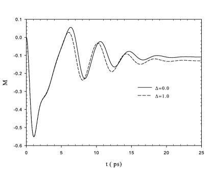
Figure 3: Mandel parameter versus time for pulse duration $a=10ps$ and $T=30K$ for two different values of detuning $\Delta=0.0,\;\Delta=1.0$.

Mandel parameter for the case of resonant interaction ($\Delta=0$) and in the presence of detuning is plotted, respectively, in figures (3) and (4) for two different values of pulse duration. As is seen, the cavity field mode exhibits non-classical (sub-Poissonian statistics) in the course of time evolution. Another important feature of this plot is the oscillatory behavior of Mandel parameter for time scales approximately two times of pulse duration. Therefore, the emitted photons to cavity mode by QD in the course of the excitation duration can be reabsorbed by QD and re-excite the QD then after the end of pulse duration we have oscillations in photon statistics. On the other hand, it is clear that with increasing the detuning feature the amplitude of oscillations in Mandel parameter decrease.
Another important quantity in photon statistics is second order coherence function, $g^{(2)}(t,\tau)$ qo1 ,mandel which is a two-time correlation function. Here we consider this quantity for the case of zero time delay, $g^{(2)}(t,\tau=0)$. This quantity can be used as an indication of the possible coherence of the state of the photon system. For the single mode cavity field $g^{(2)}(t,\tau=0)$ has the following definition

$$g^{(2)}(t,\tau=0) = \frac{\langle a^{\dagger}a^{\dagger}aa\rangle}{\langle a^{\dagger}a\rangle^{2}}$$

$$= \frac{\sum_{n}n(n-1)\left[\rho_{en,en}(t)+\rho_{gn,gn}(t)\right]}{\left(\sum_{n}n\left[\rho_{en,en}(t)+\rho_{gn,gn}(t)\right]\right)^{2}}.$$

In the case of resonant interaction and off-resonant interaction, the plots of this quantity are shown in figures(5) and (6), respectively. The figures show non-classical nature of emitted photons (photon anti-bunching). This quantity shows similar oscillatory behavior to the Mandel parameter and its oscillatory behavior continue up to times twice the pulse duration. According to these plots the detuning effects on $g^{(2)}(t,\tau=0)$ are similar to its effects on the Mandel parameter and cause the amplitude of oscillation be reduced. Therefore, in this conditions without any restriction on physical parameters (damping coefficients and coupling constant) it is possible that QD emits anti-bunched photons with sub-Poissonian statistics. The possibility of emitting anti-bunched photons with sub-Poissonian statistics by a single QD has been considered experimentally becher .
The time evolution of the QD coherence in the process of one photon interaction $P(t)=\langle e0|\rho(t)|g1\rangle$ is shown in figures(7) and (8) for different values of pulse duration and detuning. In these figures we plot imaginary part of $P(t)$. These figures indicating occurrence of decoherence (damping of the imaginary part of polarization) in the system. The main source of this decoherence is phonon interaction. In the case of pulse with long duration we see an irregular oscillation in some time periods. It is clear that detuning prevents the coherence in this system. However the detuning is increased the imaginary part of coherence $P(t)$ and increasing of detuning leads to the regular oscillatory behavior and causes damping will decrease. In turn, because of the detuning, which weakens the dynamics, the pumping should be increased. Hence these two parameter can be considered as some experimental parameters for controling the decoherence in the QD systems on the timescales under consideration. On the other hand, by comparison Fig.(2) with Fig.(7) we can conclude that while the QD interacts with a cavity mode its optical coherence between energy levels has a longer life time. Then this can be considered as another experimental condition for controlling of optical coherence.

V Conclusion

In this paper we have considered phonon effects (dephasing effects) on optical properties of a pulse driven QD. We have shown that these effects strongly affect the Rabi oscillations and optical coherence. In the time scales which spontaneous emission and non-radiative recombination do not play an important role in the dynamics (characteristic times of these effects are much longer than the characteristic time of phonon reservoir) the phonons strongly affect optical properties of QD. In the case of the interaction of system under consideration with cavity mode we have shown that emitted photons are anti-bunched and obey the sub-Poissonian statistics. Then in the microcavity with high quality factor which contains a single QD it is possible to generate non-classical light in the first some ten picoseconds. Here, we have considered a Gaussian pulse as a pump. We have shown that with the ending of pump, oscillations in the photon statistics continue until times twice the pulse duration. This relates to cavity photon which remains in the cavity and after ending of pump re-excites the QD. On the other hand, we have considered the detuning effect on the optical coherence of QD and we have seen that detuning can prevent decoherence effects. Hence, detuning can be considered as a controlling parameter of optical coherence. While QD interacts resonantly with the cavity mode, we have found that its optical coherence has a longer life time in comparison with its interaction with classical pulse. Then by putting the QD in the cavity it can maintain its coherence between energy levels. Therefore, the off-resonant interaction of a QD with cavity mode can be considered as an experimental tool for suppressing decoherence effects on the exciton.

Acknowledgment The authors wish to thank the Office of Graduate Studies of the University of Isfahan and Iranian Nanotechnology initiative for their support.

Figure 1: Plots of exciton inversion versus time for two different values of pulse duration: (a) $a=10ps$, (b) $a=40ps$. Material parameters are pointed out in the text and $T=30K$.

Figure 2: Plots of imaginary part of optical polarization versus time for two different values of pulse duration: (a) $a=10ps$, (b) $a=40ps$. Material parameters are pointed out in the text and $T=30K$.

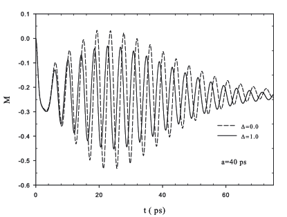
Figure 4: Mandel parameter versus time for pulse duration $a=40ps$ and $T=30K$ for two different values of detuning $\Delta=0.0,\;\Delta=1.0$.

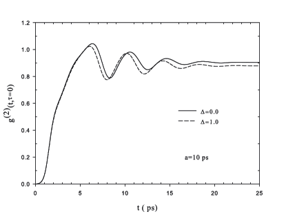
Figure 5: $g^{(2)}(t,\tau=0)$ as a function of time for pulse duration $a=10ps$ and $T=30K$ for two different values of detuning $\Delta=0.0,\;\Delta=1.0$.

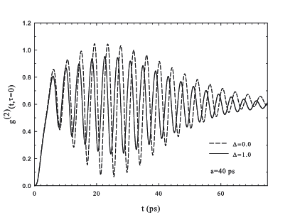
Figure 6: $g^{(2)}(t,\tau=0)$ as a function of time for pulse duration $a=40ps$ and $T=30K$ for two different values of detuning $\Delta=0.0,\;\Delta=1.0$.

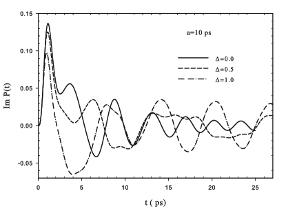
Figure 7: $ImP(t)$ as a function of time for three different values of detuning and for pulse duration $a=10ps$. In this plot $T=30K$.

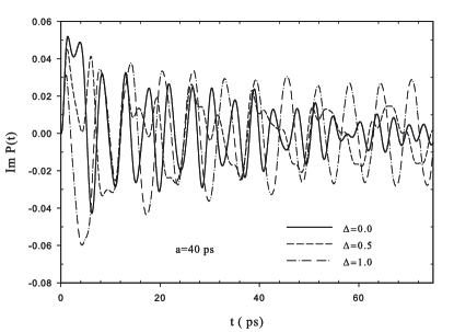
Figure 8: $ImP(t)$ as a function of time for three different values of detuning and for pulse duration $a=40ps$. In this plot $T=30K$.

References

- (1) M. O. Scully and M. S. Zubairy, Quantum Optics(Cambridge University Press, Cambridge 1997).
- (2) Y. Yamamoto and A. Imamoglu, Mesoscopic Quantum Optics, (wiley, New York, 1999).
-
(3)
J. M. Gerard, B. Sermage, B. Gayral, B. Legrand, E. Costard, and V.
Thierry-Mieg, Phys. Rev. Lett 81, 1110 (1998).
P. Michler, A. Kiraz, C. Becher, W. V. Schoenfeld, P. M. Petroff, Lidong Zhang, E. Hu, A. Imamoglu, Science 290, 2282 (2000). - (4) E. A. Muljarov, T. Takagahara, and R. Zimmermann, Phys. Rev. Lett 95, 177405 (2005).
- (5) A. Vagov, V. M. Axt, and T. Kuhn, Phys. Rev. B 66 165312 (2002).
- (6) J. Förstner, C. Weber, J. Danckwerts, and A. Knorr, Phys. Rev. Lett 91, 127401 (2003).
- (7) P. Borri, W. Langbein, U. Woggon, V. Stavarache, D. Reuter, and A. D. Wieck, Phys. Rev. B 71, 115328 (2005).
- (8) I. Wilson-Rae, and A. Imamoglu, Phys. Rev. B 65, 235311 (2002).
- (9) A. Vagov, M. D. Croitoru, V. M. Axt, T. Kuhn, and F. M. Peeters, Phys. Rev. Lett 98, 227403 (2007).
- (10) Andrew J. Shields, Nature Photonics 1, 215 (2007).
- (11) C. Santori, D. Fattal, J. Vuckovic, G. S. Solomon, and Y. Yamamoto, Nature 419, 594 (2002).
- (12) V. M. Axt, P. Machnikowski, and T. Kuhn, Phys. Rev. B 71, 155305 (2005).
- (13) A. Muller, E. B. Flagg, P. Bianucci, D. G. Deppe, W. Ma, J. Zhang, G. J. Salamo, and C. K. Shih, arXiv: 0707.3808 (2007).
- (14) J. I. Perea, D. Porras, and C. Tejedor, Phys. Rev. B 70, 115304 (2004).
- (15) A. Nazir, Phys. Rev. B 78, 153309 (2008).
- (16) K. J. Ahn, J. Förstner, and A. Knorr, phys. Rev. B 71, 153309 (2005).
- (17) P. Machnikowski, and L. Jacak, Phys. Rev. B 69, 193302 (2004).
-
(18)
P. Borri, W. Langbein, S. Schneider,
U. Woggon, R. L. Sellin, D. Ouyang, and D. Bimberg, Phys. Rev.
Lett. 87, 157401 (2001).
A. Vagov, V. M. Axt, and T. Kuhn, Phys. Rev. B 67, 115338 (2003). -
(19)
B. Krummheuer, V. M. Axt, and T. Kuhn, Phys. Rev. B 65, 195313
(2002).
E. Pazy, Semicond. Sci. Technol. 17, 1172 (2002). - (20) H.-P. Breuer, and F. Petruccione, The Theory of Open Quantum Systems(Oxford University Press, 2002).
- (21) G. Mahan, Many-Body Physics (Kluwer, New York, 2000).
- (22) U. Weiss, Quantum Dissipative Systems (WOrld Scientific, Singapore, 1999).
- (23) V. M. Axt, P. Machnikowski, T. Kuhn, Phys. Rev. B 71, 155305 (2005).
- (24) L. Mandel and E. Wolf, Optical Coherence and Quantum Optics (Cambridge University Press 1995).
- (25) C. Becher, A. Kiraz, P. Michler, A. Imamoglu, W. V. Schoenfeld, P. M. Petroff, L. Zhang, and E. Hu, Phys. Rev. B 63, 121312(R) (2001).