Analysis of reflection coefficients for the Fokker-Planck equation

Abstract

Mathematical structure of the reflection coefficients for the one-dimensional Fokker-Planck equation is studied. A new formalism using differential operators is introduced and applied to the analysis in high- and low-energy regions. Formulas for high-energy and low-energy expansions are derived, and expressions for the coefficients of the expansion, as well as the remainder terms, are obtained for general forms of the potential. Conditions for the validity of these expansions are discussed on the basis of the analysis of the remainder terms.

1 Introduction

It is well known that the steady-state Schrödinger equation

$$-\frac{d^{2}}{dx^{2}}\psi(x)+V_{\rm S}(x)\psi(x)=k^{2}\psi(x)$$ (1.1)

is equivalent to the Fokker-Planck eigenvalue equation [1]

$$-\frac{d^{2}}{dx^{2}}\phi(x)+2\frac{d}{dx}[f(x)\phi(x)]=k^{2}\phi(x).$$ (1.2)

The time-dependent Fokker-Planck equation corresponding to (1.2) describes diffusion in a potential $V(x)$, where

$$f(x)=-\frac{1}{2}\frac{d}{dx}V(x).$$ (1.3)

The correspondence between (1.1) and (1.2) is given by

$$\psi(x)=e^{V(x)/2}\phi(x),\qquad V_{\rm S}(x)=f^{\prime}(x)+f^{2}(x).$$ (1.4)

We define the transmission and reflection coefficients for a finite interval $(x_{1},x_{2})$ as follows. Let $\bar{V}(x)$ be the function which is identical with $V(x)$ inside the interval $(x_{1},x_{2})$ and constant outside:

$$\bar{V}(x)=\cases{V(x_{1})&$x\leq x_{1}$\\ V(x)&$x_{1}<x<x_{2}$\\ V(x_{2})&$x_{2}\leq x$}.$$ (1.5)

We define $\bar{f}(x)\equiv-(1/2)(d/dx)\bar{V}(x)$ just like (1.3), and consider equation (1.2) with $f(x)$ replaced by $\bar{f}(x)$. (In general, delta functions appear at $x=x_{1}$ and $x=x_{2}$ on the left-hand side of this equation.) Since $\bar{f}(x)=0$ outside $(x_{1},x_{2})$, this equation has two independent solutions of the form

$$\phi_{1}(x)=\cases{e^{ik(x-x_{1})}+R_{l}(x_{2},x_{1};k)\,e^{-ik(x-x_{1})}&$x<x_{1}$\\ e^{-[V(x_{2})-V(x_{1})]/2}\tau(x_{2},x_{1};k)\,e^{ik(x-x_{2})}&$x>x_{2}$},$$ (1.6a)

$$\phi_{2}(x)=\cases{e^{[V(x_{2})-V(x_{1})]/2}\tau(x_{2},x_{1};k)\,e^{-ik(x-x_{1})}&$x<x_{1}$\\ e^{-ik(x-x_{2})}+R_{r}(x_{2},x_{1};k)\,e^{ik(x-x_{2})}&$x>x_{2}$}.$$ (1.6b)

This defines the transmission coefficient $$\tau R_{r} R_{l} (x_{1},x_{2}) e^{\pm[V(x_{2})-V(x_{1})]/2} \tau e^{V(x)/2} \psi_{1}(x)\equiv e^{[V(x)-V(x_{1})]/2}\phi_{1}(x) \psi_{2}(x)\equiv e^{[V(x)-V(x_{2})]/2}\phi_{2}(x) \psi_{1} \psi_{2} \psi_{1} \psi_{2}$$, the right reflection coefficient , and the left reflection coefficient for the interval . The factor in front of in the above equations comes from the factor in the first equation of (1.4). If we define and , then and are two independent solutions of the corresponding Schrödinger equation. Equations (1.6a) and (1.6b) can be rewritten in terms of and as

$$\psi_{1}(x)=\cases{e^{ik(x-x_{1})}+R_{l}(x_{2},x_{1};k)\,e^{-ik(x-x_{1})}&$x<x_{1}$\\ \tau(x_{2},x_{1};k)\,e^{ik(x-x_{2})}&$x>x_{2}$},$$ (1.6c)

$$\psi_{2}(x)=\cases{\tau(x_{2},x_{1};k)\,e^{-ik(x-x_{1})}&$x<x_{1}$\\ e^{-ik(x-x_{2})}+R_{r}(x_{2},x_{1};k)\,e^{ik(x-x_{2})}&$x>x_{2}$},$$ (1.6d)

in agreement with the standard definition of the transmission and reflection coefficients. Many properties of equation (1.2) or equation (1.1) can be known from these scattering coefficients.

Our object of study in this paper is the reflection coefficients for semi-infinite intervals, $R_{r}(x,-\infty;k)$ and $R_{l}(\infty,x;k)$, which play particularly important roles in one-dimensional problems. When considering a problem on the entire line in one dimension, $-\infty<x<+\infty$, we are obliged to deal with semi-infinite intervals. For example, the Green function is expressed in terms of $R_{r}(x,-\infty;k)$ and $R_{l}(\infty,x;k)$. Let $G_{\rm S}(x,x^{\prime};k)$ be the Green function for the Schrödinger equation (1.1), satisfying

$$\left[\frac{\partial^{2}}{\partial x^{2}}-V_{\rm S}(x)+k^{2}\right]G_{\rm S}(x,x^{\prime};k)=\delta(x-x^{\prime})$$ (1.6g)

with the boundary condition $G_{\rm S}(x,x^{\prime};k+i\epsilon)\to 0$ as $|x-x^{\prime}|\to\infty$. (Here $k$ is real and $\epsilon$ is a positive infinitesimal.) This Green function can be expressed as

$$G_{\rm S}(x,x^{\prime};k)=\frac{-i}{2k\sqrt{[1-S(x;k)][1-S(x^{\prime};k)]}}\exp\left[ik(x-x^{\prime})-ik\int_{x^{\prime}}^{x}S(z;k)\,dz\right]$$ (1.6h)

for $x\geq x^{\prime}$, where

$$S(x;k)\equiv\frac{R_{l}(\infty,x;k)}{1+R_{l}(\infty,x;k)}+\frac{R_{r}(x,-\infty;k)}{1+R_{r}(x,-\infty;k)}.$$ (1.6i)

Therefore, analytic properties of the Green function for the Schrödinger equation can be known by studying $R_{r}(x,-\infty;k)$ and $R_{l}(\infty,x;k)$ for the Fokker-Planck equation.

In this paper we investigate the behavior of these reflection coefficients in high-energy (large-$|k|$) and low-energy (small-$|k|$) regions. We shall deal only with $R_{r}(x,-\infty;k)$ since $R_{l}$ has the same structure as $R_{r}$. We assume that $k$ is, in general, a complex number with ${\rm Im}\,k\geq 0$.

The analysis of scattering coefficients for the Schrödinger equation has a very long history [2–4]. Even recently, the high- and low-energy asymptotic expansions of the reflection coefficients and related quantities continue to be studied actively by many researchers [5–10]. On the other hand, although the equivalence between the Schrödinger equation and the Fokker-Planck equations has been well known for a long time, little attention has been paid to the reflection coefficients for the Fokker-Planck equation. Actually, the structure of the reflection coefficients is more transparent for the Fokker-Planck equation than for the Schrödinger equation. By dealing with the Fokker-Planck equation rather than the Schrödinger equation, we can carry out the analysis in a more systematical way, as we shall see in this paper.

Conventional methods used for the Schrödinger equation mostly involve estimating a solution of an integral equation. In this paper we take a totally different approach. It is a characteristic of the reflection coefficients (and related quantities such as the Weyl $m$-function) that they satisfy a nonlinear differential equation of Riccati type. In our method, the Riccati equation is transformed into a linear partial differential equation for two variables, and the derivation of the asymptotic expansions is reduced to a manipulation of linear operators. In this method, the high-energy expansion and the low-energy expansion can be treated on an equal footing.

In studying an asymptotic expansion, it is essential to estimate the remainder term. In conventional methods, this procedure often calls for a severe restriction on the potential, requiring it to belong to a certain limited class such as $L^{1}$, $L^{2}$, or the Faddeev class. In our method, the remainder term is expressed in a fairly compact form which is valid even if the potential is infinite at $x=\pm\infty$. As a result, this method is applicable to a much larger class of potentials.

The potential $V(x)$ is a real function of $x$. (In this paper we always use the term “potential” to mean the Fokker-Planck potential $V(x)$, not the Schrödinger potential $V_{\rm S}(x)$.) Since we shall deal only with $R_{r}(x,-\infty;k)$, the potential need not be defined on the entire line. We assume that $V(x)$ is defined in $-\infty<x<x_{\rm max}$ with some $x_{\rm max}$, and that $V(x)$ takes a finite value for each $x$ in this region. (For example, $x_{\rm max}=0$ for $V(x)=\log|x|$. If the potential is defined everywhere, then $x_{\max}=+\infty$.)

We shall allow $V(x)$ to be either finite or infinite in the limit $x\to-\infty$. The only requirement we impose on the asymptotic behavior of the potential as $x\to-\infty$ is that the function $f(x)$ (defined by (1.3)) should either converge smoothly or diverge smoothly in the following sense: If $f(-\infty)$ is finite, we assume that all the derivatives of $f(x)$ vanish in the limit $x\to-\infty$, and that they are all monotone for sufficiently large $(-x)$. (In fact, this smoothness condition can be relaxed in many cases, but we shall assume this rather strict condition in order to simplify the explanation.) If $f(-\infty)$ is either $+\infty$ or $-\infty$, then $1/f(x)$ and all its derivatives are assumed to vanish as $x\to-\infty$. We do not deal with potentials that show oscillatory behavior at infinity. Other conditions on $V(x)$ will be specified when they become necessary.

In our formalism we deal with the scattering coefficients in a generalized form, which will be defined in the next section. We set up a general framework in section 3, and derive the formulas for low- and high-energy expansions in sections 4 and 5, respectively.

2 Generalized scattering coefficients

Let $\xi$ be a real variable, $-1<\xi<1$. We define

$${\bar{R}}_{r}(x,y;\xi;k) \equiv\frac{R_{r}(x,y;k)-\xi}{1-\xi R_{r}(x,y;k)},$$ (1.6aa)

$${\bar{R}}_{l}(x,y;\xi;k) \equiv R_{l}(x,y;k)+\frac{\xi\tau^{2}(x,y;k)}{1-\xi R_{r}(x,y;k)},$$ (1.6ab)

$${\bar{\tau}}(x,y;\xi;k) \equiv\frac{\sqrt{1-\xi^{2}}\,\tau(x,y;k)}{1-\xi R_{r}(x,y;k)}.$$ (1.6ac)

(See [11] for the background of these definitions. In fact, they are equivalent to the scattering coefficients for a potential that has a discontinuity at the right endpoint of the interval.) Since $\tau(x,x;k)=1$ and $R_{r}(x,x;k)=R_{l}(x,x;k)=0$, we have

$$\bar{\tau}(x,x;\xi;k)=\sqrt{1-\xi^{2}},\qquad\bar{R}_{r}(x,x;\xi;k)=-\xi,\qquad\bar{R}_{l}(x,x;\xi;k)=\xi.$$ (1.6ab)

Sometimes it is convenient to define $W$ by

$$\xi\equiv\tanh\frac{W-V(x)}{2}\qquad{\rm or}\qquad W\equiv\log\frac{1+\xi}{1-\xi}+V(x),$$ (1.6ac)

and take $\{x,y,W,k\}$, rather than $\{x,y,\xi,k\}$, as independent variables. We shall specify the set of independent variables by writing the argument $\xi$ or $W$ explicitly. (We shall often omit to write the argument $k$.) The original scattering coefficients $\tau,R_{r},R_{l}$ are recovered from $\bar{\tau},\bar{R}_{r},\bar{R}_{l}$ by setting $\xi=0$ or $W=V(x)$. For $k=0$, we have [11]

$$\bar{\tau}(x,y;W;k=0)={\rm sech}\,\frac{W-V(y)}{2},$$ (1.6ada)

$$\bar{R}_{r}(x,y;W;k=0)=-\bar{R}_{l}(x,y;W;k=0)=-\tanh\frac{W-V(y)}{2}.$$ (1.6adb)

3 Basic formalism

We consider the set of two-variable functions $g(x,\xi)$ which are defined in $-\infty<x<x_{\rm max}$ and $-1<\xi<1$, and which are analytic with respect to $\xi$ in this interval. The generalized reflection coefficient $\bar{R}_{r}(x,-\infty;\xi)$ is one of such functions. From time to time we also regard them as functions of $x$ and $W$, with $W$ defined by (1.6ac). In that case the functions $g(x,W)$ are analytic in $-\infty<W<+\infty$.

Let us define the operators $\cal A$ and $\cal B$ acting on these functions as

$${\cal A}\,g(x,\xi)\equiv\left[\frac{\partial}{\partial x}+f(x)(1-\xi^{2})\frac{\partial}{\partial\xi}\right]g(x,\xi),$$ (1.6ada)

$${\cal B}\,g(x,\xi)\equiv\left(\frac{1+\xi^{2}}{1-\xi^{2}}+\xi\frac{\partial}{\partial\xi}\right)g(x,\xi)=(1-\xi^{2})\frac{\partial}{\partial\xi}\frac{\xi}{1-\xi^{2}}g(x,\xi).$$ (1.6adb)

If we take $\{x,W\}$ as independent variables instead of $\{x,\xi\}$, the above definitions read

$${\cal A}\,g(x,W)\equiv\frac{\partial}{\partial x}g(x,W),$$ (1.6adc)

$${\cal B}\,g(x,W)\equiv\left(\cosh[W-V(x)]+\sinh[W-V(x)]\frac{\partial}{\partial W}\right)g(x,W).$$ (1.6add)

It can be shown that $\bar{R}_{r}(x,-\infty;\xi)$ satisfies the partial differential equation [11]

$$({\cal A}-2ik{\cal B})\bar{R}_{r}(x,-\infty;\xi)=4ik\frac{\xi}{1-\xi^{2}}.$$ (1.6ade)

(There is an algebraic background for this equation; see [11] for details.) We shall use this equation as a basis for our analysis.

Let $\Omega^{[V]}_{k}$ denote the set of functions $g(x,\xi)$ which are continuous and piecewise differentiable with respect to $x$, analytic with respect to $\xi$, and which satisfy

$$\lim_{z\to-\infty}\frac{\bar{\tau}^{2}(x,z;\xi)}{1-\bar{R}_{l}^{2}(x,z;\xi)}\,g(z,\bar{R}_{l}(x,z;\xi))=0.$$ (1.6adf)

for any $x$ in $-\infty<x<x_{\rm max}$. (Whether a given function $g(x,\xi)$ satisfies (1.6adf) or not can be decided by using the asymptotic forms of $\bar{\tau}$ and $\bar{R}_{l}$ shown in appendix A.) If we restrict the domain of ${\cal A}-2ik{\cal B}$ to $\Omega^{[V]}_{k}$, then it has an inverse given by

$$\frac{1}{{\cal A}-2ik{\cal B}}\,g(x,\xi)=\int_{-\infty}^{x}\frac{\bar{\tau}^{2}(x,z;\xi)}{1-\bar{R}_{l}^{2}(x,z;\xi)}\,g(z,\bar{R}_{l}(x,z;\xi))\,dz.$$ (1.6adg)

(The proof is given in appendix B.) In other words, for any $g(x,\xi)$ belonging to $\Omega^{[V]}_{k}$, the operator $({\cal A}-2ik{\cal B})^{-1}$ given by (1.6adg) satisfies

$$\frac{1}{{\cal A}-2ik{\cal B}}({\cal A}-2ik{\cal B})g(x,\xi)=g(x,\xi).$$ (1.6adh)

When $\{x,W\}$ are used as independent variables, equations (1.6adg) and (1.6adf) read

$$\frac{1}{{\cal A}-2ik{\cal B}}\,g(x,W)=\int_{-\infty}^{x}\frac{\bar{\tau}^{2}(x,z;W)}{1-\bar{R}_{l}^{2}(x,z;W)}\,g\Bigl{(}z,V(z)+\log\frac{1+\bar{R}_{l}(x,z;W)}{1-\bar{R}_{l}(x,z;W)}\Bigr{)}\,dz,$$ (1.6adi)

and

$$\lim_{z\to-\infty}\frac{\bar{\tau}^{2}(x,z;W)}{1-\bar{R}_{l}^{2}(x,z;W)}\,g\Bigl{(}z,V(z)+\log\frac{1+\bar{R}_{l}(x,z;W)}{1-\bar{R}_{l}(x,z;W)}\Bigr{)}=0.$$ (1.6adj)

Condition (1.6adj) takes a simple form for $k=0$; substituting (1.6ac) we obtain

$$\lim_{x\to-\infty}g(x,W)=0.$$ (1.6adk)

We may notice that (1.6adk) is not satisfied for $g(x,W)=\bar{R}_{r}(x,-\infty;W)$, since

$$\bar{R}_{r}(x,-\infty;W;k=0)=\tanh\frac{V(-\infty)-W}{2}.$$ (1.6adl)

(See (1.6adb).) If we take $g=\bar{R}_{r}+\xi$ instead of $g=\bar{R}_{r}$, then (1.6adk) is satisfied. (It is obvious that $\xi=\tanh\{[W-V(x)]/2\}$ cancels the right-hand side of (1.6adl) in the limit $x\to-\infty$.) More generally, we can show that

$$\bar{R}_{r}(x,-\infty;\xi;k)+\xi\in\Omega^{[V]}_{k}$$ (1.6adm)

for any $k$ in the region ${\rm Im}\,k\geq 0$. (See appendix C for a proof.)

Using $({\cal A}-2ik{\cal B})\xi=(1-\xi^{2})f(x)-4ik\xi/(1-\xi^{2})$, we rewrite (1.6ade) as

$$({\cal A}-2ik{\cal B})[\bar{R}_{r}(x,-\infty;\xi)+\xi]=(1-\xi^{2})f(x).$$ (1.6adn)

Since $\bar{R}_{r}+\xi\in\Omega^{[V]}_{k}$, we can apply $({\cal A}-2ik{\cal B})^{-1}$ to both sides of (1.6adn) and obtain

$$\bar{R}_{r}(x,-\infty;\xi)=-\xi+\frac{1}{{\cal A}-2ik{\cal B}}(1-\xi^{2})f(x).$$ (1.6ado)

With (1.6adg), this expression reads

$$\bar{R}_{r}(x,-\infty;\xi)=-\xi+\int_{-\infty}^{x}dzf(z)\bar{\tau}^{2}(x,z;\xi).$$ (1.6adp)

Equation (1.6ado) is the basic expression for $\bar{R}_{r}$. We can derive from it expansions in powers of $k$ and $1/k$ by a simple manipulation of operators, as we shall now see.

From (1.6adc) we can see that the inverse of ${\cal A}$ is given by

$${\cal A}^{-1}g(x,W)=\int_{-\infty}^{x}g(z,W)\,dz.$$ (1.6adq)

Obviously ${\cal A}^{-1}{\cal A}g=g$ holds provided that $g$ satisfies condition (1.6adk). We can also derive (1.6adq) from (1.6adg) by setting $k=0$ and using (1.6ac). The inverse of ${\cal B}$ is obtained form the last expression of (1.6adb) as

$${\cal B}^{-1}g(x,\xi)=\frac{1-\xi^{2}}{\xi}\int_{0}^{\xi}\frac{1}{1-\xi^{2}}\,g(x,\xi)\,d\xi.$$ (1.6adr)

We can easily see that ${\cal B}^{-1}{\cal B}\,g(x,\xi)=g(x,\xi)$ holds as long as $\lim_{\xi\to 0}\xi g(x,\xi)=0$. Since $g(x,\xi)$ is assumed to be analytic in $-1<\xi<1$, this condition is automatically satisfied.

Let us define

$${\cal L}\equiv 2{\cal A}^{-1}{\cal B},\qquad{\cal L}^{-1}={\textstyle\frac{1}{2}}{\cal B}^{-1}{\cal A}.$$ (1.6ads)

For an arbitrary positive integer $N$, we can express $({\cal A}-2ik{\cal B})^{-1}$ as

$$\frac{1}{{\cal A}-2ik{\cal B}} =\left[1+ik{\cal L}+(ik)^{2}{\cal L}^{2}+\cdots+(ik)^{N}{\cal L}^{N}\right]{\cal A}^{-1}$$ (1.6adta)

$$\qquad+(ik)^{N+1}\frac{1}{{\cal A}-2ik{\cal B}}\,{\cal A}{\cal L}^{N+1}{\cal A}^{-1},$$

and

$$\frac{1}{{\cal A}-2ik{\cal B}} =-\frac{1}{2ik}\left[1+\frac{1}{ik}{\cal L}^{-1}+\frac{1}{(ik)^{2}}\left({\cal L}^{-1}\right)^{2}+\cdots+\frac{1}{(ik)^{N-1}}\left({\cal L}^{-1}\right)^{N-1}\right]{\cal B}^{-1}$$ (1.6adtb)

$$\qquad+\frac{1}{(ik)^{N}}\frac{1}{{\cal A}-2ik{\cal B}}\,{\cal B}\left({\cal L}^{-1}\right)^{N}{\cal B}^{-1}.$$

The expansions of $\bar{R}_{r}$ are obtained by substituting these expressions into (1.6ado).

4 Low-energy expansion

Let us first introduce some notation for integrals that will appear in the expansion. We define, for $n=1,2,3,\ldots$ and $-\infty\leq a\leq b\leq\infty$,

$$[s_{1},s_{2},\ldots,s_{n}]_{a}^{b}\equiv\int_{a}^{b}dz_{1}\int_{z_{1}}^{b}dz_{2}\int_{z_{2}}^{b}dz_{3}\cdots\int_{z_{n-1}}^{b}dz_{n}\exp\biggl{[}\sum_{j=1}^{n}s_{j}V(z_{j})\biggr{]},$$ (1.6adta)

where each $s_{j}$ is either $+1$ or $-1$. When $V(-\infty)=V_{0}\neq\pm\infty$, we use the notation

$$(\pm,s_{2},s_{3},\ldots,s_{n}]_{-\infty}^{x}\equiv e^{V_{0}}[-1,s_{2},s_{3},\ldots,s_{n}]_{-\infty}^{x}-e^{-V_{0}}[+1,s_{2},s_{3},\ldots,s_{n}]_{-\infty}^{x}$$ (1.6adtb)

$$\qquad\qquad\qquad=2\int_{-\infty}^{x}dz_{1}\int_{z_{1}}^{x}dz_{2}\cdots\int_{z_{n-1}}^{x}dz_{n}\sinh[V_{0}-V(z_{1})]\exp\biggl{[}\sum_{j=2}^{n}s_{j}V(z_{j})\biggr{]}.$$

Substituting (1.6adta) into (1.6ado) yields

$$\bar{R}_{r}(x,-\infty)=\bar{r}_{0}+ik\bar{r}_{1}+(ik)^{2}\bar{r}_{2}+\cdots+(ik)^{N}\bar{r}_{N}+\bar{\rho}_{N},$$ (1.6adtc)

where

$$\bar{r}_{0}\equiv{\cal A}^{-1}(1-\xi^{2})f(x)-\xi,\qquad\bar{r}_{n}\equiv{\cal L}^{n}(\bar{r}_{0}+\xi)\quad(n\geq 1),$$ (1.6adtd)

$$\bar{\rho}_{N}\equiv(ik)^{N+1}\frac{1}{{\cal A}-2ik{\cal B}}\,{\cal A}\,\bar{r}_{N+1}.$$ (1.6adte)

The first expression of (1.6adtd) can be calculated by using (1.6adq) as

$$\bar{r}_{0}=\int_{-\infty}^{x}{\rm sech}^{2}\frac{W-V(z)}{2}\,f(z)\,dz-\xi=-\tanh\frac{W-V(-\infty)}{2},$$ (1.6adtf)

which agrees with (1.6adl). This means, according to the behavior of $V(x)$ as $x\to-\infty$,

$$\bar{r}_{0} =\pm 1,\qquad V(-\infty)=\pm\infty,$$ (1.6adtg)

$$=-\tanh{\textstyle\frac{W-V_{0}}{2}},\qquad V(-\infty)=V_{0}.$$

From now on, we take $\{x,W\}$ as independent variables. The second expression of (1.6adtd) is written in terms of $W$ as

$$\bar{r}_{n}(x,W)={\cal L}^{n}\left(\bar{r}_{0}+\tanh\frac{W-V(x)}{2}\right)\qquad(n\geq 1),$$ (1.6adth)

with $\bar{r}_{0}$ given by (1.6adtg). As can be seen from (1.6add) and (1.6adq), the operator ${\cal L}$ acts as

$${\cal L}\,g(x,W)=\int_{-\infty}^{x}\left(e^{-V(z)}\hat{\cal J}_{+}^{(2)}+e^{V(z)}\hat{\cal J}_{-}^{(2)}\right)g(z,W)\,dz,$$ (1.6adti)

where we have defined the operators

$$\hat{\cal J}_{+}^{(2)}\equiv e^{W}\left(1+\frac{\partial}{\partial W}\right),\qquad\hat{\cal J}_{-}^{(2)}\equiv e^{-W}\left(1-\frac{\partial}{\partial W}\right).$$ (1.6adtj)

The right-hand side of (1.6adth) can be calculated by carrying out the integration of (1.6adti) repeatedly. The result is expressed in terms of the integrals (1.6adta) and (1.6adtb):

$$\bar{r}_{n}=\sum_{\{s_{1},\ldots,s_{n-1}\}}C^{+}_{s_{1},s_{2},\ldots,s_{n-1}}(W)\,[-1,s_{1},s_{2},\ldots,s_{n-1}]_{-\infty}^{x},\qquad V(-\infty)=+\infty,$$

$$\quad=\sum_{\{s_{1},\ldots,s_{n-1}\}}C^{-}_{s_{1},s_{2},\ldots,s_{n-1}}(W)\,[+1,s_{1},s_{2},\ldots,s_{n-1}]_{-\infty}^{x},\qquad V(-\infty)=-\infty,$$

$$\quad=\sum_{\{s_{1},\ldots,s_{n-1}\}}D_{s_{1},s_{2},\ldots,s_{n-1}}(W)\,(\,\pm,s_{1},s_{2},\ldots,s_{n-1}]_{-\infty}^{x},\qquad V(-\infty)=V_{0},$$ (1.6adtk)

where

$$C^{+}_{s_{1},s_{2},\ldots,s_{n-1}}(W) \equiv 2\hat{\cal J}^{(2)}_{-s_{n-1}}\cdots\hat{\cal J}^{(2)}_{-s_{2}}\hat{\cal J}^{(2)}_{-s_{1}}\,e^{W},$$ (1.6adtla)

$$C^{-}_{s_{1},s_{2},\ldots,s_{n-1}}(W) \equiv-2\hat{\cal J}^{(2)}_{-s_{n-1}}\cdots\hat{\cal J}^{(2)}_{-s_{2}}\hat{\cal J}^{(2)}_{-s_{1}}\,e^{-W},$$ (1.6adtlb)

$$D_{s_{1},s_{2},\ldots,s_{n-1}}(W) \equiv{\textstyle\frac{1}{2}}\hat{\cal J}^{(2)}_{-s_{n-1}}\cdots\hat{\cal J}^{(2)}_{-s_{2}}\hat{\cal J}^{(2)}_{-s_{1}}\,{\rm sech}^{2}\,{\textstyle\frac{W-V_{0}}{2}}.$$ (1.6adtlc)

The sums in (4) are over $s_{1}=\pm 1,s_{2}=\pm 1,\ldots,s_{n-1}=\pm 1.$ In (4), the symbol $\hat{\cal J}^{(2)}_{-s_{i}}$ stands for $\hat{\cal J}^{(2)}_{-}$ and $\hat{\cal J}^{(2)}_{+}$ for $s_{i}=+1$ and $s_{i}=-1$, respectively. More explicit expressions of $C^{\pm}$ and $D$ are given in appendix D. Using (1.6adi), we can write (1.6adte) as

$$\bar{\rho}_{N}=(ik)^{N+1}\int_{-\infty}^{x}\frac{\bar{\tau}^{2}(x,z)}{1-\bar{R}_{l}^{2}(x,z)}\,q_{N+1}\Bigl{(}z,V(z)+\log\frac{1+\bar{R}_{l}(x,z)}{1-\bar{R}_{l}(x,z)}\Bigr{)}\,dz,$$ (1.6adtlm)

$$q_{n}(x,W)\equiv\frac{\partial}{\partial x}\bar{r}_{n}(x,W).$$ (1.6adtln)

Explicit expressions of $\bar{\rho}_{n}$ for general $n$ are shown in appendix D.

We need to be careful about the domain of the operator on the right-hand side of (1.6adta). First, since ${\cal L}$ is an unbounded operator, it is necessary to check that the right-hand side of (1.6adth) is finite for each $n$. It can be shown [12] that all the coefficients $\bar{r}_{n}$ given by (4) are finite if

$$V(-\infty)=\pm\infty,\qquad\lim_{x\to-\infty}\frac{\log|x|}{V(x)}=0,$$ (1.6adtloa)

or

$$V(-\infty)=V_{0},\qquad\lim_{x\to-\infty}|x|^{n}[V(x)-V_{0}]=0\quad{\rm for\ any}\ n.$$ (1.6adtlob)

Second, for the right-hand side of (1.6adte) to make sense, the function ${\cal A}\,\bar{r}_{N+1}(x,W)$ must lie in the domain of $({\cal A}-2ik{\cal B})^{-1}$. As shown in appendix E, this requirement, too, is satisfied if either (1.6adtloa) or (1.6adtlob) holds. Aside from these two points, there is no problem in (1.6adtc). Expression (1.6adtc) is correct for any nonnegative integer $N$ as long as the potential satisfies either (1.6adtloa) or (1.6adtlob).

If the remainder term satisfies

$$\lim_{k\to 0}\frac{{\bar{\rho}}_{N}}{k^{N}}=0$$ (1.6adtlop)

for any $N$, then (1.6adtc) gives the asymptotic expansion

$$\bar{R}_{r}(x,-\infty)=\bar{r}_{0}+ik\bar{r}_{1}+(ik)^{2}\bar{r}_{2}+(ik)^{3}\bar{r}_{3}+\cdots.$$ (1.6adtloq)

(In this paper we use the term “asymptotic” in a broader sense, including the convergent cases.) The expansion of the original $R_{r}$ is obtained from (1.6adtloq) by setting $W=V(x)$:

$$R_{r}(x,-\infty)=r_{0}+ikr_{1}+(ik)^{2}r_{2}+(ik)^{3}r_{3}+\cdots,$$ (1.6adtlor)

where $r_{n}(x)\equiv\bar{r}_{n}(x,W=V(x)).$ The explicit forms of the first few coefficients are

$$r_{1}=2e^{V(x)}[\hbox{$-$}]_{-\infty}^{x},\qquad r_{2}=4e^{2V(x)}[\hbox{$-$}\hbox{$-$}]_{-\infty}^{x},$$

$$r_{3}=12e^{3V(x)}[\hbox{$-$}\hbox{$-$}\hbox{$-$}]_{-\infty}^{x}-4e^{V(x)}[\hbox{$-$}\hbox{$-$}\hbox{$+$}]_{-\infty}^{x},\qquad{\rm for}\quad V(-\infty)=+\infty,$$ (1.6adtlosa)

$$r_{1}=-2e^{-V(x)}[\hbox{$+$}]_{-\infty}^{x},\qquad r_{2}=-4e^{-2V(x)}[\hbox{$+$}\hbox{$+$}]_{-\infty}^{x},$$

$$r_{3}=-12e^{-3V(x)}[\hbox{$+$}\hbox{$+$}\hbox{$+$}]_{-\infty}^{x}+4e^{-V(x)}[\hbox{$+$}\hbox{$+$}\hbox{$-$}]_{-\infty}^{x},\qquad{\rm for}\quad V(-\infty)=-\infty,$$ (1.6adtlosb)

$$r_{1}={\textstyle\frac{1}{2}}\,{\rm sech}^{2}\,{\textstyle\frac{V(x)-V_{0}}{2}}\,(\pm\,]_{-\infty}^{x},$$

$$r_{2}={\textstyle\frac{1}{2}}{\rm sech}^{3}\,{\textstyle\frac{V(x)-V_{0}}{2}}\Bigl{\{}e^{[V_{0}+V(x)]/2}(\hbox{$\pm$}\hbox{$-$}]_{-\infty}^{x}+e^{-[V_{0}+V(x)]/2} (\hbox{$\pm$}\hbox{$+$}]_{-\infty}^{x}\Bigr{\}},\qquad{\rm for}\quad V(-\infty)=V_{0}.$$

Here we have written, for simplicity, $[\hbox{$-$$-$$+$}]_{-\infty}^{x}$ etc in place of $[-1,-1,+1]_{-\infty}^{x}$ etc.

It remains for us to study whether (1.6adtlop) holds or not. If we assume that

$$\lim_{k\to 0}\frac{1}{{\cal A}-2ik{\cal B}}\,g={\cal A}^{-1}g,$$ (1.6adtlost)

then from (1.6adte) it follows that

$$\lim_{k\to 0}\frac{1}{(ik)^{N+1}}\bar{\rho}_{N}=\lim_{k\to 0}\frac{1}{{\cal A}-2ik{\cal B}}\,{\cal A}\,\bar{r}_{N+1}={\cal A}^{-1}{\cal A}\,\bar{r}_{N+1}=\bar{r}_{N+1},$$ (1.6adtlosu)

and so (1.6adtlop) holds as long as $\bar{r}_{N+1}$ is finite. However, since the limit and the integral are not necessarily interchangeable, there is no guarantee for (1.6adtlost). We need to check whether the second equality of (1.6adtlosu) really holds. This can be done by using expressions (1.6adtlosd) for the remainder term given in appendix D. It is shown in appendix F that (1.6adtlosu) is indeed true as long as $\bar{r}_{N+1}$ is finite. Therefore, the asymptotic expansion (1.6adtloq) is valid if $\bar{r}_{n}$ is finite for any $n$, i.e., if (1.6adtloa) or (1.6adtlob) is satisfied. In other words, the reflection coefficient $R_{r}$ can be asymptotically expanded in the form of (1.6adtlor) if $V(x)$ tends to infinity more rapidly than logarithmically or converges to $V_{0}$ more rapidly than any power of $x$ as $x\to-\infty$.

Finally, let us comment on the convergence property of the series (1.6adtlor). Here we omit the explanation, but it can be shown that the power series (1.6adtlor) has a nonzero radius of convergence if $f(-\infty)\neq 0$, i.e., if $V(x)$ diverges linearly or faster as $x\to-\infty$. If $V(-\infty)=V_{0}$ is finite, (1.6adtlor) is convergent for small $|k|$ provided that $V(x)$ tends to $V_{0}$ exponentially or faster as $x\to-\infty$. (See example 4 of section 7.)

If $V(x)$ diverges more slowly than $|x|$ and more rapidly than $\log|x|$, or if $V(x)$ converges to $V_{0}$ slower than exponentially and faster than any power of $|x|$, then the series (1.6adtlor) is asymptotic but divergent. In such cases $R_{r}(k)$ is essentially singular at $k=0$. (See example 6 of section 7).

If $V(x)$ diverges logarithmically or more slowly, or if $V(x)$ tends to $V_{0}$ with a power law or more slowly, then the small-$k$ behavior of $R_{r}$ cannot be expressed as an asymptotic series of the form of (1.6adtlor). (See example 7 of section 7. The Schrödinger potentials studied by Klaus in [13] correspond to the marginal case.)

5 High-energy expansion

Substituting (1.6adtb) into (1.6ado), we obtain

$$\bar{R}_{r}(x,-\infty)=\bar{c}_{0}+\frac{1}{2ik}\bar{c}_{1}+\frac{1}{(2ik)^{2}}\bar{c}_{2}+\cdots+\frac{1}{(2ik)^{N}}\bar{c}_{N}+\bar{\delta}_{N},$$ (1.6adtlosa)

where

$$\bar{c}_{0}\equiv-\xi,\qquad\bar{c}_{n}\equiv-(2{\cal L}^{-1})^{n-1}(1-\xi^{2})f(x)\quad(n\geq 1),$$ (1.6adtlosb)

$$\bar{\delta}_{N}=\frac{-1}{(2ik)^{N}}\frac{1}{{\cal A}-2ik{\cal B}}\,{\cal B}\,\bar{c}_{N+1}.$$ (1.6adtlosc)

(Here we used ${\cal B}^{-1}(1-\xi^{2})f(x)=(1-\xi^{2})f(x)$.) From (1.6ada) and (1.6adr) we have

$${\cal L}^{-1}g(x,\xi)=\frac{1-\xi^{2}}{2\xi}\int_{0}^{\xi}\left[\frac{1}{1-\xi^{2}}\frac{\partial}{\partial x}+f(x)\frac{\partial}{\partial\xi}\right]g(x,\xi)\,d\xi.$$ (1.6adtlosd)

To calculate the $\bar{c}_{n}$, it is convenient to define

$${\tilde{c}}_{n}(x,\xi)\equiv\frac{{\bar{c}}_{n}(x,\xi)}{1-\xi^{2}}\qquad(n\geq 1),$$ (1.6adtlose)

and rewrite the second equation of (1.6adtlosa) in the form

$$\tilde{c}_{n}=-{\cal M}^{n-1}f,\qquad{\cal M}\equiv\frac{2}{1-\xi^{2}}\,{\cal L}^{-1}(1-\xi^{2}).$$ (1.6adtlosf)

The operator ${\cal M}$ acts as

$${\cal M}g(x,\xi)=f(x)\left[\frac{g(x,\xi)-g(x,0)}{\xi}-\xi g(x,\xi)\right]+\frac{1}{\xi}\int_{0}^{\xi}\frac{\partial}{\partial x}g(x,\xi)\,d\xi.$$ (1.6adtlosg)

Using (1.6adtlosg) successively in the first equation of (1.6adtlosf), we obtain

$${\tilde{c}}_{1}=-f,\qquad{\tilde{c}}_{2}=-f^{\prime}+f^{2}\xi,\qquad{\tilde{c}}_{3}=-f^{\prime\prime}+f^{3}+2ff^{\prime}\xi-f^{3}\xi^{2},$$

$${\tilde{c}}_{4}=-f^{\prime\prime\prime}+5f^{2}f^{\prime}-(2f^{4}-{f^{\prime}}^{2}-2ff^{\prime\prime})\xi-3f^{2}f^{\prime}\xi^{2}+f^{4}\xi^{3},\quad{\rm etc.}$$ (1.6adtlosh)

The $\tilde{c}_{n}$ are $(n-1)$ th order polynomials in $\xi$. The $\bar{c}_{n}$ are obtained as $\bar{c}_{n}=(1-\xi^{2})\tilde{c}_{n}$.

Using (1.6adg), expression (1.6adtlosc) for the remainder term can be rewritten as

$$\bar{\delta}_{N}=\frac{1}{(2ik)^{N}}\int_{-\infty}^{x}\bar{\tau}^{2}(x,z)K_{N}\left(z,\bar{R}_{l}(x,z)\right)\,dz,$$ (1.6adtlosi)

$$K_{n}(x,\xi)\equiv-\left(1+\xi\frac{\partial}{\partial\xi}\right)\tilde{c}_{n+1}(x,\xi).$$ (1.6adtlosj)

Expression (1.6adtlosa) makes sense if and only if the $\bar{c}_{n}$ and the $\bar{\delta}_{n}$ given by (1.6adtlosa) and (1.6adtlosc) are finite. We can easily see that $\bar{c}_{n}$ contains derivatives of $f$ up to $f^{(n-1)}$. So $\bar{c}_{n}$ is finite if $f(x)$ is ($n-$1)-times differentiable. We can also show that (1.6adtlosc) makes sense and is finite if $f^{(N-1)}(x)$ is continuous and piecewise differentiable. (See appendix E.) Therefore, expression (1.6adtlosa) is correct provided that $f(x)$ is ($N-$1)-times continuously differentiable and that $f^{(N-1)}(x)$ is piecewise differentiable.

The expansion of the original $R_{r}$ is obtained from (1.6adtlosa) by setting $\xi=0$:

$$R_{r}(x,-\infty;k)=\frac{1}{2ik}c_{1}(x)+\frac{1}{(2ik)^{2}}c_{2}(x)+\cdots+\frac{1}{(2ik)^{N}}c_{N}(x)+\delta_{N}(x,k),$$ (1.6adtlosk)

where $c_{n}(x)\equiv\bar{c}_{n}(x,\xi=0)=\tilde{c}_{n}(x,\xi=0).$ From (5) we find

$$c_{1}=-f,\qquad c_{2}=-f^{\prime},\qquad c_{3}=-f^{\prime\prime}+f^{3},\qquad c_{4}=-f^{\prime\prime\prime}+5f^{2}f^{\prime},\qquad{\rm etc.}$$ (1.6adtlosl)

The $\delta_{N}$ in (1.6adtlosk) is obtained from (1.6adtlosi) by replacing $\bar{\tau}$ and $\bar{R}_{l}$ with $\tau$ and $R_{l}$:

$$\delta_{N}(x,k)=\frac{1}{(2ik)^{N}}\int_{-\infty}^{x}\tau^{2}(x,z;k)K_{N}\left(z,R_{l}(x,z;k)\right)\,dz.$$ (1.6adtlosm)

If this remainder term satisfies

$$\lim_{|k|\to\infty}k^{N}\delta_{N}(x,k)=0,$$ (1.6adtlosn)

then (1.6adtlosk) can be written as

$$R_{r}(x,-\infty;k)=\frac{1}{2ik}c_{1}(x)+\frac{1}{(2ik)^{2}}c_{2}(x)+\cdots+\frac{1}{(2ik)^{N}}c_{N}(x)+o(1/|k|^{N}).$$ (1.6adtloso)

If (1.6adtlosn) holds for any $N$, then we have the asymptotic expansion

$$R_{r}(x,-\infty;k)=\frac{1}{2ik}c_{1}+\frac{1}{(2ik)^{2}}c_{2}+\frac{1}{(2ik)^{3}}c_{3}+\frac{1}{(2ik)^{4}}c_{4}+\cdots.$$ (1.6adtlosp)

In the next section we shall study the conditions for (1.6adtlosn) to hold. (Note that (1.6adtlosn) is equivalent to $\lim_{|k|\to\infty}k^{N}\bar{\delta}_{N}(x,k)=0$, as is obvious from the definition of $\bar{R}_{r}$.)

6 Validity of (1.6adtlosn)

The condition for the validity of (1.6adtlosn) differs depending on the way how we let $|k|$ go to infinity. We consider the following three ways of taking this limit:

(i) $|k|\to\infty$ with fixed $\arg k$,  $0<\arg k<\pi$,

(ii)  $|k|\to\infty$ with fixed ${\rm Im}\,k>0$,

(iii)  $|k|\to\infty$ with ${\rm Im}\,k=0$ (i.e., $\arg k=0$ or $\pi$).

In this section we shall show that:

• In case (i), equation (1.6adtlosn) holds for any $f(x)$ as long as $f^{(N-1)}(x)$ is continuous and piecewise differentiable.

• In case (ii), equation (1.6adtlosn) holds if $f^{(N-1)}(x)$ is continuous and piecewise differentiable, and if $f(x)$ does not diverge exponentially or faster as $x\to-\infty$.

• In case (iii), equation (1.6adtlosn) holds if $f^{(N-1)}(x)$ is continuous and piecewise differentiable, and if $f(-\infty)$ is finite.

(It is always assumed that $f(x)$ satisfies the conditions stated in the introduction. Recall that (1.6adtlosm) is well defined if $f^{(N-1)}$ is continuous and piecewise differentiable. )

Let us assume that $f(x)$ is continuous. When both $x$ and $y$ are finite, we can easily show, for ${\rm Im}\,k\geq 0$, that $\tau(x,y;k)$ and $R_{l}(x,y;k)$ have the following properties:

$$\tau(x,y;k)=e^{ik(x-y)}[1+O(1/|k|)],\qquad R_{l}(x,y;k)=O(1/|k|)\qquad{\rm as}\quad|k|\to\infty,$$ (1.6adtlosa)

$$|\tau(x,y;k)|\leq e^{-{\rm Im}\,k(x-y)},\qquad|R_{l}(x,y;k)|\leq 1.$$ (1.6adtlosb)

(See, for example, [14] and references therein.) We shall use (1.6adtlosa) and (1.6adtlosb) in our proof.

Since $K_{n}(x,\xi)$ is an $n$th order polynomial in $\xi$, we may write

$$K_{n}(x,\xi)\equiv\sum_{m=0}^{n}\xi^{m}h_{nm}(x),$$ (1.6adtlosc)

where $h_{nm}$ are polynomials in $f$ and its derivatives. Their explicit forms are

$$h_{00}=f,\quad h_{10}=f^{\prime},\quad h_{11}=-2f^{2},\quad h_{20}=f^{\prime\prime}-f^{3},\quad h_{21}=-4ff^{\prime},\quad h_{22}=3f^{3},$$

$$h_{30}=f^{\prime\prime\prime}-5f^{2}f^{\prime},\quad h_{31}=4f^{4}-2f^{\prime 2}-4ff^{\prime\prime},\quad h_{32}=9f^{2}f^{\prime},\quad h_{33}=-4f^{4}.$$ (1.6adtlosd)

Obviously (1.6adtlosn) is satisfied if, for any $m\leq N$,

$$\lim_{|k|\to\infty}\int_{-\infty}^{x}\tau^{2}(x,z;k)R_{l}^{m}(x,z:k)h_{Nm}(z)\,dz=0.$$ (1.6adtlose)

Now let us show that (1.6adtlose) holds for any $m\leq N$ under the conditions listed above.

(i)   $|k|\to\infty$ with fixed $\arg k$ $(0<\arg k<\pi)$.

In this case, both $\tau(x,z;k)$ and $R_{l}(x,z;k)$ vanish as $|k|\to\infty$, as can be seen from (1.6adtlosa). So, if it is possible to interchange the limit and the integral as

$$\lim_{|k|\to\infty}\int_{-\infty}^{x}\tau^{2}R_{l}^{m}h_{Nm}\,dz=\int_{-\infty}^{x}\lim_{|k|\to\infty}\tau^{2}R_{l}^{m}h_{Nm}\,dz$$ (1.6adtlosf)

then (1.6adtlose) holds, since the right-hand side of (1.6adtlosf) is obviously zero. Since $|R_{l}|\leq 1$, equation (1.6adtlosf) holds if there exist a $k$-independent real function $A(z)$ and a real number $a$ such that $|\tau^{2}(x,z;k)|\leq A(z)$ for $|k|\geq a$, and $\int_{-\infty}^{x}A(z)|h_{Nm}(z)|\,dz<\infty$. It is always possible to find such $A(z)$ and $a$. (If $f(z)$ diverges as $z\to-\infty$ exponentially or more rapidly, we have $A(z)=C\exp[-|V(z)|]$ with a constant $C$. Otherwise, we may take $A(z)=e^{-2a\sin\theta(x-z)}$, $\theta=\arg k$.) So (1.6adtlose) holds for any $f(x)$ as long as $h_{Nm}$ is finite.

(ii)   $|k|\to\infty$ with fixed ${\rm Im}\,k>0$.

Let $b\equiv{\rm Im}\,k>0$. In this case, $\tau(x,z;k)$ approaches $e^{ik(x-z)}$ as $|k|\to\infty$. (See (1.6adtlosa).) Let us first consider the case $m=0$ in (1.6adtlose). From (1.6adtlosb) it is obvious that $\left|\tau^{2}(x,z;k)-e^{2ik(x-z)}\right|\leq 2e^{-2b(x-z)}.$ So, if $\int_{-\infty}^{x}|h_{N0}(z)|e^{2bz}\,dz<\infty,$ then it is permissible to replace the $\tau^{2}$ by $e^{2ik(x-z)}$ within the integral:

$$\lim_{|k|\to\infty}\int_{-\infty}^{x}\tau^{2}(x,z)h_{N0}(z)\,dz=\lim_{|{\rm Re\,}k|\to\infty}\int_{-\infty}^{x}e^{-2i({\rm Re\,}k)(z-x)}e^{2b(z-x)}h_{N0}(z)\,dz.$$ (1.6adtlosg)

The right-hand side of (1.6adtlosg) vanishes according to the Riemann-Lebesgue theorem.

In the same way, we can show that (1.6adtlose) holds for any $m$ if $\int_{-\infty}^{x}|h_{Nm}(z)|e^{2bz}\,dz<\infty.$ (The problem is easier for $m\neq 0$, since $R_{l}^{m}\to 0$ as $|k|\to\infty$.) Since $h_{Nm}$ is a polynomial in $f$ and its derivatives, this condition is satisfied for any $\{n,m\}$ if $f(-\infty)$ is finite, or if $f(z)$ tends to infinity more slowly than any exponential function as $z\to-\infty$.

(iii)   $|k|\to\infty$ with ${\rm Im}\,k=0$.

The above argument is also applicable to the case $b=0$. If $\int_{-\infty}^{x}|h_{Nm}(z)|\,dz<\infty,$ then (1.6adtlose) holds. If $f(z)$ falls off with a power law or faster, this condition is satisfied for sufficiently large $N$. This implies that (1.6adtlosn) holds for any $N$ for such $f(z)$.

If $f(z)$ goes to zero more slowly than any power of $|z|$, then (1.6adtlose) cannot be proved by the above method. However, (1.6adtlose) holds in this case, too. When $(-z)$ is large, $\tau^{2}(x,z)R_{l}^{m}(x,z)$ has the approximate form (see (1.6adtlose) and (1.6adtlosg) with $\xi=0$)

$$\tau^{2}(x,z)R_{l}^{m}(x,z)\simeq C^{2}(x,k)D^{m}(x,k)e^{2(1+m)i[-kz+\theta(z,k)]},$$ (1.6adtlosh)

where $\theta(z,k)$ is a real function which is $o(|z|)$ as $z\to-\infty$ and $o(1)$ as $|k|\to\infty$. It can shown that $|C(x,k)|=1+O(1/|k|^{2})$ and $D(x,k)=O(1/|k|)$ as $|k|\to\infty$. For sufficiently large $(-z_{1})$, we can evaluate

$$\int_{-\infty}^{z_{1}}\tau^{2}R_{l}^{m}h_{nm}\,dz\simeq\frac{iC^{2}(x,k)D^{m}(x,k)}{2(1+m)k}e^{2(1+m)i[-kz_{1}+\theta(z_{1},k)]}h_{nm}(z_{1}).$$ (1.6adtlosi)

The right-hand side vanishes like $1/|k|^{1+m}$ in the limit $|k|\to\infty$. Whereas (1.6adtlosh) is an approximation, we can show that the part omitted on the right-hand side of (1.6adtlosi) are of higher order than $1/|k|^{1+m}$. Hence we may conclude that (1.6adtlose) holds if $f(-\infty)=0$.

In the same way, it can be shown that (1.6adtlose) also holds when $f(-\infty)=c\,(\neq 0,\pm\infty)$. (In this case $R_{r}$ has branch cuts along the real axis. So we need to replace $k$ by $k+i\epsilon$ with positive $\epsilon$, and let $\epsilon\to 0$ after evaluating the integral.)

Thus, we have shown that (1.6adtlosn) holds under the stated conditions. The conditions for the validity of the asymptotic expansion (1.6adtlosp) are obtained by replacing the phrase “$f^{(N-1)}(x)$ is continuous and piecewise differentiable” by “$f(x)$ is infinitely differentiable”. Let us remark that these are sufficient conditions, not necessary ones. There are cases where (1.6adtlosp) is valid even though $f(x)$ is not infinitely differentiable, and even though (1.6adtlosm) is not well defined. When the potential is a piecewise analytic function, the expansion (1.6adtlosp) is correct for $0<\arg k<\pi$ if the point $x$ is away from the singularities. In such cases the effect of the singularities falls off exponentially as ${\rm Im}\,k\to\infty$, and so (1.6adtlosp) is not affected. (See example 8 of section 7.)

7 Examples

For some simple potentials, it is possible to obtain the exact form of $R_{r}(x,-\infty;k)$. In this section, we shall compare the exact expressions with the results of our high-energy and low-energy expansions. We omit the derivation of the exact results.

Example 1 :  $V(x)=-2x,\quad f(x)=1.$

Our first example is a linear potential. The exact form of $R_{r}$ for this $V(x)$ is

$$R_{r}(x,-\infty;k)=ik+\sqrt{1-k^{2}}=ik\left[1-\sqrt{1-(1/k)^{2}}\right],$$ (1.6adtlosa)

which is independent of $x$. Since $f(x)$ is a constant, the $c_{n}$ obtained from (1.6adtlosl) are also $x$-independent. Obviously $c_{2}=c_{4}=c_{6}=\cdots=0$, and (1.6adtlosp) reads

$$R_{r}=-\frac{1}{2ik}+\frac{1}{(2ik)^{3}}-\frac{2}{(2ik)^{5}}+\frac{5}{(2ik)^{7}}-\frac{14}{(2ik)^{9}}+\cdots.$$ (1.6adtlosb)

It is obvious that (1.6adtlosb) is the correct expansion of (1.6adtlosa). Since the only singularities of (1.6adtlosa) are the branch points at $k=\pm 1$, the series (1.6adtlosb) is convergent for $|k|>1$.

Putting $V(x)=-2x$ in definition (1.6adta), we have $[\hbox{$-$}]_{-\infty}^{x}=\frac{1}{2}e^{2x}$, $[\hbox{$-$}\hbox{$-$}]_{-\infty}^{x}=\frac{1}{2}([\hbox{$-$}]_{-\infty}^{x})^{2}=\frac{1}{8}e^{4x}$, $[\hbox{$-$}\hbox{$-$}\hbox{$+$}]_{-\infty}^{x}=\frac{1}{16}e^{2x}$, and so on. Substituting them in (1.6adtlos), we obtain the low-energy expansion

$$R_{r}=1+ik+\frac{1}{2}(ik)^{2}-\frac{1}{8}(ik)^{4}+\frac{1}{16}(ik)^{6}+\cdots,$$ (1.6adtlosc)

which is obviously the correct expansion of (1.6adtlosa). This series is convergent for $|k|<1$.

Example 2 :  $V(x)=x^{2},\quad f(x)=-x.$

The next example is a parabolic potential. The exact form of the reflection coefficient for this potential can be expressed in terms of the confluent hypergeometric function $F(\alpha,\gamma;z)=\sum_{n=0}^{\infty}\frac{\alpha(\alpha+1)\cdots(\alpha+n-1)}{\gamma(\gamma+1)\cdots(\gamma+n-1)}\frac{1}{n!}z^{n}$ and the gamma function. We have

$$R_{r}(x,-\infty;k)=\frac{a(x,k)}{a(x,-k)},$$ (1.6adtlosd)

$$a(x,k)\equiv\Gamma\left(1-{\textstyle\frac{k^{2}}{4}}\right)\left[F\left(-{\textstyle\frac{k^{2}}{4}},{\textstyle\frac{1}{2}};x^{2}\right)+ikxF\left(1-{\textstyle\frac{k^{2}}{4}},{\textstyle\frac{3}{2}};x^{2}\right)\right]$$

$$\qquad\qquad\quad+(ik/2)\Gamma\left({\textstyle\frac{1}{2}}-{\textstyle\frac{k^{2}}{4}}\right)\left[F\left({\textstyle\frac{1}{2}}-{\textstyle\frac{k^{2}}{4}},{\textstyle\frac{1}{2}};x^{2}\right)+ikxF\left({\textstyle\frac{1}{2}}-{\textstyle\frac{k^{2}}{4}},{\textstyle\frac{3}{2}};x^{2}\right)\right].$$ (1.6adtlose)

The high-energy expansion obtained from (1.6adtlosp) and (1.6adtlosl) is

$$R_{r}=\frac{x}{2ik}+\frac{1}{(2ik)^{2}}-\frac{x^{3}}{(2ik)^{3}}-\frac{5x^{2}}{(2ik)^{4}}+\frac{2x^{5}-11x}{(2ik)^{5}}+\cdots.$$ (1.6adtlosf)

Using the asymptotic forms of $F(\alpha,\gamma;z)$ and $\Gamma(z)$, we can show that (1.6adtlosf) is the correct asymptotic form of (1.6adtlosd) as $|k|\to\infty$ with $0<\arg k<\pi$ (figure 1(a)).

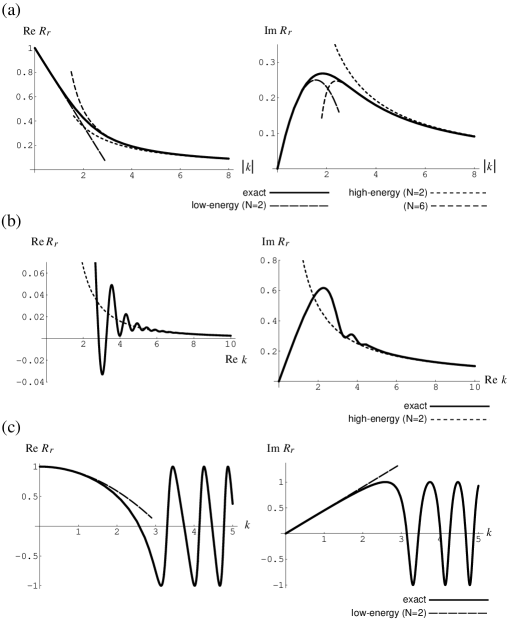
Figure 1: The real and imaginary parts of $R_{r}(x_{0},-\infty;k)$ for the potential $V(x)=x^{2}$ (example 2), where $x_{0}=-2$. They are plotted along three different lines in the complex $k$ plane: (a) $\arg k=\pi/4$;   (b) ${\rm Im}\,k=1/2$;   (c) ${\rm Im}\,k=0$.   In (a) and (b), the abscissa is $|k|$ and ${\rm Re}\,k$, respectively. Solid lines: the exact $R_{r}$ (equation (1.6adtlosd));  broken lines: the low-energy expansion (1.6adtlosg) up to order $k^{2}$; dashed lines: the high-energy expansion (1.6adtlosf) up to order $1/k^{N}$ ($N=2$ and $6$).

The series (1.6adtlosf) is divergent in this case. This asymptotic expression also holds in the case where $|k|\to\infty$ with fixed ${\rm Im}\,k>0$ (figure 1(b)). However, (1.6adtlosf) does not hold when ${\rm Im}\,k=0$. In that case the exact $R_{r}(k)$ oscillates and does not tend to zero as $|k|\to\infty$ (figure 1(c)).

The coefficients of the low-energy expansion of $R_{r}$ for this potential are also obtained from (1.6adtlos). We have $[\hbox{$-$}]_{-\infty}^{x}=\int_{-\infty}^{x}e^{-z^{2}}dz=(\sqrt{\pi}/2){\rm erfc\,}(-x)$, where ${\rm erfc\,}z$ is the Gauss error function. Substituting this into (1.6adtlos), we obtain

$$R_{r}=1+\sqrt{\pi}e^{x^{2}}{\rm erfc}\,(-x)ik+\frac{\pi}{2}e^{2x^{2}}[{\rm erfc}\,(-x)]^{2}(ik)^{2}+\cdots.$$ (1.6adtlosg)

(See figure 1.) The $R_{r}(k)$ given by (1.6adtlosd) has poles in the lower half plane. The series (1.6adtlosg) is convergent if $|k|$ is smaller than the distance from the origin to the nearest pole.

Example 3 :  $V(x)=e^{-x},\quad f(x)=\frac{1}{2}e^{-x}.$

This is an exponential potential, which tends to infinity as $x\to-\infty$ more rapidly than the previous examples. The exact $R_{r}$ has the form

$$R_{r}(x,-\infty;k)=i\frac{J_{-\nu}(-ie^{-x}/2)-ie^{-k\pi}J_{\nu}(-ie^{-x}/2)}{J_{1-\nu}(-ie^{-x}/2)+ie^{-k\pi}J_{\nu-1}(-ie^{-x}/2)},\qquad\nu\equiv ik+\frac{1}{2},$$ (1.6adtlosh)

where $J_{\alpha}(z)$ is the Bessel function. The high-energy expression (1.6adtlosp) now reads

$$R_{r}=-\frac{e^{-x}}{4ik}+\frac{e^{-x}}{2(2ik)^{2}}-\frac{4e^{-x}-e^{-3x}}{8(2ik)^{3}}+\frac{4e^{-x}-5e^{-3x}}{8(2ik)^{4}}+\cdots,$$ (1.6adtlosi)

As $|k|\to\infty$ with $\arg k$ fixed in the region $0<\arg k<\pi$, the $R_{r}$ given by (1.6adtlosh) has the asymptotic form (1.6adtlosi). However, this expression does not hold when ${\rm Im}\,k$ is kept fixed.

Using (1.6adtlos) we obtain the low-energy expansion for this potential as

$$R_{r}=1-2\exp(e^{-x}){\rm Ei}\,(-e^{-x})ik+2\exp(2e^{-x})[{\rm Ei}\,(-e^{-x})]^{2}(ik)^{2}+\cdots,$$ (1.6adtlosj)

where ${\rm Ei}\,(z)=-\int_{-z}^{\infty}(1/t)e^{-t}dt$ is the exponential integral function.

Example 4 :  $V(x)=e^{x},\quad f(x)=-\frac{1}{2}e^{x}.$

This potential falls off rapidly as $x\to-\infty$. The exact $R_{r}$ for this $V(x)$ is

$$R_{r}(x,-\infty;k)=-i\frac{J_{1-\nu}(-ie^{x}/2)}{J_{-\nu}(-ie^{x}/2)},\qquad\nu\equiv ik+\frac{1}{2}.$$ (1.6adtlosk)

From (1.6adtlosp) and (1.6adtlosl) we have

$$R_{r}=\frac{e^{x}}{4ik}+\frac{e^{x}}{2(2ik)^{2}}+\frac{4e^{x}-e^{3x}}{8(2ik)^{3}}+\frac{4e^{x}-5e^{3x}}{8(2ik)^{4}}+\cdots.$$ (1.6adtlosl)

This is the correct asymptotic expansion of (1.6adtlosk). Unlike the previous example, this expansion is valid even when ${\rm Im}\,k=0$. (See figure 2(a).)

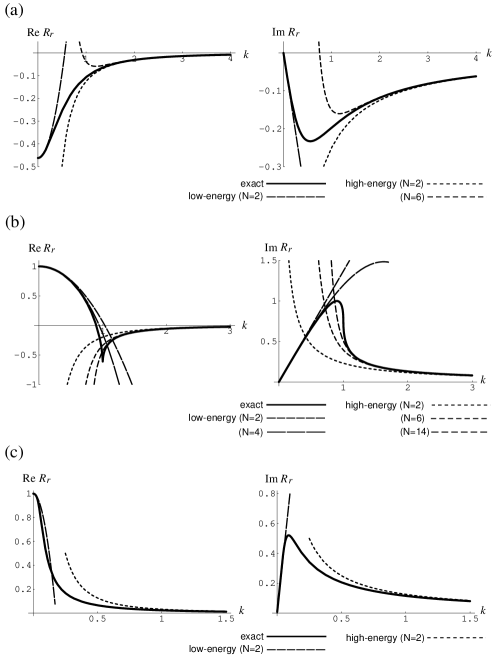
Figure 2: The real and imaginary parts of $R_{r}(x_{0},-\infty;k)$ as functions of real $k$. (a)  (example 4)  $V(x)=e^{-x}$; $x_{0}=0$. Solid lines: the exact $R_{r}$ (equation (1.6adtlosk)); broken lines: the low-energy expansion (7) up to order $k^{2}$; dashed lines: the high-energy expansion (1.6adtlosl) up to order $1/k^{N}$ ($N=2$ and $6$). (Since $k$ is real, “$N=2$” and “$N=6$” are, respectively, in effect $N=1$ and $N=5$ for ${\rm Im}\,R_{r}$.) (b)  (example 5)  $V(x)=2\log\cosh x$; $x_{0}=-1/2$. Solid lines: the exact $R_{r}$ (equation (1.6adtlosn));  broken lines: the low-energy expansion (1.6adtlosp) up to order $k^{N}$ ($N=2$ and $4$); dashed lines: the high-energy expansion (1.6adtloso) up to order $1/k^{N}$ ($N=2$, $6$, and $14$). Note that the exact $R_{r}$ is singular at $k=1$. (c)  (example 6)  $V(x)=\sqrt{-x}$; $x_{0}=-1$. Solid lines: the exact $R_{r}$ (equation (1.6adtlosq)); broken lines: the low-energy expansion (1.6adtloss) up to order $k^{2}$; dashed lines: the high-energy expansion (1.6adtlosr) up to order $1/k^{2}$.

The low-energy expansion for this potential is correctly given by (1.6adtlor) with (1.6adtlos):

$$R_{r}=-\tanh\frac{e^{x}}{2}-\left({\rm sech\,}\frac{e^{x}}{2}\right)^{2}\,{\rm Shi\,}(e^{x})\,ik$$

$$-2\left({\rm sech\,}\frac{e^{x}}{2}\right)^{3}\left[\int_{0}^{e^{x}}\frac{\cosh(y-{\textstyle\frac{1}{2}}e^{x})}{y}{\rm Shi\,}(y)\,dy\right](ik)^{2}+\cdots,$$ (1.6adtlosm)

where ${\rm Shi\,}(z)=\int_{0}^{z}(1/t)\sinh t\,dt$ is the hyperbolic sine integral function (figure 2(a)). The radius of convergence of (7) is larger than $1/2$, and it approaches $1/2$ as $x\to-\infty$.

Example 5 :  $V(x)=2\log\cosh x,\quad f(x)=-\tanh x.$

This is another example of a potential that grows linearly as $x\to-\infty$. The exact form of the reflection coefficient is expressed in terms of the hypergeometric function $F(\alpha,\beta,\gamma;z)=\frac{\Gamma(\gamma)}{\Gamma(\alpha)\Gamma(\beta)}\sum_{n=0}^{\infty}\frac{\Gamma(\alpha+n)\Gamma(\beta+n)}{\Gamma(\gamma+n)}\frac{1}{n!}z^{n}$. We define

$$\eta(x,k) \equiv F\left(\alpha,\beta,{\textstyle\frac{1}{2}};-\sinh^{2}x\right)+2\frac{\Gamma\left(\frac{1}{2}+\alpha\right)\Gamma(1-\beta)}{\Gamma(\alpha)\Gamma\left(\frac{1}{2}-\beta\right)}\sinh xF\left(\alpha+{\textstyle\frac{1}{2}},\beta+{\textstyle\frac{1}{2}},{\textstyle\frac{3}{2}};-\sinh^{2}x\right)$$

with $\alpha\equiv\frac{1}{2}[-1-ik\sqrt{1-(1/k)^{2}}]$, $\beta\equiv\frac{1}{2}[-1+ik\sqrt{1-(1/k)^{2}}].$ Then we have

$$R_{r}(x,-\infty;k)=\frac{ik\eta(x,k)+\eta^{\prime}(x,k)}{ik\eta(x,k)-\eta^{\prime}(x,k)},$$ (1.6adtlosn)

where $\eta^{\prime}=\partial\eta/\partial x$. The high-energy expansion (1.6adtlosp) now takes the form

$$R_{r} =\frac{\tanh x}{2ik}+\frac{({\rm sech\,}x)^{2}}{(2ik)^{2}}-\frac{(3+\cosh 2x)({\rm sech\,}x)^{2}\tanh x}{2(2ik)^{3}}-\frac{(3+\cosh 2x)({\rm sech\,}x)^{4}}{2(2ik)^{4}}$$ (1.6adtloso)

$$\qquad+\frac{(11+8\cosh 2x+\cosh 4x)({\rm sech\,}x)^{4}\tanh x}{4(2ik)^{5}}+\cdots.$$

As shown in figure 2(b), this is the correct large-$|k|$ expansion of (1.6adtlosn) for ${\rm Im}\,k\geq 0$. As in example 1, the series (1.6adtloso) is convergent for $|k|>1$.

Calculating (1.6adtlos) for this potential, we obtain the low-energy expansion

$$R_{r} =1+2(\cosh x)e^{x}ik+2(\cosh x)^{2}e^{2x}(ik)^{2}+\left[2(\cosh x)^{3}e^{3x}-(\cosh x)^{2}e^{2x}\right](ik)^{3}$$ (1.6adtlosp)

$$\qquad+\left[2(\cosh x)^{4}e^{4x}-4(\cosh x)^{4}e^{2x}+2(\cosh x)^{3}e^{x}\right](ik)^{4}+\cdots.$$

This is the correct small-$|k|$ expansion of (1.6adtlosn), as can be seen from figure 2(b).

Example 6 :  $\displaystyle V(x)=\sqrt{-x},\quad f(x)=\frac{1}{4}\frac{1}{\sqrt{-x}}.$  ($x_{\rm max}=0$.)

In this example, $V(x)$ slowly tends to infinity as $x\to-\infty$, while $f(x)$ slowly converges to zero. The exact $R_{r}(x,-\infty)$ $(x<0)$ has the form

$$R_{r}(x,-\infty;k)=\frac{b(x,k)}{a(x,k)},$$ (1.6adtlosq)

$$a(x,k)\equiv 2\Gamma\left(\alpha+1\right)F\left(\alpha,{\textstyle\frac{1}{2}};2ikx\right)-\frac{1}{4}\left(\frac{i}{2k}\right)^{1/2}\,\Gamma\left(\alpha+{\textstyle\frac{1}{2}}\right)\sqrt{-x}\,F\left(\alpha+{\textstyle\frac{1}{2}},{\textstyle\frac{3}{2}};2ikx\right),$$

$$b(x,k)\equiv-\Gamma\left(\alpha+1\right)\sqrt{-x}\,F\left(\alpha+1,{\textstyle\frac{3}{2}};2ikx\right)+\frac{1}{2}\left(\frac{i}{2k}\right)^{1/2}\Gamma\left(\alpha+{\textstyle\frac{1}{2}}\right)F\left(\alpha+{\textstyle\frac{1}{2}},{\textstyle\frac{1}{2}};2ikx\right),$$

where $\alpha\equiv i/(32k)$. Expression (1.6adtlosp) now reads

$$R_{r}=-\frac{(-x)^{-1/2}}{8ik}-\frac{(-x)^{-3/2}}{8(2ik)^{2}}-\frac{(x+12)(-x)^{-5/2}}{64(2ik)^{3}}-\frac{(5x+60)(-x)^{-7/2}}{128(2ik)^{4}}+\cdots.$$ (1.6adtlosr)

This is the high-energy asymptotic expansion of (1.6adtlosq) which is valid as long as $x<0$. This expansion holds even for real $k$. (See figure 2(c).)

The low-energy expansion is obtained from (1.6adtlos) as

$$R_{r} =1+4\left(1+\sqrt{-x}\,\right)ik+8\left(1+\sqrt{-x}\,\right)^{2}(ik)^{2}-32\left(5+4\sqrt{-x}-x\right)(ik)^{3}$$ (1.6adtloss)

$$\qquad+32\left(-21-40\sqrt{-x}+26x+8x\sqrt{-x}-x^{2}\right)(ik)^{4}+\cdots.$$

This is the correct asymptotic expansion of (1.6adtlosq) (figure 2(c)). Unlike examples 1–5, this series is divergent; the $R_{r}(k)$ given by (1.6adtlosq) is essentially singular at $k=0$.

Example 7 :  $\displaystyle V(x)=\alpha\log(-x),\quad f(x)=-\frac{\alpha}{2x}.$  ($x_{\rm max}=0$.)

Here $\alpha$ is a positive constant. This potential tends to infinity as $x\to-\infty$ even more slowly than the previous one. The exact $R_{r}(x,-\infty)$ $(x<0)$ is expressed in terms of the Bessel function as

$$R_{r}(x,-\infty;k)=\frac{[J_{\nu}(-kx)+iJ_{\nu-1}(-kx)]-ie^{i\alpha\pi/2}[J_{-\nu}(-kx)-iJ_{1-\nu}(-kx)]}{[J_{\nu}(-kx)-iJ_{\nu-1}(-kx)]-ie^{i\alpha\pi/2}[J_{-\nu}(-kx)+iJ_{1-\nu}(-kx)]},$$ (1.6adtlost)

where $\nu\equiv(1+\alpha)/2$. From (1.6adtlosp) and (1.6adtlosl) we have

$$R_{r}=\frac{\alpha}{4xik}-\frac{\alpha}{2x^{2}(2ik)^{2}}-\frac{\alpha^{3}-8\alpha}{8x^{3}(2ik)^{3}}+\frac{5\alpha^{3}-24\alpha}{8x^{4}(2ik)^{4}}+\cdots.$$ (1.6adtlosu)

We can check that this high-energy expansion is correct even when ${\rm Im}\,k=0$.

On the other hand, the low-energy expression (1.6adtlor) for this $V(x)$ reads

$$R_{r}=1+2(-x)^{\alpha}ik\int_{-\infty}^{x}\frac{1}{(-z)^{\alpha}}\,dz+\cdots,$$ (1.6adtlosv)

but the integral on the right-hand side is divergent if $\alpha\leq 1$. From the exact expression (1.6adtlost) we can see that the correct asymptotic form for $\alpha\leq 1$ is

$$R_{r}=1-2^{1-\alpha}\frac{\Gamma\left(\frac{1-\alpha}{2}\right)}{\Gamma\left(\frac{1+\alpha}{2}\right)}(-x)^{\alpha}k^{\alpha}+\cdots,$$ (1.6adtlosw)

which includes a fractional power of $k$. If $\alpha>1$, then (1.6adtlosv) is correct to order $k$, but the expansion in integral powers of $k$ fails at some higher order.

Example 8 : Potential with a singularity.

As an example of a potential that has a singularity on the real axis, let us consider

$$V(x)=\cases{e^{-x}&$(x<0)$\\ 1-x&$(x>0)$},\qquad f(x)=\cases{{\textstyle\frac{1}{2}}e^{-x}&$(x<0)$\\ {\textstyle\frac{1}{2}}&$(x>0)$}.$$ (1.6adtlosx)

In this case, $f(x)$ is continuous and piecewise differentiable. The derivative of $f(x)$ has a jump at $x=0$. The exact $R_{r}(x,-\infty)$ for $x>0$ has the form

$$R_{r}(x,-\infty;k)=\frac{-ik\left(A-2\right)B+1+\left[-ik\left(A+2\right)B-1\right]e^{ikAx}}{-ik\left(A+2\right)+B+\left[-ik\left(A-2\right)-B\right]e^{ikAx}},$$ (1.6adtlosy)

$$A\equiv\sqrt{4-(1/k^{2})},\qquad B\equiv i\frac{J_{-\nu}(-i/2)-ie^{-k\pi/2}J_{\nu}(-i/2)}{J_{1-\nu}(-i/2)+ie^{-k\pi/2}J_{\nu-1}(-i/2)},\qquad\nu\equiv ik+\frac{1}{2}.$$ (1.6adtlosz)

(This $B$ is the value of (1.6adtlosh) at $x=0$.) Now (1.6adtlosp) and (1.6adtlosl) yield the expansion

$$R_{r}=-\frac{1}{4ik}+\frac{1}{(4ik)^{3}}-\frac{2}{(4ik)^{5}}+\frac{5}{(4ik)^{7}}+\cdots.$$ (1.6adtlosaa)

If the limit $|k|\to\infty$ is taken with $0<\arg k<\pi$, then the $e^{ikAx}$ in (1.6adtlosy) falls off faster than any power of $1/k$, and we can show that (1.6adtlosaa) is the correct asymptotic expansion. (See the comments at the end of section 6.) If ${\rm Im}\,k=0$, then the $e^{ikAx}$ cannot be neglected. In this example, (5.15) does not hold for any $N$ when ${\rm Im}\,k=0$. The low-energy expression (1.6adtlor) is valid irrespective of the presence of the singularity.

8 Summary

The generalized reflection coefficient for the semi-infinite interval, $\bar{R}_{r}(x,-\infty;\xi)$, is expressed in the form of (1.6ado) in terms of the operators ${\cal A}$ and ${\cal B}$ defined by (1.6ada) and (1.6adb). Using the operator equations (1.6adta) and (1.6adtb), with ${\cal L}$ defined by (1.6ads), we can derive expansions of $\bar{R}_{r}$ in powers of $k$ and $1/k$, together with the remainder terms (equations (1.6adtc) and (1.6adtlosa)). For either the low-energy or the high-energy expansion, the remainder term is expressed in terms of the inverse operator $({\cal A}-2ik{\cal B})^{-1}$, and, according to (1.6adg), it can be written as integrals involving the scattering coefficients ((1.6adtlm) and (1.6adtlosi)). By using the asymptotic forms of the scattering coefficients given in appendix A, we can study the behavior of the remainder term as $k\to 0$ or $|k|\to\infty$, and investigate whether the expansion is asymptotic or not. The results are roughly summarized in figure 3. For the high-energy expansion, conditions concerning differentiability of the potential must also be taken into account, as explained in section 6.

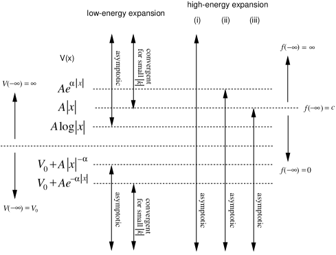
Figure 3: Domains of validity of the low-energy expansion (1.6adtlor) and the high-energy expansion (1.6adtlosp), where the limit $|k|\to\infty$ is taken with: (i) fixed $\arg k$ ($0<\arg k<\pi$); (ii) fixed ${\rm Im}\,k>0$; (iii) ${\rm Im}\,k=0$.

(The problem of whether the high-energy expansion is convergent or not is beyond the scope of this paper.)

Appendix A Asymptotic behavior of $\bar{\tau}(x,y)$ and $\bar{R}_{l}(x,y)$ as $y\to-\infty$

Here we summarize the asymptotic forms of $\bar{\tau}(x,y;\xi;k)$ and $\bar{R}_{l}(x,y;\xi;k)$ as $y\to-\infty$ with fixed $x$, $\xi$, and $k$ (${\rm Im}\,k\geq 0$). (The derivation is omitted for space limitations.)

(i) $f(-\infty)=\pm\infty$

In this case the asymptotic form of $\bar{\tau}(x,y)$ as $y\to-\infty$ is

$$\bar{\tau}(x,y;\xi;k)=C(x,\xi,k)\exp\left[-\frac{1}{2}|V(y)|+\eta(y,k)\right][1+o(1)],$$ (1.6adtlosa)

where $\eta(y,k)=o(|y|)$ $(y\to-\infty)$. If $1/f(y)=O(1/|y|^{1+\epsilon})$ with some positive number $\epsilon$, then $\eta(y,k)=O(1)$. In that case we may let $\eta(-\infty,k)$ be absorbed into the $y$-independent quantity $C$, and redefine $\eta$ to be identically zero. The $\bar{R}_{l}$ behaves as

$$\bar{R}_{l}(x,y;\xi;k)=\mp 1-\frac{ik}{f(y)}[1+o(1)],$$ (1.6adtlosb)

where the $\mp 1$ on the right-hand side corresponds to $f(-\infty)=\pm\infty$, respectively.

(ii) $f(-\infty)=c\quad(c\neq 0,\pm\infty)$

When ${\rm Re\,}\sqrt{c^{2}-k^{2}}>0$ (i.e., ${\rm Im\,}k>0$ or ${\rm Im\,}k=0$, $c^{2}>k^{2}$), we have, as $y\to-\infty$,

$$\bar{\tau}(x,y;\xi;k)=C(x,\xi,k)\exp\left[\sqrt{c^{2}-k^{2}}\,y+\eta(y,k)\right][1+o(1)],$$ (1.6adtlosc)

$$\bar{R}_{l}(x,y;\xi;k)=-\frac{1}{c}\left(ik+\sqrt{c^{2}-k^{2}}\,\right)+o(1),$$ (1.6adtlosd)

where $\eta(y,k)=o(|y|)$. If $f(y)=c+O(1/|y|^{1+\epsilon})$ with some positive $\epsilon$, then $\eta(y,k)=O(1)$, and so we may take $\eta$ to be zero.

When $k$ is real and $k^{2}\geq c^{2}$, equations (1.6adtlosc) and (1.6adtlosd) do not hold. When evaluating an integral like (1.6adg) in such cases, we need to add an imaginary part $i\epsilon$ ($\epsilon>0$) to $k$, and let $\epsilon\to 0$ afterwards. This is because $\bar{R}_{r}(k)$ has branch cuts along the real axis.

(iii) $f(-\infty)=0$

In this case we have, as $y\to-\infty$,

$$\bar{\tau}(x,y;\xi;k)=C(x,\xi,k)\exp[-iky+i\theta(y,k)][1+o(1)],\quad k\neq 0,$$ (1.6adtlose)

where $\theta(y,k)=o(|y|)$. If $f^{2}(y)=O(1/|y|^{1+\epsilon})$, then we may let $\theta=0$. If ${\rm Im}\,k>0$, then

$$\bar{R}_{l}(x,y;\xi;k)=o(1).$$ (1.6adtlosf)

If ${\rm Im}\,k=0$, then $\bar{R}_{l}(x,y)$ does not vanish but oscillates as $y\to-\infty$:

$$\bar{R}_{l}(x,y;\xi;k)=D(x,\xi,k)\exp\left[-2iky+2i\theta(y,k)\right]+o(1),\quad k\neq 0,$$ (1.6adtlosg)

where $D(x,\xi,k)$ is another quantity independent of $y$. The $\theta(y,k)$ in (1.6adtlosg), which is the same one as in (1.6adtlose), is a real quantity when $k$ is real.

Appendix B Proof of (1.6adh) with (1.6adg)

We are assuming that $g(x,\xi)$ is an analytic function of $\xi$ in $-1<\xi<1$, as mentioned at the beginning of section 5. So we may expand $g/(1-\xi^{2})$ in powers of $\xi$ and write

$$g(x,\xi)\equiv(1-\xi^{2})\sum_{n=0}^{\infty}\xi^{n}h_{n}(x).$$ (1.6adtlosa)

We consider each term of (1.6adtlosa) separately. Calculating with (1.6ada) and (1.6adb), we have

$$({\cal A}-2ik{\cal B})(1-\xi^{2})\xi^{n}h_{n}(x)$$

$$\qquad=(1-\xi^{2})\Biggl{\{}\xi^{n}\frac{dh_{n}(x)}{dx}+\left[n\xi^{n-1}-(n+2)\xi^{n+1}\right]f(x)h_{n}(x)-2(n+1)ik\xi^{n}h_{n}(x)\Biggr{\}}.$$

Let us apply $({\cal A}-2ik{\cal B})^{-1}$ given by (1.6adg) to the first term on the right-hand side:

$$\frac{1}{{\cal A}-2ik{\cal B}}(1-\xi^{2})\xi^{n}\frac{dh_{n}(x)}{dx}=\int_{-\infty}^{x}\bar{\tau}^{2}(x,z;\xi)\bar{R}_{l}^{n}(x,z;\xi)\frac{dh_{n}(z)}{dz}\,dz$$

$$\qquad=\tau^{2}(x,z;\xi)\bar{R}_{l}^{n}(x,z;\xi)h_{n}(z)\Big{|}_{z=-\infty}^{z=x}-\int_{-\infty}^{x}\frac{\partial}{\partial z}\left[\bar{\tau}^{2}(x,z;\xi)\bar{R}_{l}^{n}(x,z;\xi)\right]h_{n}(z)\,dz.$$ (1.6adtlosc)

It can be shown that $\tau$ and $R_{l}$ satisfy the differential equations [11]

$$\frac{\partial}{\partial z}\bar{\tau}(x,z)=-ik\bar{\tau}(x,z)-f(z)\bar{\tau}(x,z)\bar{R}_{l}(x,z),$$ (1.6adtlosd)

$$\frac{\partial}{\partial z}\bar{R}_{l}(x,z)=-2ik\bar{R}_{l}(x,z)+f(z)\left[1-\bar{R}_{l}^{2}(x,z)\right].$$ (1.6adtlose)

Using (1.6adtlosd) and (1.6adtlose), we can rewrite the integral in the last expression of (B) as

$$\int_{-\infty}^{x}\frac{\partial}{\partial z}\left[\bar{\tau}^{2}(x,z;\xi)\bar{R}_{l}^{n}(x,z;\xi)\right]h_{n}(z)\,dz$$

$$\qquad=\int_{-\infty}^{x}\bar{\tau}^{2}\left[n\bar{R}_{l}^{n-1}-(n+2)\bar{R}_{l}^{n+1}\right]fh_{n}\,dz-2(n+1)ik\int_{-\infty}^{x}\bar{\tau}^{2}\bar{R}_{l}^{n}h_{n}\,dz$$

$$\qquad=\frac{1}{{\cal A}-2ik{\cal B}}(1-\xi^{2})\left\{\left[n\xi^{n-1}-(n+2)\xi^{n+1}\right]f(x)h_{n}(x)-2(n+1)ik\xi^{n}h_{n}(x)\right\}.$$

From (B), (B), and (B) we have

$$\frac{1}{{\cal A}-2ik{\cal B}}({\cal A}-2ik{\cal B})(1-\xi^{2})\xi^{n}h_{n}(x)=\bar{\tau}^{2}(x,z;\xi)\bar{R}_{l}^{n}(x,z;\xi)h_{n}(z)\Big{|}_{z=-\infty}^{z=x}.$$ (1.6adtlosg)

Taking the sum over $n$ and using definition (1.6adtlosa) gives

$$\frac{1}{{\cal A}-2ik{\cal B}}({\cal A}-2ik{\cal B})g(x,\xi)=\left.\frac{\bar{\tau}^{2}(x,z;\xi)}{1-\bar{R}_{l}^{2}(x,z;\xi)}\,g(z,\bar{R}_{l}(x,z;\xi))\right|_{z=-\infty}^{z=x}.$$ (1.6adtlosh)

If (1.6adf) is satisfied, then we can easily see, by using (1.6ab), that the right-hand side of (1.6adtlosh) is equal to $g(x,\xi)$. Thus $({\cal A}-2ik{\cal B})^{-1}({\cal A}-2ik{\cal B})g=g$ holds.

Appendix C Proof of (1.6adm)

With $g=\bar{R}_{r}+\xi$, the expression to the right of the limit symbol in (1.6adf) reads

$$\frac{\bar{\tau}^{2}(x,z;\xi)}{1-\bar{R}_{l}^{2}(x,z;\xi)}\left[\frac{R_{r}(z,-\infty)-\bar{R}_{l}(x,z;\xi)}{1-R_{r}(z,-\infty)\bar{R}_{l}(x,z;\xi)}+\bar{R}_{l}(x,z;\xi)\right]=\frac{\bar{\tau}^{2}(x,z;\xi)R_{r}(z,-\infty)}{1-R_{r}(z,-\infty)\bar{R}_{l}(x,z;\xi)}.$$

From (1.6adtlosa), (1.6adtlosc), and (1.6adtlose), we can see that $\lim_{z\to-\infty}\bar{\tau}(x,z)=0$ if $f(-\infty)=\pm\infty$ or ${\rm Im}\,k>0$. On the other hand, if $f(-\infty)=0$ then $\lim_{z\to-\infty}R_{r}(z,-\infty)=0$. Therefore, the right-hand side vanishes in the limit $z\to-\infty$ for all $k$ with ${\rm Im}\,k\geq 0$, except in the case $f(-\infty)=c\,(\neq 0,\pm\infty)$ with ${\rm Im}\,k=0$. (For this exceptional case, see the comment in (ii) of appendix A.)

Appendix D Explicit forms of (4) and the remainder terms

The right-hand sides of (1.6adtla) and (1.6adtlb) can be explicitly calculated. The result is

$$C^{\pm}_{s_{1},s_{2},\ldots,s_{n-1}}(W)=c^{\pm}_{s_{1},\ldots,s_{n-1}}\exp\biggl{[}\Bigl{(}\pm 1-\sum_{i=1}^{n-1}s_{i}\Bigr{)}W\biggr{]},$$ (1.6adtlosa)

$$c^{\pm}_{s_{1},\ldots,s_{n-1}}\equiv\pm 2\prod_{j=1}^{n-1}\biggl{[}\mp s_{j}\Bigl{(}1\mp\sum_{k=1}^{j}s_{k}\Bigr{)}\biggr{]}.$$ (1.6adtlosb)

The expression for $D_{s_{1},s_{2},\ldots,s_{n-1}}(W)$ can be written in the form

$$D_{s_{1},s_{2},\ldots,s_{n-1}}(W)={\rm sech}^{n+1}[(V_{0}-W)/2]\sum_{m=-n+1}^{n-1}d_{s_{1},\ldots,s_{n-1};m}\exp\left({\textstyle\frac{1}{2}}mW\right).$$ (1.6adtlosc)

where $d_{s_{1},\ldots,s_{n-1};m}$ are constants. (We omit writing out the expressions for them.)

Substituting (4) (with (1.6adtlosa) and (1.6adtlosc)) into (1.6adtln) and (1.6adtlm), we may write

$$\bar{\rho}_{n} =(ik)^{n+1}\sum_{\{s_{1},\ldots,s_{n}\}}\int_{-\infty}^{x}\frac{\bar{\tau}^{2}(x,z)}{1-\bar{R}_{l}^{2}(x,z)}\,P^{+}_{s_{1},\ldots,s_{n}}(x,z)$$ (1.6adtlosd)

$$\qquad\qquad\qquad\qquad\times[-1,s_{1},s_{2},\ldots,s_{n-1}]_{-\infty}^{z}e^{s_{n}V(z)}\,dz,\qquad V(-\infty)=+\infty,$$

$$=(ik)^{n+1}\sum_{\{s_{1},\ldots,s_{n}\}}\int_{-\infty}^{x}\frac{\bar{\tau}^{2}(x,z)}{1-\bar{R}_{l}^{2}(x,z)}\,P^{-}_{s_{1},\ldots,s_{n}}(x,z)$$

$$\qquad\qquad\qquad\qquad\times[+1,s_{1},s_{2},\ldots,s_{n-1}]_{-\infty}^{z}e^{s_{n}V(z)}\,dz,\qquad V(-\infty)=-\infty,$$

$$=(ik)^{n+1}\sum_{\{s_{1},\ldots,s_{n}\}}\int_{-\infty}^{x}\frac{\bar{\tau}^{2}(x,z)}{1-\bar{R}_{l}^{2}(x,z)}\,Q_{s_{1},\ldots,s_{n}}(x,z)$$

$$\qquad\qquad\qquad\qquad\times(\pm,s_{1},s_{2},\ldots,s_{n-1}]_{-\infty}^{z}e^{s_{n}V(z)}\,dz,\qquad V(-\infty)=V_{0},$$

where

$$P^{\pm}_{s_{1},s_{2},\ldots,s_{n}}(x,z)=c^{\pm}_{s_{1},\ldots,s_{n}}\left[\frac{1+\bar{R}_{l}(x,z)}{1-\bar{R}_{l}(x,z)}\right]^{\pm 1-\sum_{i=1}^{n}s_{i}}\exp\biggl{[}\Bigl{(}\pm 1-\sum_{i=1}^{n}s_{i}\Bigr{)}V(z)\biggr{]},$$ (1.6adtlose)

$$Q_{s_{1},s_{2},\ldots,s_{n}}(x,z) =\frac{\left[1-\bar{R}_{l}^{2}(x,z)\right]^{(n/2)+1}}{\left\{\cosh{\textstyle\frac{1}{2}}[V(z)-V_{0}]+\bar{R}_{l}(x,z)\sinh{\textstyle\frac{1}{2}}[V(z)-V_{0}]\right\}^{n+2}}$$ (1.6adtlosf)

$$\qquad\qquad\times\sum_{m=-n}^{n}d_{s_{1},\ldots,s_{n};m}\left[\frac{1+\bar{R}_{l}(x,z)}{1-\bar{R}_{l}(x,z)}\right]^{m/2}\exp\left[{\textstyle\frac{1}{2}}mV(z)\right].$$

Appendix E Finiteness of $\bar{\rho}_{N}$ and $\bar{\delta}_{N}$

The domain of $({\cal A}-2ik{\cal B})^{-1}$ is the range of ${\cal A}-2ik{\cal B}$ with its domain restricted to $\Omega^{[V]}_{k}$. It is obvious that ${\cal A}\,\bar{r}_{N+1}$ belongs to the domain of $({\cal A}-2ik{\cal B})^{-1}$ if $\bar{r}_{0}+\xi$ and $\bar{r}_{1},\bar{r}_{2},\ldots.\bar{r}_{N}$ all belong to $\Omega^{[V]}_{k}$. Namely, if $\bar{r}_{0}+\xi$ and $\bar{r}_{n}$ ($1\leq n\leq N$) satisfy condition (1.6adf), then (1.6adte) makes sense and is finite. Using the asymptotic forms of $\bar{\tau}$ and $\bar{R}_{l}$ given in appendix A, and the expressions for $\bar{r}_{n}$ given by (4) with (1.6adtlosa) and (1.6adtlosc), we can show that these conditions are satisfied as long as the $\bar{r}_{n}$ are finite. (When $k$ is a nonzero real number, we need to be careful in the following two cases: the case $f(-\infty)=c$ with $k^{2}>c^{2}\neq 0$, and the case where $f(-\infty)=0$ and $V(-\infty)=\pm\infty$. In these cases, the value of the integral (1.6adtlm) is indeterminate. So we need to replace $k$ by $k+i\epsilon$ with positive infinitesimal $\epsilon$, and let $\epsilon\to 0$ after evaluating the integral. Then the integral takas a definite value, and expression (1.6adtc) is well-defined.)

Similarly, ${\cal B}\,\bar{c}_{N+1}$ lies in the domain of $({\cal A}-2ik{\cal B})^{-1}$ if $\bar{c}_{1},\bar{c}_{2},\ldots,\bar{c}_{N}$ belong to $\Omega^{[V]}_{k}$. It is easy to see that this condition is satisfied as long as $\bar{c}_{1}(x,\xi),\ldots,\bar{c}_{N}(x,\xi)$ are continuous and piecewise differentiable with respect to $x$

Appendix F Verification of (1.6adtlosu)

Here we study the cases $V(-\infty)=+\infty$ and $V(-\infty)=V_{0}$. The former is divided into two subcases, $f(-\infty)\neq 0$ and $f(-\infty)=0$. We omit the case $V(-\infty)=-\infty$, which is essentially the same as the case $V(-\infty)=+\infty$.

(i)-A  $V(-\infty)=+\infty$,  $f(-\infty)\neq 0$

The first equation of (1.6adtlosd) has the form

$$\bar{\rho}_{n}=(ik)^{n+1}\int_{-\infty}^{x}B_{n}(z,k)\bar{\tau}^{2}(x,z;k)\,dz.$$ (1.6adtlosa)

(In this appendix, we regard $x$ and $\xi$ as fixed constants.) Using (1.6adtlosb), (1.6adtlose), and (1.6adtlosb), we can show that $B_{n}(z,k)$ tends to a finite value as $z\to-\infty$.

When $f(-\infty)=+\infty$ or $f(-\infty)=c\neq 0$, the behavior or $\bar{\tau}(x,z)$ as $z\to-\infty$ is given by (1.6adtlosa) or (1.6adtlosc). In either case there exist real constants $C_{1}$, $C_{2}$, and $k_{1}$ such that $|\bar{\tau}^{2}(x,z;k)|\leq C_{1}e^{-V(z)+C_{2}z}$ for $z<x$ and $|k|<k_{1}$. Using this, we can easily show

$$\lim_{k\to 0}\int_{-\infty}^{x}B_{n}(z,k)\bar{\tau}^{2}(x,z;k)\,dz=\int_{-\infty}^{x}\lim_{k\to 0}B_{n}(z,k)\bar{\tau}^{2}(x,z;k)\,dz,$$ (1.6adtlosb)

which is equivalent to the second equality of (1.6adtlosu).

(i)-B  $V(-\infty)=+\infty$,  $f(-\infty)=0$

If $V(x)$ tends to infinity more slowly than $|x|$ as $x\to-\infty$, the asymptotic behavior or $\bar{\tau}(x,z)$ is given by (1.6adtlose). The quantity $B_{n}(z,k)$ of (1.6adtlosa) becomes infinite as $z\to-\infty$ for $n\geq 1$. We can show that $B_{n}$ does not grow faster than $|z|^{n}$, i.e., $B_{n}(z,k)=o(|z|^{n})$.

Here we give only a sketchy explanation. Let $f(z)$ be monotone for $z<z_{1}$. For any $k$ satisfying $|k|<|f(z_{1})|$, there exists a value $z_{a}(k)$ $(<z_{1})$ such that $|k|=|f(z_{a})|$. As $k$ approaches zero, this $z_{a}$ tends to $-\infty$. Let $k$ be sufficiently small. Then $\bar{\tau}(x,z;k)\simeq\bar{\tau}(x,z;k=0)$ for $z\gg z_{a}$, and $\bar{\tau}(x,z;k)\simeq\bar{\tau}(x,z_{a};k=0)\exp[-ik(z-z_{a})+\cdots]$ for $z\ll z_{a}$. Using $B_{n}(z,k)=o(|z|^{n})$, we have the estimate

$$\lim_{k\to 0}\left|\int_{-\infty}^{z_{a}(k)}B_{n}(z,k)\bar{\tau}^{2}(x,z;k)\,dz\right|<C\,\lim_{k\to 0}\frac{e^{-2V(z_{a}(k))}}{k^{n+1}}=C\lim_{z_{a}\to-\infty}\frac{e^{-2V(z_{a})}}{f^{n+1}(z_{a})},$$ (1.6adtlosc)

where $C$ is a constant. The last expression of (1.6adtlosc) vanishes if $V(z)$ tends to infinity faster than $\log|z|$ as $z\to-\infty$. Hence we can see that (1.6adtlosb) holds even in this case.

(ii)  $V(-\infty)=V_{0}\neq\infty$

Let us consider each integral in the last expression of (1.6adtlosd). From (1.6adtlose), (1.6adtlosf), and (1.6adtlosf), we can see that there exist constants $C$ and $k_{1}$ such that

$$\left|\frac{\bar{\tau}^{2}(x,z;k)}{1-\bar{R}_{l}^{2}(x,z;k)}\,Q_{s_{1},\ldots,s_{n}}(x,z;k)\right|\leq C$$ (1.6adtlosd)

for any $z<x$ and $|k|<k_{1}$. Thus, the integrand in the last expression of (1.6adtlosd) is absolutely dominated by $C(\pm,s_{1},s_{2},\ldots,s_{n-1}]_{-\infty}^{z}e^{s_{n}V(z)}$, which is a $k$-independent function of $z$. The integral of this function is $C\,(\pm,s_{1},s_{2},\ldots,s_{n-1},s_{n}]_{-\infty}^{x}$, which is finite if the potential satisfies condition (1.6adtlob). Therefore we can interchange the limit $k\to 0$ and the integral in (1.6adtlosd), and so the second equality of (1.6adtlosu) holds.

References

References

[1]
Risken H 1984 The Fokker-Planck Equation (Berlin: Springer)
[2]
Newton R G 1966 Scattering Theory of Waves and Particles
(New York: McGraw-Hill)
[3]
Deift P and Trubowitz E 1979 Commun. Pure Appl. math.32 121
[4]
Chadan K and Sabatier P C 1989 Inverse Problems in Quantum Scattering Theory 2nd ed.
(New York: Springer)
[5]
Rybkin A 2002 Bull. London Math. Soc.34 61
[6]
Rybkin A 2002 Proc. Amer. Math. Soc.130 59
[7]
Aktosun T and Klaus M 2001 Inverse Problems17 619
[8]
Aktosun T, Klaus M and van der Mee, C 2001 J. Math. Phys.42 4627
[9]
Hinton D B, Klaus M and Shaw J K 1989 Inverse Problems5 1049
[10]
Bollé D, Gesztesy F and Wilk S F J 1985 J. Oper. Theory13 3