Nature of the inhomogeneous state of the extended t-J model on a square lattice

Abstract

We carry out the variational Monte Carlo calculation to examine spatially inhomogeneous states in hole- and electron-doped cuprates. By using Gutzwiller approximation, we consider the excitations, arising from charge density, spin density and pair field, of the mean-field ground state of the $t-J$ model. It leads to the stripe patterns we have found numerically in a generalized $t-J-$type model including mass renormalization from the electron-phonon coupling. In the hole-doped side, a robust $d$-wave superconducting order results in the formation of the half-doped antiferromagnetic resonating-valence-bond (AF-RVB) stripes shown by the well-known Yamada plot. On the other hand, due to a long-range AF order in electron-doped materials, a stripe structure with the ”in-phase” magnetic domain (IPMD) is obtained in the underdoped regime instead of the AF-RVB stripe. The IPMD stripe with the largest period permitted by lattice size is stabilized near the underdoped region and it excludes the Yamada plot from electron-doped cases. Based on finite lattice size to which we can reach, the existence of IPMD stripes may imply an electronic phase separation into an electron-rich and an insulating half-filled AF long-range ordered domains in electron-doped compounds.

Since the discovery of high-temperature superconductivity in the layered cuprate materials, there have been many evidences for stripe structures in several families of the hole-doped cuprates, e.g., $La_{2-\delta}Sr_{\delta}CuO_{4}$ TranquadaNat95 ; KivelsonRMP03 . One of the many puzzles of the stripes is the doping dependence of the incommensurate magnetic peaks associated with the stripes measured by neutron-scattering experiments which obeys the so-called Yamada plot YamadaPRB98 . It represents the existence of the half-doped stripe with average of $1/2$ hole in one charge modulation period at $1/8$ hole density and below. There have been many early theoretical works attempting to explain the Yamada plot MartinsPRL00 ; WhitePRL98 ; ArrigoniPRB02 . One possible scenario for such correlation is that tendency for charges toward phase separation can lead to various structures including stripes, puddles ZaanenPRB89 ; EmeryPhysC93 , or even cluster glasses with randomly-oriented stripe domains recently observed by scanning tunneling spectroscopy (STS) KohsakaSci07 ; ParkerNat10 . Recently we have used a variational Monte Carlo (VMC) technique CPCPRB10 to successfully establish the half-doped stripes in the extended $t-J-$type Hamiltonian by including a mass-renormalization effect due to a weak electron-phonon coupling.

So far the experimental situation in electron-doped materials is much less clear ArmitageRMP10 . There are several indirect evidences for a homogeneous state in electron-doped compounds coming from measurements of neutron scattering and core-level photoemission spectra HarimaPRB01 ; MotoyamaPRL06 . Yamada et al. have reported only commensurate spin fluctuations observed by neutron scattering in the superconducting (SC) $Nd_{1.85}Ce_{0.15}CuO_{4}$ YamadaPRL03 . It is different from the incommensurate peaks observed in hole-doped cuprates which are considered as the hall mark of the ”out-of-phase” stripe domains with a $\pi$-phase-shifted staggered magnetic moment. Instead of stripes, the short-range spatial inhomogeneity of the antiferromagnetic (AF) correlations was recently reported for the electron-doped superconductor $Pr_{0.88}LaCe_{0.12}CuO_{4-\delta}$ by Zhao et al. ZhaoNatPhys11 by using STS and neutron scattering. In addition, there are also evidences to support inhomogeneous states from measurements of muon spin rotation ($\mu$SR) SonierPRL03 ; KlaussJPCM04 , nuclear magnetic resonance ZamborszkyPRL04 , magnetoresistance FournierPRB04 , and thermal conductivity SunPRL04 . Whether Inhomogeneity in electron-doped compounds is intrinsic or induced by the cerium doping or oxygen defects were discussed by two recent works DaiPRB05 ; HigginsPRB06 . All these results suggest that the possibility of phase separation and inhomogeneity is an unresolved issue in electron-doped cuprates.

On the theoretical side, there are some numerical evidences that Hubbard models produce stripes in the electron-doped system. Within an unrestricted Hartree-Fock approach, the occurrence of the diagonal filled stripes having average of one doped electron per stripe site has been demonstrated earlier SadoriPRL00 . Later, the vertical ”in-phase” stripe domains without $\pi$-phase-shifted staggered magnetic moment in the $t-t^{\prime}$ Hubbard model have been found in the electron-doped regime ValenzuelaPRB06 . The unusual doping evolution of the Fermi surface detected by angle-resolved photoemission spectroscopy ArmitagePRL02 was explained by assuming the inhomogeneous in-phase stripe phases GranathPRB04 but without including strong correlations. Since the strong correlation makes the difference in energies between uniform states and various hole-doped stripe states very small which has been shown recently CPCPRB08 ; CPCPRB10 , it is beyond the accuracy of Hartree-Fock method to address this kind of difference. Therefore, a careful variational approach is needed to examine the stability of the electron-doped stripe states.

In this paper, we shall first demonstrate that the particular spatial patterns of modulations of the charge density, spin density and pair field could be derived by considering the excitations of the mean-field ground state of the extended $t-J$ model using Gutzwiller approximation. Once the relations between charge, spin and pair field are revealed we then explicitly construct the stripe wave functions. As a comparison with what we have done previously for the hole-doped cases CPCPRB10 , we shall add an electron-phonon interaction to the model before carrying out the numerical calculations. Just as before, we will not consider the full effect of electron-phonon coupling but only examine the simplest effect of mass renormalization of charges due to phonon couplings. The renormalization effect depending on the local carrier density is treated self-consistently in the VMC method taking into account the strong correlation exactly CPCPRB10 . We find that half-doped stripes obtained in the hole-doped systems are no longer stable in the electron-doped cases for a range of electron-phonon interaction strength. Instead the system is very likely to have an electronic phase separation. The different results between hole-doped and electron-doped systems is mainly due to the strong AF long-range order in the latter system. The effect of $t^{\prime}/t$ will be also discussed.

We consider the extended $t-J$ Hamiltonian on a square lattice given by

$$H=-\sum_{i,j,\sigma}t_{ij}\left(\tilde{c}_{i\sigma}^{{\dagger}}\tilde{c}_{j\sigma}+H.c.\right)+J\sum_{\langle i,j\rangle}\mathbf{S}_{i}\cdot\mathbf{S}_{j},$$ (1)

where the hopping $t_{ij}=t$, $t^{\prime}$, and $t^{\prime\prime}$ for sites i and j being the nearest, second-nearest, and third-nearest neighbors, respectively. Other notations are standard. In the following, the bare parameters $t^{\prime\prime}$ and $J$ in the Hamiltonian are set to be $(t^{\prime\prime},J)/t=(-t^{\prime}/2,0.3)$. Since doubly-occupied sites in electron-doped materials play the same role as holes in hole-doped cases, we treat the hole- and electron-doped cases in the same manner except that $t^{\prime}/t\rightarrow-t^{\prime}/t$ and $t^{\prime\prime}/t\rightarrow-t^{\prime\prime}/t$ LeePRL03 . $t^{\prime}/t<0$ ($>0$) corresponds to the hole-doped (electron-doped) regions. In this paper, we primarily study the hole- and electron-doped phase diagrams for different $t^{\prime}/t$.

In a generalized mean-field theory to include the possibility of spatially non-uniform solutions, we define the local carrier density $\rho_{i}$, the local AF order $m_{i}$, and the nearest-neighbor pair field $\Delta_{ij}$. The mean-field Hamiltonian is simply given by

$$\hat{H}_{MF}=\left(\begin{array}[]{cc}c_{i\uparrow}^{{\dagger}}&c_{i\downarrow}\\ \end{array}\right)\left(\begin{array}[]{cc}H_{ij\uparrow}&D_{ij}\\ D_{ji}^{*}&-H_{ji\downarrow}\\ \end{array}\right)\left(\begin{array}[]{c}c_{j\uparrow}\\ c_{j\downarrow}^{{\dagger}}\\ \end{array}\right),$$ (7)

where the matrix elements

$$H_{ij\sigma} = -\delta_{j,i+\hat{1}}-t^{\prime}_{v}\delta_{j,i+\hat{2}}-t^{\prime\prime}_{v}\delta_{j,i+\hat{3}}$$

$$+ \rho_{i}+\sigma m_{i}(-1)^{x_{i}+y_{i}}-\mu_{v},$$

$$D_{ij} = \Delta_{ij}\delta_{j,i+\hat{1}}.$$ (8)

Here $\hat{1}$, $\hat{2}$, and $\hat{3}$ correspond to the nearest, second-nearest, and third-nearest neighbors, respectively, and $\sigma=\uparrow(1)$ or $\downarrow(-1)$.

Once the variational parameters $\rho_{i}$, $m_{i}$, and $\Delta_{ij}$ are given, we can diagonalize Eq.(7) to obtain $N$ positive and $N$ negative eigenvalues with corresponding eigenvectors $(u_{i}^{n},v_{i}^{n})$ and $(\bar{u}_{i}^{n},\bar{v}_{i}^{n})$, given by

$$\left(\begin{array}[]{c}\gamma_{n}\\ \bar{\gamma}_{n}\\ \end{array}\right)=\left(\begin{array}[]{cc}u_{i}^{n}&v_{i}^{n}\\ \bar{u}_{i}^{n}&\bar{v}_{i}^{n}\\ \end{array}\right)\left(\begin{array}[]{c}c_{i\uparrow}\\ c_{i\downarrow}^{{\dagger}}\\ \end{array}\right).$$ (15)

Here $N$ is the lattice size. We can formulate the trial wave function fixing the number of electrons $N_{e}$ with the Gutzwiller projector $P_{G}$ and the hole-hole repulsive Jastrow factor $P_{J}$ (see the details of Ref. CPCPRB08, ),

$$|\Psi\rangle = P_{G}P_{J}P_{N_{e}}\prod_{n}\gamma_{n}\bar{\gamma}_{n}^{{\dagger}}|0\rangle$$ (16)

$$\propto P_{G}P_{J}P_{N_{e}}\prod_{n}\sum_{i}\left(u_{i}^{n}f_{i}^{{\dagger}}+v_{i}^{n}d_{i}^{{\dagger}}\right)|\tilde{0}\rangle.$$

To avoid the divergent determinant because of the presence of nodes in the RVB-type wave functions with periodic boundary condition, a particle-hole transformation YokoyamaJPSJ88 ; CP12 , $c_{i\uparrow}^{{\dagger}}\rightarrow f_{i}$ and $c_{i\downarrow}^{{\dagger}}\rightarrow d_{i}^{{\dagger}}$, has been introduced in Eq.(16). Here $|\tilde{0}\rangle\equiv\prod_{i}f_{i}|0\rangle$.

In principle, $\rho_{i}$, $m_{i}$, and $\Delta_{ij}$ could be determined variationally. In practice, it is very difficult to optimize the energy of such multi-variable problems. If we postulate that the inhomogeneous states are actually fluctuations beyond the uniform mean-field solution, then a more efficient method to find the most probable solutions is to use Gutzwiller approximation FukushimaPRB08 . In this approximation, the total energy $\langle H\rangle$ with respect to the Gutzwiller-projected wave function can be written as

$$-\sum_{<i,j>,\sigma}t_{ij}g_{t}^{\sigma}(i)g_{t}^{\sigma}(j)\left(\chi_{ij}^{\sigma}+H.c.\right)$$

$$-J\sum_{<i,j>}g_{s}(i)g_{s}(j)\left(\frac{3}{8}\left(\chi_{ij}\chi_{ij}^{\ast}+\Delta_{ij}\Delta_{ij}^{\ast}\right)-m_{i}m_{j}\right),$$

(17)

where the Gutzwiller factors $g_{t}^{\sigma}(j)$ and $g_{s}(i)$ are known to be WHKoPRB07

$$g_{t}^{\sigma}(i) = \sqrt{\frac{n_{i}(1-n_{i})(1-n_{i\bar{\sigma}})}{(1-n_{i\sigma})(n_{i}-2n_{i\uparrow}n_{i\downarrow})}},$$

$$g_{s}(i) = \frac{n_{i}}{n_{i}-2n_{i\uparrow}n_{i\downarrow}}.$$ (18)

Here $n_{i}=\sum_{\sigma}n_{i\sigma}=1-\delta_{i}$ and $n_{i\sigma}=\frac{1-\delta_{i}}{2}+\sigma m_{i}$. $\chi_{ij}(=\sum_{\sigma}\chi_{ij}^{\sigma}=\sum_{\sigma}\langle c_{i\sigma}^{{\dagger}}c_{j\sigma}\rangle_{0})$, $m_{i}(=\langle S_{i}^{z}\rangle_{0})$, and $\Delta_{ij}(=\langle c_{i\downarrow}c_{j\uparrow}-c_{i\uparrow}c_{j\downarrow}\rangle_{0})$ is the bond order parameter, staggered magnetization, and pair field with respect to the non-projected wave function, respectively. For a usual mean-field theory, these parameters are assumed to be constant and the same for all sites or bonds. Here we shall go one step further by examining the fluctuations beyond the constant mean-field values as given by

$$\delta_{i} \rightarrow \bar{\delta}+d\delta_{i}$$

$$m_{i} \rightarrow \bar{m}+dm_{i}$$

$$\Delta_{ij} \rightarrow \bar{\Delta}+d\Delta_{ij}.$$ (19)

Here $d(...)$ means the small fluctuation away from the average value $\overline{(...)}$. By substituting Eq.(19) into Eq.(17), we obtain several coupled terms with the form $d\delta_{i}dm_{i}^{2}$, $\bar{\Delta}d\delta_{i}d\Delta_{ij}$, $\bar{m}d\delta_{i}dm_{i}$, and $d\delta_{i}d\Delta_{ij}^{2}$. There are also non-coupled terms of the form $dm_{i}^{2}$, $d\delta_{i}d\delta_{j}$, and $d\Delta_{ij}^{2}$. We neglect the fluctuation of bond order and also skip the derivation of all the terms as they are irrelevant for our calculations below.

In the hole-doped side, at finite doping there is no long-range AF order ($\bar{m}=0$) but with a nonzero $d$-wave SC order parameter ($\bar{\Delta}\neq 0$). Thus, according to the discussion above, the relevant fluctuation terms to couple the charge, spin and pair fields are $d\delta_{i}dm_{i}^{2}$ and $\bar{\Delta}d\delta_{i}d\Delta_{ij}$. The Fourier transform of these two terms are $d\delta_{q}dm_{-q/2}^{2}$ and $\bar{\Delta}d\delta_{q}d\Delta_{-q}$, respectively. Hence the modulation period of charge density, $a_{c}$, should equal to the period of pair field, $a_{p}$, but is only half the period of the spin density, $a_{s}$, i.e., $a_{c}=a_{p}=a_{s}/2$. More precisely the wave functions to include these fluctuations can have order parameters of the form:

$$\rho_{i} = \rho_{v}\cos\left[\frac{2\pi}{a_{c}}\left(y_{i}-\frac{1}{2}\right)\right],$$

$$m_{i} = m_{v}^{M}\sin\left[\frac{2\pi}{a_{s}}\left(y_{i}-\frac{1}{2}\right)\right],$$

$$\Delta_{i,i+\hat{x}} = \Delta_{v}^{M}\cos\left[\frac{2\pi}{a_{p}}\left(y_{i}-\frac{1}{2}\right)\right]-\Delta_{v}^{C},$$

$$\Delta_{i,i+\hat{y}} = -\Delta_{v}^{M}\cos\left[\frac{2\pi}{a_{p}}y_{i}\right]+\Delta_{v}^{C}.$$ (20)

Here $a_{c}=a_{p}=a_{s}/2$. The variational parameters are indicated by subscript ”$v$”. The average charge density is determined by the chemical potential not included in $\rho_{i}$. This is exactly the wave function called the AF resonating-valence-bond (AF-RVB) stripe state by us in Ref. CPCPRB08, . There we had shown that the variational energy of the uniform $d$-wave RVB ($d$-RVB) state ($\rho_{v}=m_{v}^{M}=\Delta_{v}^{M}=0$) is considered as the reference energy. Furthermore if we add a weak electron-phonon interaction to the extended $t-J$ model, as shown in Ref. CPCPRB10, , the half-doped AF-RVB stripes have lower energy than the $d$-RVB state. This AF-RVB stripe pattern is in good agreement with experiments as well TranquadaNat95 ; AbbamonteNatPhys05 .

The electron-phonon interaction is introduced by assuming the hopping terms $t_{ij}$ in Eq.(1) modified due to the spatial variation in carrier density in the sense that the sites with larger carrier density in the modulated charge pattern have larger $t_{ij}$ CPCPRB10 . Then we assume a linear relation between the electron-phonon coupling strength $\lambda$ and doping density $\delta$, $\lambda(\delta)/\lambda(0)=1-3\delta\equiv f(\delta)$. Now $t_{ij}$ can be renormalized to

$$t_{ij}^{\ast}=t_{ij}\left(1-\frac{\Lambda}{2}\left[f(n_{\delta}^{i})+f(n_{\delta}^{j})\right]\right),$$ (21)

where $n_{\delta}^{i}$ is the carrier density at site $i$ and $\Lambda$ the bare parameter in the Hamiltonian. The details are given in Ref. CPCPRB10, . In what follows, we will use a notation $"t^{\ast}-J"$ to stand for this Hamiltonian.

In the electron-doped side, it had been shown ShihCJP07 that there is a robust long-range AF order ($\bar{m}\neq 0$) in the underdoped regime in contrast to hole-doped systems. Based on our previous discussion of fluctuations using the Gutzwiller approximation, the important contributions in Eq.(17) will be $\bar{m}d\delta_{i}dm_{i}$ and $\bar{\Delta}d\delta_{i}d\Delta_{ij}$. Hence, the magnetic modulation has the same period as charge and pair field, that is, $a_{c}=a_{p}=a_{s}$. This pattern is very different from AF-RVB stripe states discussed above for hole-doped systems. The wave function to describe such a new pattern is called the in-phase magnetic domains (IPMD). The IPMD stripe state has the same function of $\rho_{i}$ and $\Delta_{ij}$ as Eq.(20), only the magnetic modulation is now changed to

$$m_{i}=-m_{v}^{M}\cos\left[\frac{2\pi}{a_{s}}\left(y_{i}-\frac{1}{2}\right)\right]+m_{v}^{C},$$ (22)

where a finite staggered magnetic moment $m_{v}^{C}$ is included. Due to the presence of long-range AF order for electron-doped systems, we have four variational states to be considered. These are the pure $d$-RVB uniform SC state, the AF-RVB stripe state, the IPMD stripe state and the uniform state with the coexistence of long-range AF and SC orders (AF+SC) ShihCJP07 . The AF+SC state can be simply constructed by setting $\rho_{v}=m_{v}^{M}=\Delta_{v}^{M}=0$ in Eqs.(20) and (22).

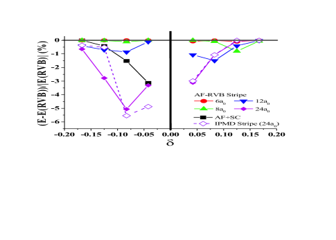
Figure 1: (Color online) The doping dependence of the optimized energy difference in terms of percentage for several trial states denoted in the figure. The reference ground state is the uniform $d$-RVB state. The positive (negative) doping density $\delta$ means the hole-doped (electron-doped) cases. Note that the AF-RVB stripe states with different magnetic periods are indicated. The lattice size $N$ is $24\times 24$. Here $\Lambda=0.25$ and $|t^{\prime}/t|=0.1$.

Figure 1 shows the percentage of energy change with respect to the $d$-RVB state for three other trial wave functions in the extended $t^{\ast}-J$ model with smaller $|t^{\prime}/t|(=0.1)$ for hole- and electron-doped phase diagrams. In the hole-doped case, the half-doped AF-RVB stripe is still observed like our previous studies for $t^{\prime}/t(=-0.2)$ CPCPRB10 . In fact, the half-doped AF-RVB stripe can be always found for all $|t^{\prime}/t|$ we have investigated in the hole-doped region as shown in Fig.3(a) and (b). In other words, the Fermi surface topology seems not to affect the stability of the half-doped stripe obtained in the extended $t^{\ast}-J$ model.

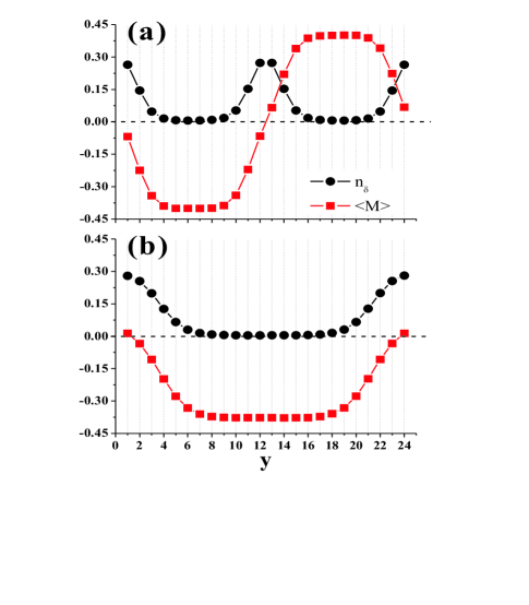
Figure 2: (Color online) The profile of carrier density $n_{\delta}$ and staggered magnetization $\langle M\rangle$ for the optimized states: (a) the AF-RVB stripe and (b) the IPMD stripe with $24a_{0}$ magnetic periodicity at $1/12$ electron-doping in the extended $t^{\ast}-J$ Hamiltonian. The bare parameters $\Lambda=0.25$ and $|t^{\prime}/t|=0.1$. All quantities are calculated in a $24\times 24$ lattice.

In the left panel of Fig.1 we find the IPMD stripe states are stabilized for electron-doping less than $0.1$. For doping greater than $0.1$, the AF-RVB stripe state with the largest magnetic period has the lowest energy ($24a_{0}$ is the largest size we have studied here). The magnetic period does not change with the doping density as the half-doped stripes. We also examine the IPMD stripe states with different periods in addition to $24a_{0}$. The results are not shown here, but the most stable IPMD stripe has the largest magnetic period as lattice size. The difference between the AF-RVB and IPMD stripes for the maximum magnetic period of $24a_{0}$ is actually negligible. Since the IPMD state has much lower energy for doping less than $0.1$, it appears that the $t^{\ast}-J$ Hamiltonian does not prefer to break the system into many $\pi$-phase-shift magnetic domains. In Fig.2(a) and (b) for $1/12$ electron density, the spatial variation of charge density and staggered magnetization along the direction of modulation are shown for the AF-RVB stripe and IPMD stripe, respectively. For both states, there is almost no doped carriers in the region with the strongest staggered magnetization. It is essentially a phase separated state with an electron-rich region and an insulating half-filled AF long-range ordered region. The IPMD stripe state has staggered magnetization $|\langle M\rangle|=0.265$, which is close to the homogeneous AF+SC state ($|\langle M\rangle|=0.269$). This is consistent with the commensurate short-range spin correlations detected by neutron scattering YamadaPRL03 .

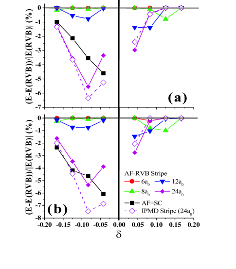
Figure 3: (Color online) The same descriptions are presented in the caption of Fig.1 except for (a) $|t^{\prime}/t|=0.2$ and (b) $|t^{\prime}/t|=0.3$.

For larger $t^{\prime}/t$, we expect robust AF correlations should persist to the higher doping in electron-doped cases. Figure 3 shows this common feature for the uniform AF+SC and the IPMD stripe states. In Fig.3(a), while the homogeneous AF+SC state has much lower energy than the $d$-RVB state, the IPMD stripe state is still the best candidate for electron-doping $\delta<0.1$. It is worth pointing out that for electron-doping $\delta>0.1$ the IPMD stripe state begins to gain energy to compete with the AF-RVB stripe state in the case of $t^{\prime}/t=0.2$. Interestingly, as increasing $t^{\prime}/t(=0.3)$ further, the AF-RVB stripe states entirely disappear in the electron-doped phase diagram possibly due to its $\pi$-phase-shift domains in the spin modulation, as shown in Fig.3(b). Except for the higher electron-doping region ($\delta>0.15$) where the homogeneous AF+SC state still exists, the IPMD stripe state is dominant within the wider doping range ($0<\delta<0.15$). In addition to these stripe states shown in the phase diagram, we have also examined other trial wave functions with different shapes and periods for stripes, such as glassy stripes with randomly-oriented $8\times 8$ magnetic patches, IPMD stripes with other periods, and the diagonal stripe with the largest magnetic period $(12\sqrt{2}a_{0})$. However, none of them can be stabilized for all $t^{\prime}/t$ in electron-doped cases (not shown).

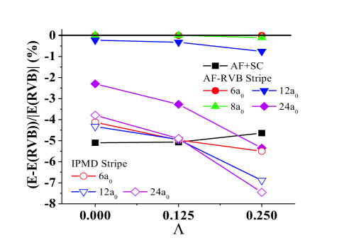
Figure 4: (Color online) $\Lambda$-dependence of the optimized energy difference in terms of percentage for several trial states denoted in the figure at 1/12 doping. Here $N=24\times 24$ and $t^{\prime}/t=0.3$.

To complete the discussion on the VMC results, we study the effect of the electron-phonon coupling strength $\Lambda$ on the phase diagrams. Since the IPMD stripe state has much lower energy near $1/12$ electron-doping, we only show $\Lambda$-dependence of the optimized energy difference for several trial wave functions including IPMD stripes with different magnetic periods at $1/12$ doping in Fig.4. As we expected, the stability of the uniform AF+SC state is almost independent of $\Lambda$ as $\Lambda\lesssim 0.2$. If the electron-phonon coupling strength is smaller $(\Lambda<0.125)$, the AF+SC state would be still a good candidate for the ground state near the underdoped region in the electron-doped side. However, once $\Lambda$ becomes larger, IPMD stripe states begin to be stabilized. Notably, the best one for $\Lambda=0.25$ is either the IPMD stripe state with the largest magnetic period or the phase-separated state. Unlike hole-doped cases, there is no place for AF-RVB stripe states at this doping in electron-doped phase diagrams.

Although the lowest energy solutions of electron-doped systems for the extended $t^{\ast}-J$ Hamiltonian are IPMD stripes and not AF-RVB stripes as the hole-doped systems, the particular patterns of modulation periods of charge density, spin density and pair field for both stripes are derived from the fluctuations of the order parameters used in the mean field theory as shown by using the Gutzwiller approximation. The inhomogeneous states like stripes or phase separation is really due to excitations or fluctuations of order parameters of the ground states of the strongly correlated $t-J$ model. When electron-phonon interaction is introduced to renormalize the mass of carriers, these inhomogeneous solutions then become stable.

In conclusion, following the same approach we have used to study stripes for hole-doped systems CPCPRB08 ; CPCPRB10 , we have further studied the possibilities of having non-uniform ground states for the electron-doped cases using the VMC method. By using the Gutzwiller approximation to examine the fluctuations of order parameters used to obtain the $d$-RVB ground states, we have found that the period of modulation of charge density, staggered moment and pair field are correlated. For hole-doped systems the lowest energy stripes, the AF-RVB stripe states, have the period of staggered moment twice of that of charge and pair field. These stripes with half a carrier per charge domain become the ground states after we include the weak electron-phonon coupling. However, similar approach for electron-doped cases has turned out a different stripe pattern. The lowest energy stripes, the IPMD stripe states, now have the period of staggered moment same as that of charge and pair field. One of the main reasons is that for a large electron doping range the ground state has long-range AF order. The numerical results show that at low doping, the IPMD stripe state with the largest magnetic period same as lattice size is composed of an electron-rich region and an insulating half-filled long-range AF ordered region. We believe that it may indicate a phase separated state in electron-doped compounds. This statement requires the numerical calculation with large lattice size that is left for our future study.

Our result that the electron-doped systems should not have the half-doped stripes observed in hole-doped systems is consistent with the neutron scattering results for cuprates that Yamada plot is only observed for hole-doped cuprates YamadaPRB98 but not for electron-doped ZhaoNatPhys11 . The evidence on magnetic inhomogeneity we have found numerically has been indirectly observed in the electron-doped cuprates $Pr_{2-\delta}Ce_{\delta}CuO_{4}$ and $Pr_{0.88}LaCe_{0.12}CuO_{4-\delta}$ by using $\mu$SR and STS experiments, respectively KlaussJPCM04 ; ZhaoNatPhys11 . The fact that for electron doping we predict possible phase separation which is also a hotly debated issue by experiments on cuprates is quite interesting. We look forward to possible resolution of this issue in the near future.

- (1) J. Tranquada et al., Nature 375, 561 (1995).
- (2) A. Kivelson et al., Rev. Mod. Phys. 75, 1201 (2003).
- (3) K. Yamada, C. H. Lee, K. Kurahashi, J. Wada, S. Wakimoto, S. Ueki, H. Kimura, Y. Endoh, S. Hosoya, G. Shirane, R. J. Birgeneau, M. Greven, M. A. Kastner, and Y. J. Kim, Phys. Rev. B 57, 6165 (1998).
- (4) G. B. Martins, C. Gazza, J. C. Xavier, A. Feiguin, and E. Dagotto, Phys. Rev. Lett. 84, 5844 (2000).
- (5) S. R. White and D. J. Scalapino, Phys. Rev. Lett. 81, 3227 (1998).
- (6) E. Arrigoni, A. P. Harju, W. Hanke, B. Brendel, and S. A. Kivelson, Phys. Rev. B 65, 134503 (2002).
- (7) J. Zaanen and O. Gunnarsson, Phys. Rev. B 40, 7391 (1989).
- (8) V. J. Emery and S. A. Kivelson, Physica C 209, 597 (1993).
- (9) Y. Kohsaka, C. Taylor, K. Fujita, A. Schmidt, C. Lupien, T. Hanaguri, M. Azuma, M. Takano, H. Eisaki, H. Takagi, S. Uchida, and J. C. Davis, Science 315, 1380 (2007).
- (10) C. V. Parker et al., Nature 468, 677 (2010).
- (11) Chung-Pin Chou and Ting-Kuo Lee, Phys. Rev. B 81, 060503(R) (2010).
- (12) N. P. Armitage, P. Fournier, and R. L. Greene, Rev. Mod. Phys. 82, 2421 (2010).
- (13) N. Harima et al., Phys. Rev. B 64, 220507 (2001).
- (14) E. M. Motoyama et al., Phys. Rev. Lett. 96, 137002 (2006).
- (15) K. Yamada et al., Phys. Rev. Lett. 90, 137004 (2003).
- (16) J. Zhao et al., Nat. Phys. 7, 719 (2011).
- (17) J. Sonier et al., Phys. Rev. Lett. 91, 147002 (2003).
- (18) H.-H. Klauss, J. Phys.: Condens. Matter 16, S4457 (2004).
- (19) F. Zamborszky et al., Phys. Rev. Lett. 92, 047003 (2004).
- (20) P. Fournier, et al., Phys. Rev. B 69, 220501(R) (2004).
- (21) X. F. Sun, Y. Kurita, T. Suzuki, S. Komiya, and Y. Ando, Phys. Rev. Lett. 92, 047001 (2004).
- (22) Pengcheng Dai, H. J. Kang, H. A. Mook, M. Matsuura, J. W. Lynn, Y. Kurita, Seiki Komiya, and Yoichi Ando, Phys. Rev. B 71, 100502(R) (2005).
- (23) J. S. Higgins, Y. Dagan, M. C. Barr, B. D. Weaver, and R. L. Greene, Phys. Rev. B 73, 104510 (2006).
- (24) A. Sadori and M. Grilli, Phys. Rev. Lett. 84, 5375 (2000).
- (25) B. Valenzuela, Phys. Rev. B 74, 045112 (2006).
- (26) N. P. Armitage et al., Phys. Rev. Lett. 88, 257001 (2002).
- (27) M. Granath, Phys. Rev. B 69, 214433 (2004).
- (28) Chung-Pin Chou, Noboru Fukushima, and Ting-Kuo Lee, Phys. Rev. B 78, 134530 (2008).
- (29) T. K. Lee, Chang-Ming Ho, and Naoto Nagaosa, Phys. Rev. Lett. 90, 067001 (2003).
- (30) Noboru Fukushima, Phys. Rev. B 78, 115105 (2008).
- (31) Wing-Ho Ko, Cody P. Nave, and Patrick A. Lee, Phys. Rev. B 76, 245113 (2007).
- (32) P. Abbamonte et al., Nat. Phys. 1, 155 (2005).
- (33) H. Yokoyama and H. Shiba, J. Phys. Soc. Jpn. 57, 2482 (1988).
- (34) C.-P. Chou, F. Yang, and T.-K. Lee, arXiv:1110.6399.
- (35) C. T. Shih et al., Chinese J. Phys. 45, 207 (2007).