On maximal globally hyperbolic vacuum space-times

Abstract

We prove existence and uniqueness of maximal global hyperbolic developments of vacuum general relativistic initial data sets with initial data $(g,K)$ in Sobolev spaces $H^{s}\oplus H^{s-1}$, $\mathbb{N}\ni s>n/2+1$.

1 Introduction

One of the many contributions of Yvonne Choquet-Bruhat to the foundations of mathematical general relativity is the proof of the local well-posedness of the initial value problem for the Einstein equations [18], followed by the celebrated Choquet-Bruhat – Geroch theorem [7], which asserts that to every smooth vacuum general relativistic initial data set $(\mycal S,g,K)$ one can associate a unique, up to isometries, smooth solution of the vacuum Einstein equations. Now, there is a gap between the smoothness assumed in this last result and the classical local existence theory [20], where solutions with Sobolev initial data $(\gamma,K)\in H^{s}\oplus H^{s-1}$ are constructed for $s>n/2+1$. The aim of this work is to make a step towards bridging this gap. It is a great pleasure to dedicate the following theorem to Yvonne Choquet-Bruhat for her ninetieth birthday:

Theorem 1.1.

Consider a vacuum Cauchy data set $(\mycal S,\gamma,K)$, where $\mycal S$ is an $n$-dimensional manifold, $\gamma\in H^{s}_{\textrm{\scriptsize loc}}(\mycal S)$ is a Riemannian metric on $\mycal S$, and $K\in H^{s-1}_{\textrm{\scriptsize loc}}(\mycal S)$ is a symmetric two–tensor on $\mycal S$, satisfying the general relativistic vacuum constraint equations, where $\mathbb{N}\ni s>n/2+1$, $n\geq 3$. Then there exists a Lorentzian manifold $({\mycal M},g)$ with a $H^{s}_{{\mathrm{space,loc}}}$-metric, unique up to isometries within the $H^{s}_{{\mathrm{space,loc}}}$ class, inextendible in the class of globally hyperbolic space–times with a $H^{s}_{{\mathrm{space,loc}}}$ vacuum metric and with an embedding $i:\mycal S\rightarrow{\mycal M}$ such that $i^{*}g=\gamma$, and such that $K$ corresponds to the extrinsic curvature tensor of $i(\mycal S)$ in ${\mycal M}$.

We have considered the vacuum Einstein equations for definiteness, similar results can be established for Einstein equations coupled with appropriate matter sources, e.g. for the Einstein-minimally coupled scalar field equations, or the Einstein-Yang-Mills-Higgs equations, or in fact for any quasi-linear systems of wave-equations in space-dimensions $n\geq 1$.

The manifold $({\mycal M},g)$ of the theorem is called the maximal globally hyperbolic vacuum development of $(\mycal S,\gamma,K)$; it is yet another classical result of Yvonne Choquet-Bruhat that $({\mycal M},g)$ is independent of $s$ for $s>n/2+1$.

To avoid ambiguities, global hyperbolicity here is the requirement that every inextendible causal curve meets $i(\mycal S)$ precisely once.

There is little doubt that the condition $\mathbb{N}\ni s>n/2+1$ can be relaxed to $\mathbb{R}\ni s>n/2+1$ using paradifferential techniques, see e.g. [2, 28]. We reduce this question to the problem of verifying conditions H1-A3, p. H1., compare Theorem 3.1 below. It is conceivable that the result generalises to more general classes of initial data for which local existence and uniqueness of solutions holds, such as e.g. those considered in [24, 23, 22, 30, 29, 33, 32], but this remains to be seen.

The proof here is an adaptation of that in [9], using the Planchon-Rodnianski uniqueness argument [30], an extension of the analysis in [4, Appendix A] to Lorentzian manifolds with $H^{s}_{{\mathrm{space,loc}}}$ metrics, and the causality theory for continuous metrics in [13]. In fact, this last work was carried out with the current problem in mind.

It might be useful to comment upon the differentiability thresholds that arise in previous proofs of the theorem. First, all previous proofs use various elements of causality theory which have only been consistently developed using standard approaches for smooth, or $C^{2}$ [11] metrics. So, without further detailed justifications, that part of the proof that appeals to causality theory would require at least $C^{2}$-differentiability of the metric. The original proof in [7] assumes explicitly smoothness at the outset, and invokes existence and uniqueness of geodesics, which fails for metrics which are not $C^{1,1}$. Similarly geodesics are invoked in the proofs given in [19, 31, 8].

This author’s argument in [9] (which proves a more general result concerning orbits of Killing vectors, with the Choquet-Bruhat – Geroch theorem in the smooth category of metrics being a straightforward consequence of Proposition 2.2 there) was presented for smooth metrics because neither the low-differentiability causality theory, nor the Planchon-Rodnianski uniqueness argument [30] were available at the time. As such, the proof in [9] was written using arguments which were expected to generalise to metrics with Sobolev differentiability if the associated causality theory goes through. Inspection of [9] shows that the elements of causality theory needed there arise in the proof of Lemma 2.3 of that reference, and are

1. existence and causality of accumulation curves;

2. the fact that a causal curve which is not null everywhere can be deformed to a timelike curve at end points fixed; and

3. existence of null geodesic generators of $\partial{\mycal D}_{J}$.

It is not obvious, but proved in [13] (see also [16]), that point (1) remains true for continuous metrics, but that point (2) is wrong for continuous metrics; then the usual arguments addressing (3) fail. This part of the argument is replaced by the rather more involved argument starting after the proof of Lemma 3.5, p. 3.5 below.

2 Existence of maximal developments

As a first step in the proof of the Choquet-Bruhat – Geroch theorem, one constructs space-times which are maximal with respect to a set of properties. This begs the question, if and when is such a construction possible. We start by addressing this. Some notation is in order.

Let $W$ denote a set of properties of a manifold, possibly equipped with some supplementary structure such as a metric. Here all manifolds are connected, paracompact, Hausdorff, of at least $C^{1}$-differentiability class. When talking about space-time, the dimension will be denoted by $n+1$. Thus, spacelike hypersurfaces, or their models, will be of dimension $n$. The property $W$ will include differentiability requirements, e.g. $C^{k,\alpha}$, or analyticity, or some Sobolev class, and it might, or might-not, include some further requirements.

A manifold will be said to be Lorentzian if it is equipped with a metric tensor, perhaps defined only almost everywhere, of a differentiability class adapted to $W$. For example, a natural class $W$ could be manifolds with a $C^{k,\alpha}$ atlas, $k\geq 1$, and metrics of $C^{k-1,\alpha}$-differentiability class. It is useful to keep in mind that $W$ can denote a rather complicated structure. For the purpose of the Cauchy problem in general relativity we will be using a $H^{s}_{{\mathrm{space,loc}}}$-structure, defined as follows:

Definition 2.1.

Let $s\in\mathbb{R}$. A Lorentzian manifold $({\mycal M},g)$ will be said to have a metric of $H^{s}_{{\mathrm{space,loc}}}$-differentiability class if every point $p\in{\mycal M}$ has a coordinate neighborhood ${\mycal U}_{p}=I\times{\mycal V}_{p}$, where $I\subset\mathbb{R}$ is the range of a local time coordinate $t\equiv x^{0}$, with the following properties: On every level set $\mycal S_{\tau}\subset{\mycal U}_{p}$ of the coordinate $t$ the metric components $g_{\mu\nu}$ are of $H^{s}$-differentiability class, and their time-derivatives of order $0\leq k\leq\lfloor s\rfloor$ are of $H^{s-k}$-differentiability. Furthermore the functions

$$I\ni t\mapsto\|\partial^{k}_{0}g_{\mu\nu}|_{\mycal S_{t}}\|_{H^{s-k}}\;,\qquad 0\leq k\leq\lfloor s\rfloor\;,$$

are continuous.

Thus, the subscript “space” in $H^{s}_{{\mathrm{space,loc}}}$ denotes the fact that the differentiability of the metric is defined in terms of Sobolev spaces on spacelike hypersurfaces. The subscript “loc”, shorthand for “local”, refers to the fact that the integrals defining the $H^{s}$ norms are finite on conditionally compact sets, but not necessarily so for sets with non-compact closure.

Our results show that the definition is well suited for the problem at hand when $s\in\mathbb{N}$, $s>n/2+1$. It is likely that it will require fine-tuning for other values of $s$.

One expects that the maximal atlas compatible with a $H^{s}_{{\mathrm{space,loc}}}$ structure has transition maps which are of differentiability class $H^{s+1}_{{\mathrm{space,loc}}}$. A version of this, which constitutes one of the elements of the proof of Theorem 1.1, is established in Proposition 3.7 below for $s\in\mathbb{N}$ satisfying $s>n/2+1$.

Since all our manifolds are assumed to be $C^{1}$, maps between them will also be $C^{1}$ in any case, unless explicitly indicated otherwise.

A Lorentzian manifold will be called vacuum if the equations $R_{\mu\nu}=0$ can be defined, perhaps in a distributional sense, and if $R_{\mu\nu}=0$ holds. Note that the Christoffel symbols can be defined for metrics with $g^{\mu\nu}\in L^{\infty}_{\textrm{\scriptsize loc}}$ and which have distributional derivatives in $L^{1}_{\textrm{\scriptsize loc}}$. The equation $R_{\mu\nu}=0$ can be defined in a distributional sense if moreover the distributional derivatives of the metric are in $L^{2}_{\textrm{\scriptsize loc}}$.

The standard theory of PDEs leads to $H^{s}_{{\mathrm{space,loc}}}$-solutions of the Einstein equations with $\mathbb{R}\ni s>n/2+1$, with an atlas in which the coordinate functions are harmonic [20, 30] (compare [12, Section 4.3]).

The work in [24] together with [27, Theorem 7.1] establishes local existence of vacuum metrics in dimension $3+1$ for asymptotically flat initial data on $\mathbb{R}^{3}$ with $\mbox{tr}K=0$ and $(\gamma,K)\in H^{s}_{\textrm{\scriptsize loc}}\times H^{s-1}_{\textrm{\scriptsize loc}}$ with $s>2$; see also [5]. The more recent results of [25] are expected to lower this threshold to $s=2$.

As we will be solving the Cauchy problem, we will need to consider an embedding $i$ of a spacelike hypersurface $\mycal S$ into $({\mycal M},g)$. The embedding should be compatible with the available structures; we will say that $i$ is $W$-compatible when this is the case. For example, for $C^{k,\alpha}$, or smooth, or analytic, manifolds it is natural to consider maps which are also of $C^{k,\alpha}$ class, or smooth, or analytic. So, in this case, a $W$-compatible embedding is required to be $C^{k,\alpha}$, or smooth, etc. For manifolds with $H^{s}_{{\mathrm{space,loc}}}$ metrics it is natural to consider embeddings $i:\mycal S\to{\mycal M}$ such that the pull-backs $(\gamma,K)$ of the metric and of the extrinsic curvature from $i(\mycal S)$ to $\mycal S$ are in $H^{s}_{\textrm{\scriptsize loc}}\otimes H^{s-1}_{\textrm{\scriptsize loc}}$; this is our definition of $W$-compatible embedding for $H^{s}_{{\mathrm{space,loc}}}$ manifolds. The resulting hypersurfaces $i(\mycal S)$ will be called $W$-compatible.

A reader only interested in smooth vacuum space-times can assume that $W$ is the property that $({\mycal M},g)$ is a smooth, Hausdorff, paracompact, connected globally hyperbolic vacuum manifold with a smooth metric. A $W$-compatible embedding $i$ then means that $i$ is smooth and that $i(\mycal S)$ is Cauchy, while a $W$–compatible submanifold means a smooth submanifold. Similarly for $C^{k,\alpha}$ or analytic manifolds.

As such, the next theorem works with any notions of $W$–manifold and $W$–compatible embedding which can be formulated within the framework of set theory as described e.g. in [21, Appendix], under the following proviso: The property $W$ will be said to be chain-inheriting if both the manifold $\,\,\,\,\overline{\!\!\!\!{\mycal M}}$ of (2.2) and the associated embedding $\bar{\imath}$ of $\mycal S$ have the property $W$ whenever all the manifolds $\,\,\,\,\widetilde{\!\!\!\!{\mycal M}}$ in the union there and the embeddings $\tilde{\imath}$ do. An example of chain-inheriting property $W$ is “${\mycal M}$ is a $C^{1}$ manifold with a continuous metric of X-differentiability”, where $X$ stands for $C^{k}$, with $k\in\mathbb{N}\cup\{\infty,\omega\}$, or $C^{k,\alpha}$, or $H^{s}_{{\mathrm{space,loc}}}$, with the corresponding property for the embeddings.

To make things clear, for the purposes of Theorem 1.1 the property $W$ in Theorem 2.2 below is: “$({\mycal M},g)$ is a Hausdorff, paracompact, connected vacuum $C^{1}$ manifold with a Lorentzian metric of $H^{s}_{{\mathrm{space,loc}}}$-differentiability class”. However, we did not formulate the result in this way as Theorem 2.2 has wider applicability, e.g. for the construction of extensions of black-hole exteriors.

We have:

Theorem 2.2.

Let $\mycal S$ be a $n$-dimensional manifold and let $({\mycal M},g,i)$ be a Lorentzian $(n+1)$-dimensional $W$-manifold $({\mycal M},g)$ with a $W$–compatible embedding $i:\mycal S\to{\mycal M}$. Suppose that the property $W$ is chain-inheriting, and that

the only isometry of a $$W ({\mycal M},g)$$-manifold which is the identity

on a $$W$$-compatible hypersurface is the identity map. (2.1)

Then there exists a Lorentzian $W$-manifold $(\,\,\,\,\widetilde{\!\!\!\!{\mycal M}},\tilde{g},\tilde{\imath})$ with a $W$-compatible embedding $\tilde{\imath}:\mycal S\to\,\,\,\,\widetilde{\!\!\!\!{\mycal M}}$ and a $C^{1}$ isometric embedding $\Phi:{\mycal M}\rightarrow\,\,\,\,\widetilde{\!\!\!\!{\mycal M}}$ satisfying $\tilde{\imath}=\Phi\circ i$ such that $\,\,\,\,\widetilde{\!\!\!\!{\mycal M}}$ is inextendible in the class of Lorentzian $W$-manifolds with a $W$-compatible embedding of $\mycal S$.

Remarks 2.3.

1. The $C^{1}$-differentiability threshold for $\mycal S$ and ${\mycal M}$ cannot be weakened in the proof below, since we are using the Whitney embedding theorem to turn the collection of manifolds into a set. The author ignores whether or not the $C^{1}$-differentiability is necessary.

2. One expects the differentiability of $\Phi$ to be determined by that of the metric. For example $\Phi$ will be $C^{k+1,\alpha}$ if the metric is $C^{k,\alpha}$; smooth or analytic if the metric is, etc. This is proved by a bootstrap argument applied to (2.5) below. See [10, Appendix A] for the analytic case.

3. The maximal manifolds $(\,\,\,\,\widetilde{\!\!\!\!{\mycal M}},\tilde{g})$ need not be unique, and may depend upon $W$. A non–trivial example of $W$ dependence, with $W=C^{k,\alpha}$, is given by a class of Robinson–Trautman (RT) space–times studied in [14], which for $k+\alpha\geq 123$ do not admit any non–trivial future extensions, while for $k+\alpha<118$ possess an infinite number of non–isometric vacuum RT extensions.

Proof.

For $\ell\geq n$ let $A_{\ell}$ denote the set of subsets of $\mathbb{R}^{\ell}$ which are $n$–dimensional, paracompact, connected, Hausdorff, $C^{1}$ manifolds, set $A_{\infty}=\cup_{\ell=0}^{\infty}A_{\ell}$. By a famous theorem of Whitney [34] every such manifold can be embedded in $\mathbb{R}^{\ell}$ for some $\ell$, which shows that every manifold has a representative which is an element of $A_{\infty}$. It follows that without loss of generality a manifold can be viewed as an element of $A_{\infty}$, and we shall do so. With this definition the collection of all $C^{1}$ manifolds is $A_{\infty}$, and therefore is a set. It follows from the axioms of set theory that the collection of all $C^{1}$ manifolds which are $W$-manifolds forms a set. Now, a Lorentzian manifold can be identified with a subset of the bundle $T^{0,2}{\mycal M}$ of 2–covariant tensors on ${\mycal M}$. Next, a map $i$ from $\mycal S$ to ${\mycal M}$ can be identified with a subset of the product $\mycal S\times{\mycal M}$. One easily concludes, using the axioms presented in e.g. [21, Appendix], that the collection, say ${\cal M}_{W,\mycal S}$, of Lorentzian $W$-manifolds with a $W$-compatible embedding of $\mycal S$ forms a set.

Let $({\mycal M},g)$ be a Lorentzian $W$-manifold with $W$-compatible embedding $i:\mycal S\to{\mycal M}$. Consider the subset ${\cal M}_{W}(M,g,i)$ of ${\cal M}_{W,\mycal S}$ defined as the set of those Lorentzian manifolds $(\,\,\,\,\widetilde{\!\!\!\!{\mycal M}},\tilde{g},\tilde{\imath})$ with embedding of $\mycal S$ for which there exists an isometric $C^{1}$ embedding $\Phi:{\mycal M}\rightarrow\,\,\,\,\widetilde{\!\!\!\!{\mycal M}}$ with a $W$-compatible embedding $\tilde{\imath}=\Phi\circ i$. On ${\cal M}_{W}(M,g,i)$ we can define a relation $\prec$ as follows: $(\tilde{M},\tilde{g},\tilde{\imath})\prec(\tilde{M}_{1},\tilde{g}_{1},\tilde{\imath}_{1})$ if there exists an isometric $C^{1}$ embedding $\tilde{\Phi}:\,\,\,\,\widetilde{\!\!\!\!{\mycal M}}\rightarrow\,\,\,\,\widetilde{\!\!\!\!{\mycal M}}_{1}$ satisfying $\tilde{\Phi}\circ\tilde{\imath}=\tilde{\imath}_{1}$. We claim that $\prec$ is a partial order. Here the only non-obvious property is antisymmetry, namely if $(\tilde{M},\tilde{g},\tilde{\imath})\prec(\tilde{M}_{1},\tilde{g}_{1},\tilde{\imath}_{1})$ and $(\tilde{M}_{1},\tilde{g}_{1},\tilde{\imath}_{1})\prec(\tilde{M},\tilde{g},\tilde{\imath})$, then $(\tilde{M},\tilde{g},\tilde{\imath})=(\tilde{M}_{1},\tilde{g}_{1},\tilde{\imath}_{1})$. So let $\tilde{\Phi}:\,\,\,\,\widetilde{\!\!\!\!{\mycal M}}\rightarrow\,\,\,\,\widetilde{\!\!\!\!{\mycal M}}_{1}$ and $\tilde{\Phi}_{1}:\,\,\,\,\widetilde{\!\!\!\!{\mycal M}}_{1}\rightarrow\,\,\,\,\widetilde{\!\!\!\!{\mycal M}}$ be the relevant embeddings:

Then $\tilde{\Phi}_{1}\circ\tilde{\Phi}$ is an isometry of $(\,\,\,\,\widetilde{\!\!\!\!{\mycal M}},\tilde{g})$ which is the identity on $\tilde{\imath}(\mycal S)$. By (2.1) the map $\tilde{\Phi}_{1}\circ\tilde{\Phi}$ is the identity on $\,\,\,\,\widetilde{\!\!\!\!{\mycal M}}$, thus $\tilde{\Phi}\circ\tilde{\Phi}_{1}$ is the identity on $\,\,\,\,\widetilde{\!\!\!\!{\mycal M}}_{1}$ as well, proving that $(\tilde{M},\tilde{g},\tilde{\imath})=(\tilde{M}_{1},\tilde{g}_{1},\tilde{\imath}_{1})$ up to isometry, as desired.

If $A\subset{\cal M}_{W}(M,g,i)$ is a chain, define

$$\,\,\,\,\overline{\!\!\!\!{\mycal M}}=\left(\cup_{(\tilde{M},\tilde{g},\tilde{\imath})\in A}\,\,\,\,\widetilde{\!\!\!\!{\mycal M}}\right)/\sim\;,$$ (2.2)

where for $p\in\,\,\,\,\widetilde{\!\!\!\!{\mycal M}}$ and $q\in\,\,\,\,\widetilde{\!\!\!\!{\mycal M}}_{1}$ we set $p\sim q$ iff $q=\Phi(p)$, where $\Phi:\,\,\,\,\widetilde{\!\!\!\!{\mycal M}}\rightarrow\,\,\,\,\widetilde{\!\!\!\!{\mycal M}}_{1}$ is the isometric $C^{1}$ embedding such that $\Phi\circ\tilde{\imath}=\tilde{\imath}_{1}$. It is not too difficult to show that $\,\,\,\,\overline{\!\!\!\!{\mycal M}}$ is a manifold (Hausdorff, paracompact, connected), and a Lorentzian metric $\overline{g}$ can be defined on $\,\,\,\,\overline{\!\!\!\!{\mycal M}}$ in the obvious way. By the chain-inheriting property, $\,\,\,\,\overline{\!\!\!\!{\mycal M}}$ is a $W$-manifold. Since every $\,\,\,\,\widetilde{\!\!\!\!{\mycal M}}$ such that $(\tilde{M},\tilde{g},\tilde{\imath})\in A$ can be embedded in $\,\,\,\,\overline{\!\!\!\!{\mycal M}}$ as

$$\,\,\,\,\widetilde{\!\!\!\!{\mycal M}}\ni p\mapsto[p]_{\sim}\in\,\,\,\,\overline{\!\!\!\!{\mycal M}}\;,$$

it follows that $\,\,\,\,\overline{\!\!\!\!{\mycal M}}$ is an upper bound for $A$. The Kuratowski-Zorn Lemma (cf. e.g. [21]) shows that ${\cal M}_{W}(M,g,i)$ has maximal elements, which had to be established. $\Box$

Before continuing, it appears useful to exhibit classes of space-times in which condition (2.1) is satisfied. The simplest case is that of $C^{k,\alpha}$ manifolds, where $k+\alpha\geq 3$, with $C^{k-1,\alpha}$ metrics, and with $C^{1}$ submanifolds and embeddings:

Proposition 2.4.

Let $({\mycal M},g)$ be a $C^{2,1}$, connected Lorentzian manifold with a $C^{1,1}$ metric, let $\Psi:{\mycal M}\rightarrow{\mycal M}$ be a $C^{1}$ map such that

$$\Psi^{*}g=g\;,\qquad\Psi\big{|}_{S}=\mbox{id}\quad(S\neq\emptyset)\;,$$

where $S$ is either

1. an open set, or

2. $S=\{p\}$ is a point $p\in{\mycal M}$, in which case we further assume that $\Psi^{*}(p)$ is the identity, or

3. a $C^{1}$ submanifold of codimension $1$, in which case we moreover assume that $\Psi$ preserves time-orientation.

Then

$$\Psi=\mbox{id}\;.$$

Remark 2.5.

Note that each of the conditions is necessary, and that in point 1 and 3 neither size nor completeness requirements are imposed on $S$.

Proof.

Suppose first that $S$ is an open set, let $\tilde{S}$ be the largest open set such that $\Psi\big{|}_{\tilde{S}}=\mbox{id}$. Suppose that $\tilde{S}$ is not closed, thus there exists $p\in\partial\tilde{S}$, let ${\mycal O}$ be any neighbourhood of $p$ with a local coordinate system such that $x^{\mu}(p)=0$. Continuous differentiability of $\Psi$ implies, in local coordinates,

$$\Psi^{\mu}(0)=0\;,\quad\frac{\partial\Psi^{\mu}}{\partial x^{\nu}}(0)=\delta^{\mu}_{\nu}\;.$$ (2.3)

From $\Psi^{*}g=g$ one has

$$g_{\alpha\beta}(x)=g_{\mu\nu}\left(\Psi(x)\right)\frac{\partial\Psi^{\mu}}{\partial x^{\alpha}}\frac{\partial\Psi^{\nu}}{\partial x^{\beta}}\;,$$ (2.4)

$$\frac{\partial^{2}\Psi^{\mu}}{\partial x^{\alpha}\partial x^{\beta}}=\Gamma^{\sigma}_{\alpha\beta}(x)\frac{\partial\Psi^{\mu}}{\partial x^{\sigma}}-\Gamma^{\mu}_{\nu\rho}\left(\Psi(x)\right)\frac{\partial\Psi^{\nu}}{\partial x^{\alpha}}\frac{\partial\Psi^{\rho}}{\partial x^{\beta}}\;,$$ (2.5)

where $\Gamma$ denotes the Christoffel symbols of the metric $g$. Indeed, recall that (2.5) is obtained by differentiating (2.4) and algebraic manipulations when $\Psi$ is $C^{2}$.

When $\Psi$ is assumed to be $C^{1}$ only, the same manipulations show that (2.5) holds in a distributional sense. But since the right-hand side is continuous, we conclude that $\Psi$ is $C^{2}$ in any case.

Setting $A^{\alpha}{}_{\beta}\equiv\frac{\partial\Psi^{\alpha}}{\partial x^{\beta}}$, from (2.5) one obtains the following system of ODE’s along rays emanating from the origin:

$$\frac{d\Psi^{\mu}}{dr}=A^{\mu}{}_{\beta}\frac{x^{\beta}}{r}\;,\qquad r=\left(\sum(x^{\alpha})^{2}\right)^{1/2}\;,$$

$$\frac{dA^{\mu}{}_{\beta}}{dr}=\left(\Gamma^{\sigma}_{\alpha\beta}(x)A^{\mu}{}_{\sigma}-\Gamma^{\mu}_{\nu\rho}\left(\Psi(x)\right)A^{\nu}{}_{\alpha}A^{\rho}{}_{\beta}\right)\frac{x^{\alpha}}{r}\;.$$

The initial conditions (2.3) together with uniqueness of solutions of systems of ODE’s imply $\Psi^{\mu}=x^{\mu}$ in ${\mycal O}$, which leads to a contradiction, and shows that $\partial\tilde{S}=\emptyset$, thus $\tilde{S}={\mycal M}$. This proves point 1.

Note that we have also shown that if $\Psi(p)=p$ and $\Psi^{*}(p)=\textrm{id}$, then $\Psi=\textrm{id}$ on a neighborhood ${\mycal O}$ of $p$, hence $\Psi=\textrm{id}$ by point 1, and point 2 is proved as well.

Suppose now that $S$ is a hypersurface, let $p\in S$. Then $\Psi^{*}$ is the identity on $T_{p}S$ and preserves time-orientation. Elementary algebra shows that $\Psi^{*}(p)$ is the identity: Indeed, this is straightforward if $T_{p}S$ is spacelike or timelike. If $S$ is null, let $n,\ell,e_{A}$, $A=2,\ldots,n$, be a basis of $T_{p}{\mycal M}$ such that $n$ and $\ell$ are null, the $e_{A}$’s are ON and orthogonal to $\ell$ and $n$, with $\ell$ and $e_{A}$ tangent to $S$. Then $\Psi^{*}$ is a Lorentz transformation that leaves invariant $\ell$, the $e_{A}$’s, the space spanned by $\ell$ and $n$, and preserves time-orientation, hence is the identity. The result follows now by point 2. $\Box$

Recall thatwave coordinates, often also called harmonic coordinates, are defined by the requirement that $\Box_{g}x^{\mu}=0$, where $\Box_{g}$ denotes the d’Alembert operator of a metric $g$. We have the following “Lipschitz-harmonic” version of Proposition 2.4:

Proposition 2.6.

Let $({\mycal M},g)$ be a globally hyperbolic connected Lorentzian $(n+1)$-dimensional manifold with differentiable spacelike Cauchy surface $\mycal S$. Let $\Psi:{\mycal M}\rightarrow{\mycal M}$ be a time-orientation preserving $C^{1}$ map such that

$$\Psi^{*}g=g\;,\qquad\Psi\big{|}S=\mbox{id}\;.$$

If ${\mycal M}$ can be covered by wave-coordinates patches in which the metric is $C^{0,1}$, then

$$\Psi=\mbox{id}\;.$$

Remark 2.7.

We have chosen the wave-coordinates condition for definitess. The argument applies to any systems of coordinates in which $\Box_{g}x^{\mu}=F^{\mu}(x,g)$ with Lipschitz functions $F^{\mu}$.

Proof.

Equation (2.5), understood distributionally, in coordinates where $g$ is Lipschitz, shows that $\Psi$ is $C^{1,1}$.

Let $p\in\mycal S$, since $\Psi_{*}$ is an isometry and leaves $T_{p}\mycal S$ invariant, it preserves $(T_{p}\mycal S)^{\perp}$. As $\Psi$ preserves time-orientation, $\Psi_{*}$ maps the unit normal to $\mycal S$ to itself. It follows that $\Psi_{*}$ is the identity at $p$. Since $p$ is an arbitrary point on $\mycal S$, we find that $\Psi_{*}$ is the identity on $\mycal S$; in local coordinates, $\partial\Psi^{\mu}/\partial x^{\nu}|S=\delta^{\mu}_{\nu}$.

Let ${\mycal O}$ denote a conditionally compact domain of definition of some wave-coordinates in which the metric is locally Lipschitz, thus

$$0=\Box_{g}x^{\mu}=-g^{\alpha\beta}\Gamma^{\mu}_{\alpha\beta}\;.$$ (2.6)

Let $\mycal S_{{\mycal O};\tau}{}\subset{\mycal O}$ denote the level set within ${\mycal O}$ of a differentiable time function $t$:

$$\mycal S_{{\mycal O};\tau}{}:=\{t=\tau\}\cap{\mycal O}\;.$$

Note that we are not assuming that $t=x^{0}$.

Consider a point $x$ with coordinates $x^{\mu}$ such that $\Psi(x)\in{\mycal O}$. Contracting (2.5) with the inverse metric, and using the wave-coordinates condition, one obtains

$$\Box_{g}\Psi^{\mu}(x) = g^{\alpha\beta}(x)\left(\frac{\partial^{2}\Psi^{\mu}}{\partial x^{\alpha}\partial x^{\beta}}-\Gamma^{\sigma}_{\alpha\beta}(x)\frac{\partial\Psi^{\mu}}{\partial x^{\sigma}}\right)$$ (2.7)

$$= -g^{\alpha\beta}(x)\Gamma^{\mu}_{\nu\rho}\left(\Psi(x)\right)\frac{\partial\Psi^{\nu}}{\partial x^{\alpha}}\frac{\partial\Psi^{\rho}}{\partial x^{\beta}}\;.$$

Setting $\psi^{\mu}:=\Psi^{\mu}-x^{\mu}$, this can be rewritten in the form

$$\Box_{g}\psi^{\mu}(x) = -g^{\alpha\beta}(x)\Gamma^{\mu}_{\nu\rho}\left(x+\psi(x)\right)\left(\frac{\partial\psi^{\nu}}{\partial x^{\alpha}}+\delta^{\nu}_{\alpha}\right)\left(\frac{\partial\psi^{\rho}}{\partial x^{\beta}}+\delta^{\rho}_{\beta}\right)$$ (2.8)

$$= -g^{\alpha\beta}(x)\Gamma^{\mu}_{\nu\rho}\left(x+\psi(x)\right)\frac{\partial\psi^{\nu}}{\partial x^{\alpha}}\left(\frac{\partial\psi^{\rho}}{\partial x^{\beta}}+2\delta^{\rho}_{\beta}\right)$$

$$-\big{(}g^{\alpha\beta}(x)-\underbrace{g^{\alpha\beta}\left(x+\psi(x)\right)\big{)}\Gamma^{\mu}_{\alpha\beta}\left(x+\psi(x)\right)}_{0}\;.$$

Here we have added the last, vanishing term to make it clear that the last line can be estimated, almost everywhere, by a multiple of $|\psi|$ when the metric is Lipschitz.

To continue, we will need:

Lemma 2.8.

If $\psi^{\mu}=0$ on $\mycal S_{{\mycal O};\tau}{}$, then $\psi^{\mu}=0$ on the domain of dependence ${\mycal D}_{J}(\mycal S_{{\mycal O};\tau}{},{\mycal O})$.

Proof.

The argument proceeds via a standard energy inequality, but some care is needed to take into account the low differentiability, and the fact that (2.8) only holds in local coordinates.

Let $\mycal S_{{\mycal O};\tau,n}{}\subset\mycal S_{{\mycal O};\tau}{}$ be an exhaustion of $\mycal S_{{\mycal O};\tau}{}$ by compact submanifolds with smooth boundary. Let $X$ be any differentiable timelike vector field on ${\mycal M}$ and let $T_{\mu\nu}$ be the energy-momentum tensor associated with $\psi$, defined as

$$T_{\mu\nu}:=\sum_{\alpha}\big{(}\partial_{\mu}\psi^{\alpha}\partial_{\nu}\psi^{\alpha}-\frac{1}{2}g^{\sigma\rho}\partial_{\sigma}\psi^{\alpha}\partial_{\rho}\psi^{\alpha}g_{\mu\nu}+\psi^{\alpha}\psi^{\alpha}X_{\mu}X_{\nu}\big{)}\;.$$ (2.9)

Then $T_{\mu\nu}$ is locally Lipschitz.

Consider the domain of dependence ${\mycal D}_{J}(\mycal S_{{\mycal O};\tau,n}{},{\mycal O})$. For smooth metrics, it is well known that this is a set with Lipschitz boundary, which is spacelike or null almost everywhere. The result remains true for continuous metrics, as seen by noting that $\partial{\mycal D}_{J}(\mycal S_{{\mycal O};\tau,n}{},{\mycal O})$ can be written, locally, as an achronal graph. Such graphs are sandwiched between graphs of future- and past light-cones of any of their points, which easily implies the result.

For $t\geq\tau$ define

$$\Omega_{n,t}={\mycal D}^{+}_{J}(\mycal S_{{\mycal O};\tau,n}{},{\mycal O})\cap\{\tau\leq x^{0}\leq t\}\;,$$

$$T_{n}=\sup_{p\in{\mycal D}^{+}_{J}(\mycal S_{{\mycal O};\tau,n}{},{\mycal O})}t(p)\;,$$

$$I_{n}=\{t\in[\tau,T_{n}]:\,\Psi=\textrm{id}\ \mbox{on}\ \Omega_{n,t}\}\;.$$

(Note that $T_{n}<\infty$.) The set $I_{n}$ is not empty, since $\tau\in I_{n}$. Clearly, $I_{n}$ is closed in $[\tau,T_{n}]$. We will show that $I_{n}$ is also open in $[\tau,T_{n}]$, which will prove that

$$\psi=0 {\mycal D}^{+}_{J}(\mycal S_{{\mycal O};\tau,n}{},{\mycal O})$$ on . (2.10)

Let, thus $s\in I_{n}$. Since $\Psi$ is the identity on $\Omega_{n,s}$, there exists $T>s$ such that $\Psi(\Omega_{n,T})\subset{\mycal O}$. Hence (2.8) applies on $\Omega_{n,t}$ for $\tau\leq t\leq T$ and so there exists a constant $C$ such that there we have, almost everywhere,

$$|\nabla_{\mu}T^{\mu}{}_{\nu}| = \bigg{|}\sum_{\alpha}\Box_{g}\psi^{\alpha}\partial_{\nu}\psi^{\alpha}+\nabla_{\mu}(\psi^{\alpha}\psi^{\alpha}X^{\mu}X_{\nu})\bigg{|}$$

$$\leq C(|\psi^{2}|+|\partial\psi|^{2})\;.$$

As already pointed-out, the last term in (2.8) has been estimated by $C|\psi|$ using the fact that the metric is Lipschitz-continuous. The estimation of the remaining terms is straightforward, for example terms of the form $(\partial\psi)^{3}$ in $\nabla_{\mu}T^{\mu}{}_{\nu}$ have been estimated by $C|\partial\psi|^{2}$.

Letting

$$E_{n}(t)=\int_{\mycal S_{{\mycal O};t}{}\cap\,\Omega_{n,T}}T^{\mu}{}_{\nu}X^{\nu}dS_{\nu}\;,$$

and using the Stokes’ theorem for Lipschitz vector fields on Lipschitz domains (see Corollary A.2, Appendix A; compare [15, 26, 17]) one obtains, for some constant $C_{n}$,

$$\forall\ \tau\leq t\leq T\qquad E_{n}(t)\leq C_{n}\int_{\tau}^{t}E_{n}(s)ds\;.$$

Here we have used that $\psi=0$ on $\mycal S_{{\mycal O};\tau}{}$ and, as before, $\partial\psi=0$ on $\mycal S_{{\mycal O};\tau}{}$ as well. Gronwall’s Lemma gives $E_{n}(t)=0$ for $0\leq t\leq T$. This proves that $I_{n}$ is open, and establishes (2.10).

The fact that $\Psi=\textrm{id}$ on ${\mycal D}^{-}_{J}(\mycal S_{{\mycal O};\tau,n}{},{\mycal O})$ is obtained in an identical way.

Since

$$\cup_{n}{\mycal D}_{J}(\mycal S_{{\mycal O};\tau,n}{},{\mycal O})={\mycal D}_{J}(\mycal S_{{\mycal O};\tau}{},{\mycal O})\;,$$

Lemma 2.8 follows. $\Box$

Returning to the proof of Proposition 2.6, let $h$ be any complete Riemannian metric on ${\mycal M}$. Let $p\in\mycal S$, denote by $B_{p}(n)$ the open $h$-distance ball centred at $p$ of radius $n$, and let

$$K_{n}:=\overline{J^{-}(\overline{B_{p}(n)})\cap J^{+}(\overline{B_{p}(n)})}\;.$$

For smooth metrics it is a standard fact that the interior $\mathring{K}_{n}$ of $K_{n}$ is a globally hyperbolic subset of ${\mycal M}$, with Cauchy surface $\mycal S\cap\mathring{K}_{n}$; this can be seen to remain true for continuous metrics using the results in [13]. It also follows from the results in [13] that $\partial K_{n}$ is a Lipschitz topological hypersurface, with $\mathring{K}_{n}$ lying on one side of $\partial K_{n}$. Since $B_{p}(n)\subset\mathring{K}_{n}$ we have

$$\cup_{n}\mathring{K}_{n}={\mycal M}\;.$$

Let $q\in{\mycal M}$, we want to show that $\Psi(q)=q$. There exists $n$ such that $q\in\mathring{K}_{n}$. Compactness shows that $K_{n}$ can be covered by a finite number of conditionally compact wave-coordinates patches ${\mycal U}_{\ell}$, $\ell=1,\ldots,N(n)$, in which the metric is Lipschitz-continuous.

Choose any smooth differentiable structure on ${\mycal M}$ compatible with the $C^{1}$ atlas in which the metric is continuous. By [13] or [16] there exists a smooth Cauchy time function $t$ on ${\mycal M}$ so that $\mycal S=\{t=0\}$. Set

$$J_{n} := \{\tau\in\mathbb{R}:\ \mycal S_{\tau}\cap K_{n}\neq\emptyset\}\;,$$

$$I_{n} := \{\tau\in J_{n}:\ \Psi=\mathrm{id}\ \mbox{ on }\ \mycal S_{\tau}\cap K_{n}\}\;,$$

where $\mycal S_{\tau}$ denotes the $\tau$-level set of $t$. Since causal curves are transverse to the $\mycal S_{\tau}$’s, $J_{n}$ is a closed interval containing the origin; in fact:

$$J_{n}=[\min_{p\in K_{n}}t(p),\max_{p\in K_{n}}t(p)]\;.$$

Now, $I_{n}\neq\emptyset$ as $0\in I_{n}$, and $I_{n}$ is clearly closed in $J_{n}$. We wish to show that $I_{n}=J_{n}$, hence $\Psi$ is the identity on $K_{n}$. For this, it remains to show that $I_{n}$ is open.

Let then $t\in I_{n}$, and consider those ${\mycal U}_{\ell}$’s that intersect $\mycal S_{t}$, renumbering we can assume that this happens for $\ell=1,\ldots,N$ for some $N=N(t)$. Then $\Psi$ is the identity on $\mycal S_{{\mycal U}_{\ell};t}{}$ for all $\ell=1,\ldots,N$ so that, by Lemma 2.8, the map $\Psi$ is the identity on

$$\cup_{\ell=1}^{N}{\mycal D}_{J}(\mycal S_{{\mycal U}_{\ell};t}{},{\mycal U}_{\ell})\;.$$

We claim that for $t^{\prime}$ close enough to $t$ we have

$$\mycal S_{t^{\prime}}\cap K_{n}\subset\cup_{\ell=1}^{N}{\mycal D}_{J}(\mycal S_{{\mycal U}_{\ell};t}{},{\mycal U}_{\ell})\;.$$ (2.11)

Indeed, suppose that this is not the case, then there exists a sequence $t_{i}\to t$ and points $q_{i}\in\mycal S_{t_{i}}\cap K_{n}$ such that $q_{i}$ does not belong to the set appearing at the right-hand side of the inclusion (2.11). By compactness, passing to a subsequence if necessary, $q_{i}$ converges to $q\in\mycal S_{t}\cap K_{n}$. Then $q\in\mycal S_{{\mycal U}_{\ell};t}{}$ for some $\ell$. But ${\mycal D}_{J}(\mycal S_{{\mycal U}_{\ell};t}{},{\mycal U}_{\ell})$ forms a neighborhood of $\mycal S_{{\mycal U}_{\ell};t}{}$, and so $q_{i}\in{\mycal D}_{J}(\mycal S_{{\mycal U}_{\ell};t}{},{\mycal U}_{\ell})$ for all $i$ large enough, which gives a contradiction.

So (2.11) holds for all $t^{\prime}$ close enough to $t$, which establishes openness of $I_{n}$, and finishes the proof of Proposition 2.6. $\Box$

One can use [20, Theorem III] to cover a manifold with a $H^{s}_{{\mathrm{space,loc}}}$ metric, $s>n/2+1$, by wave-map coordinate patches. However, when transformed to wave-coordinates, the metric will be of $H^{s-1}_{{\mathrm{space,loc}}}$-differentiability class only in general. The requirement of existence of the embedding $H^{s-1}\subset C^{0,1}$ leads to the threshold $s>n/2+2$ for the applicability of Proposition 2.6 for general $H^{s}_{{\mathrm{space,loc}}}$ metrics.

On the other hand, solutions of the vacuum Einstein equations can be constructed directly by patching-together domains of definition of wave-coordinates [29, 30], and then Proposition 2.6 applies without loss of differentiability for the metric when $s>n/2+1$.

3 Global uniqueness

3.1 An abstract theorem

In the context of $H^{s}_{{\mathrm{space,loc}}}$-Lorentzian manifolds, a hypersurface $S$ will be said to be compatible if $S$ is a coordinate-level set of a coordinate system in which the metric is of $H^{s+1}_{{\mathrm{space,loc}}}$-differentiability class.

We will prove a somewhat more general version of Theorem 1.1, where the differentiability index $s\in\mathbb{R}$ is only assumed to satisfy $s>n/2$, as needed to ensure continuity of the metric, provided that the following conditions hold:

1. The harmonically-reduced vacuum Einstein equations with initial data in $H^{s}_{\textrm{\scriptsize loc}}(S)\times H^{s-1}_{\textrm{\scriptsize loc}}(S)$, $S\subset\{t=0\}\subset\mathbb{R}^{n+1}$ have local solutions.

2. Two solutions $g_{1}$ and $g_{2}$ in $H^{s}_{{\mathrm{space,loc}}}$ globally coordinatized by harmonic coordinates with the same data on $S\subset\{t=0\}\subset\mathbb{R}^{n+1}$ coincide on ${\mycal D}_{J,g_{1}}(S)\cap{\mycal D}_{J,g_{2}}(S)$.

3. A time-orientation-preserving $C^{1}$ isometry of $({\mycal M},g)$, with $g\in H^{s}_{{\mathrm{space,loc}}}$, which is the identity on the initial data hypersurface is the identity everywhere.

4. Let $\Phi$ be a $C^{1}$ isometry of two Lorentzian manifolds with $H^{s}_{{\mathrm{space,loc}}}$ metrics. Then $\Phi$ is of $H^{s+1}_{{\mathrm{space,loc}}}$-differentiability class.

5. For any compatible spacelike acausal hypersurface $S$ and for any initial data $(\psi,\chi)\in H^{s+1}_{\textrm{\scriptsize loc}}(S)\times H^{s}_{\textrm{\scriptsize loc}}(S)$ the Cauchy problem

   $$\Box_{g}f=0\;,\qquad f|_{S}=\psi\;,\quad\partial f|_{S}=\chi\;,$$

   has a unique solution of $H^{s+1}_{{\mathrm{space,loc}}}$-differentiability class in the $J$-domain of dependence of $S$.

6. If $\Psi$ is of $H^{s+1}_{{\mathrm{space,loc}}}$-differentiability class and $g$ is in $H^{s}_{{\mathrm{space,loc}}}$, then $\Psi^{*}g$ is in $H^{s}_{{\mathrm{space,loc}}}$.

We note that H1-H2 and A2-A3 are needed for local existence and uniqueness of solutions near the initial data hypersurface. Hypothesis A0  is used in the proof of existence of maximal developments. The hypothesis A1 is used to extend isometries in the proof of uniqueness of maximal globally hyperbolic developments.

We claim that:

Theorem 3.1.

Under the remaining hypotheses of Theorem 1.1, suppose instead that $\mathbb{R}\ni s>n/2$. If moreover the hypotheses H1, H2, and A0-A3 hold, then the conclusions of Theorem 1.1 hold.

The key to the proof is the following proposition:

Proposition 3.2.

Let $s>n/2$, let $({\mycal M}_{a},g_{a})$, $a=1,2$, be vacuum globally hyperbolic $H^{s}_{{\mathrm{space,loc}}}$ space-times with $C^{1}$ Cauchy surfaces $\mycal S_{a}$ and with $H^{s}_{{\mathrm{space,loc}}}\times H^{s-1}_{{\mathrm{space,loc}}}$ initial data, and suppose that (${\mycal M}_{2},g_{2}$) is maximal. Let ${\mycal O}\subset{\mycal M}_{1}$ be a globally hyperbolic neighborhood of $\mycal S_{1}$, with Cauchy surface $\mycal S_{1}$, and suppose there exists an injective time-orientation preserving isometry $\Psi_{{\mycal O}}:{\mycal O}\rightarrow{\mycal M}_{2}$, such that $\Psi_{{\mycal O}}(\mycal S_{1})$ is acausal. If the hypotheses H2 and A1-A3  hold, then there exists an injective isometry

$$\Psi:{\mycal M}_{1}\rightarrow{\mycal M}_{2},$$ (3.1)

such that $\Psi|_{{\mycal O}}=\Psi_{{\mycal O}}$.

Before passing to the proof of Proposition 3.2, let us note that Theorem 3.1 is a corollary thereof:

Proof of Theorem 3.1: The existence of some vacuum globally hyperbolic development, and uniqueness-up-to-isometry in a globally hyperbolic neighborhood of $i(\mycal S)$, are standard consequences of hypotheses H1, H2, A2 and A3. The existence of maximal vacuum globally hyperbolic developments follows from hypothesis A0  and Theorem 2.2.

It should be clear from Proposition 3.2 that two maximal vacuum globally hyperbolic developments are isometrically diffeomorphic: Indeed, let $({\mycal M}_{a},g_{a},i_{a})$, $a=1,2$, be two such developments, with $\mycal S_{a}=i_{a}(\mycal S)$. Let ${\mycal O}_{a}\subset{\mycal M}_{a}$ be isometric globally hyperbolic neighborhoods of $i(\mycal S_{a})$, with injective time-orientation preserving isometries $\Psi_{{\mycal O}_{1}}:{\mycal O}_{1}\to{\mycal O}_{2}$, $\Psi_{{\mycal O}_{2}}:{\mycal O}_{2}\to{\mycal O}_{1}$, the existence of which has just been pointed out. Proposition 3.2 provides injective isometries

$$\Psi_{1}:{\mycal M}_{1}\rightarrow{\mycal M}_{2}\;,\quad\Psi_{2}:{\mycal M}_{2}\rightarrow{\mycal M}_{1}\;.$$ (3.2)

The construction so far gives, in fact, $\Psi_{a}|_{{\mycal O}_{a}}=\Psi_{{\mycal O}_{a}}$, $\Psi_{1}\circ i_{1}=i_{2}$, and $\Psi_{2}\circ i_{2}=i_{1}$. This implies that $\Psi_{2}\circ\Psi_{1}$ is the identity on $\mycal S_{1}$, and thus $\Psi_{1}$ and $\Psi_{2}$ are inverse to each other by hypothesis A0. $\Box$

To complete the proof of Theorem 3.1 it remains to establish Proposition 3.2:

Proof of Proposition 3.2: The condition that $s>n/2$ guarantees that the metric is continuous, and so the causality theory of [13] with continuous metrics applies.

Consider the collection ${{\cal X}}$ of all pairs $({{\mycal U}},\Psi_{{\mycal U}})$, where ${{\mycal U}}\subset{\mycal M}_{1}$ is a neighborhood of $\mycal S_{1}$ such that $\mycal S_{1}$ is a Cauchy surface for $({{\mycal U}},g_{1}|_{{{\mycal U}}})$, and where $\Psi_{{{\mycal U}}}:{{\mycal U}}\rightarrow{\mycal M}_{2}$ is an isometric diffeomorphism between ${{\mycal U}}$ and $\Psi_{{{\mycal U}}}({{\mycal U}})\subset{\mycal M}_{2}$ satisfying

$$\Psi_{{{\mycal U}}}|_{{\mycal O}}=\Psi_{{\mycal O}}\;.$$ (3.3)

The collection ${\cal{X}}$ can be partially ordered by inclusion: $({{\mycal U}},\Psi_{{{\mycal U}}})\leq({\cal{V}},\Psi_{{\cal{V}}})$ if ${{\mycal U}}\subset{\cal{V}}$ and if $\Psi_{{\cal{V}}}|_{{{\mycal U}}}=\Psi_{{{\mycal U}}}$. Let $({{\mycal U}}_{\alpha},\Psi_{\alpha})_{\alpha\in\Omega}$ be a chain in ${\cal{X}}$, set ${\cal{W}}=\cup_{\alpha\in\Omega}{{\mycal U}}_{\alpha}$, define $\Psi_{{\cal{W}}}:{\cal{W}}\rightarrow{\mycal M}_{2}$ by $\Psi_{{\cal{W}}}|_{{{\mycal U}}_{\alpha}}=\Psi_{\alpha}$; clearly (${\cal{W}},\Psi_{{\cal{W}}}$) is a majorant for $({{\mycal U}}_{\alpha},\Psi_{\alpha})_{\alpha\in\Omega}$. As in the proof of Theorem 2.2, using the set-theory axioms from [21, Appendix] it can be seen that ${{\cal X}}$ forms a set, we can thus apply the Kuratowski-Zorn Lemma [21] to infer that there exist maximal elements in ${{\cal X}}$.

Let then $({\,\,\,\,\widetilde{\!\!\!\!{\mycal M}}},\Psi)$ be any maximal element, by definition (${\,\,\,\,\widetilde{\!\!\!\!{\mycal M}}},g_{1}|_{{\,\,\,\,\widetilde{\!\!\!\!{\mycal M}}}}$) is thus globally hyperbolic with Cauchy surface $\mycal S_{1}$, and $\Psi$ is a one-to-one isometry from ${\,\,\,\,\widetilde{\!\!\!\!{\mycal M}}}$ into ${\mycal M}_{2}$ such that

$$\Psi|_{{\mycal O}}=\Psi_{{\mycal O}}\;.$$ (3.4)

We conclude that without loss of generality we can assume that $({\mycal O},\Psi_{{\mycal O}})$ is maximal. We then have:

Lemma 3.3.

Under the hypotheses of Proposition 3.2, suppose that $({\mycal O},\Psi_{{\mycal O}})$ is maximal. Then the topological space

$${\mycal M}^{\prime}=({\mycal M}_{1}\sqcup{\mycal M}_{2})/\Psi_{{\mycal O}}$$

is Hausdorff, hence a manifold.

Remark 3.4.

Recall that $\sqcup$ denotes the disjoint union, while $({\mycal M}_{1}\sqcup{\mycal M}_{2})/\Psi$ is the quotient space $({\mycal M}_{1}\sqcup{\mycal M}_{2})/\sim,$ where $p_{1}\in{\mycal M}_{1}$ is equivalent to $p_{2}\in{\mycal M}_{2}$ if $p_{2}=\Psi(p_{1})$, with the quotient topology.

Proof.

Let $p^{\prime},q^{\prime}\in{\mycal M}^{\prime}$ be such that there exist no open neighborhoods separating $p^{\prime}$ and $q^{\prime}$; clearly this is possible only if, interchanging $p$ with $q$ if necessary, we have $p^{\prime}=[p]$, with $p\in\partial{\mycal O}$ and $q^{\prime}=[q]$, with $q\in\partial\Psi_{{\mycal O}}({{\mycal O}})$. Such points $p$, $p^{\prime}$, $q$ and $q^{\prime}$ will be called “non-Hausdorff”.

Let ${\cal H}$ denote the set of non-Hausdorff points $p$ in ${\mycal M}_{1}$, thus $p^{\prime}=i_{{\mycal M}_{1}}(p)\equiv[p]$ is non-Hausdorff in ${\mycal M}^{\prime}$, where $i_{{\mycal M}_{1}}$ denotes the embedding of ${\mycal M}_{1}$ into ${\mycal M}^{\prime}$. By elementary topology ${\cal H}$ is closed (as its complement is open), and we have just seen that ${\cal H}\subset\partial{\mycal O}$.

Suppose that ${\cal H}\not=\emptyset$, changing time orientation if necessary we may assume that ${\cal H}\cap I^{+}(\mycal S_{1})\neq\emptyset$. Let $\hat{p}\in{\cal H}\cap I^{+}(\mycal S_{1})$. We wish to show that there necessarily exists $p\in{\cal H}$ such that

$${J}^{-}(p)\cap{\cal H}\cap I^{+}(\mycal S_{1})=\{p\}.$$ (3.5)

If (3.5) holds with $p=\hat{p}$ we are done, otherwise consider the (non-empty) set ${\cal{Y}}$ of future directed causal paths $\Gamma:[0,1]\rightarrow I^{+}(\mycal S)$ such that $\Gamma(0)\in{\cal H},\Gamma(1)=\hat{p}$. ${\cal{Y}}$ is directed by inclusion: $\Gamma_{1}<\Gamma_{2}$ if $\Gamma_{1}([0,1])\subset\Gamma_{2}([0,1])$. Let $\{\Gamma_{\alpha}\}_{\alpha\in\Omega}$ be a chain in ${\cal Y}$, we let $\Gamma$ be the causal curve the image of which is the union of the images of all the $\Gamma_{\alpha}([0,1])$’s. Clearly $\Gamma\subset J^{+}(\mycal S_{1})=I^{+}(\mycal S_{1})\cup\mycal S_{1}$, and global hyperbolicity implies that $\Gamma$ must be extendible, thus $\{\Gamma_{\alpha}(0)\}$ accumulates at some $p_{*}\in I^{+}(\mycal S_{1})\cup\mycal S_{1}$. As ${\mycal O}$ is an open neighborhood of $\mycal S_{1}$ the case $p_{*}\in\mycal S_{1}$ is not possible, hence $p_{*}\in I^{+}(\mycal S_{1})$ and consequently $\Gamma\in{\cal{Y}}$. It follows that every chain in ${\cal Y}$ has a majorant, and by Zorn’s Lemma ${\cal Y}$ has maximal elements. Let then $\Gamma$ be any maximal element of ${\cal Y}$, setting $p=\Gamma(0)$ the equality (3.5) must hold.

We now claim that (3.5) also implies that there exists an open neighborhood $\widehat{{\cal V}}$ of $p$ such that

$${J}^{-}(p)\cap\partial{\mycal O}\cap I^{+}(\mycal S_{1})\cap\widehat{{\cal V}}=\{p\}.$$ (3.6)

In order to establish (3.6), we start with the following lemma (recall that our notation and terminology follow [13]):

Lemma 3.5.

Let $p\in\partial{\mycal O}\cap J^{+}(\mycal S_{1})$, then ${\check{I}{}}^{-}(p)\cap J^{+}(\mycal S_{1})\subset{\mycal O}$.

Remark 3.6.

For $C^{0,1}$ metrics one has $I^{-}(p)={\check{I}{}}^{-}(p)$ [13], and then the result is standard. We do not know whether the inclusion $I^{-}(p)\cap J^{+}(\mycal S_{1})\subset{\mycal O}$ holds for metrics which are merely continuous.

Proof.

Let $q\in{\check{I}{}}^{-}(p)\cap J^{+}(\mycal S_{1})$, then $p\in{\check{I}{}}^{+}(q)$, and so ${\check{I}{}}^{+}(q)$ forms an open neighborhood of $p$. Let $p_{i}\in{\mycal O}$ be a sequence converging to $p$, then $p_{i}\in{\check{I}{}}^{+}(q)$ for $i$ large enough. Let $\gamma_{i}$ be a timelike curve from $p_{i}$ to $q$, note that $\gamma_{i}$ does not meet $\mycal S_{1}$ since $q\in I^{+}(\mycal S_{1})$ and $\mycal S_{1}$ is achronal. Let $\hat{\gamma}_{i}$ be any past inextendible causal extension of $\gamma_{i}$. Global hyperbolicity implies that $\hat{\gamma}_{i}$ is included in ${\mycal O}$ at least until it meets $\mycal S_{1}$ when followed to the past from $p_{i}$, hence $q\in{\mycal O}$. $\Box$

Returning to the proof of (3.6), let $\gamma_{p}$ be a past-inextendible locally uniformly timelike curve with $p=\gamma_{p}(0)$; by global hyperbolicity and Lemma 3.5 the curve $\gamma_{p}$ meets $\mycal S_{1}$ at, say, $\gamma_{p}(1)$. Thus $p\in{\check{I}{}}^{+}(\gamma_{p}(1))$; since the last set is open, there exists an open neighborhood $\widehat{{\cal V}}$ of $p$ contained in ${\check{I}{}}^{+}(\gamma_{p}(1))$.

Suppose that (3.6) is wrong, then there exists a point

$$q\in{J}^{-}(p)\cap\partial{\mycal O}\cap I^{+}(\mycal S_{1})\cap\widehat{{\cal V}}\subset{J}^{-}(p)\cap\partial{\mycal O}\cap{\check{I}{}}^{+}(\gamma_{p}(1))$$

which is distinct from $p$.

Let $\gamma_{q}$ be a past inextendible $g$-causal curve starting at $q$. By Lemma 3.5 points on $\gamma_{p}$ distinct from $p$, and on $\gamma_{q}$ distinct from $q$, and lying to the future of $\mycal S_{1}$ are in ${\mycal O}$.

Let $q_{i}\neq q$ be any sequence of points on $\gamma_{q}$ converging to $q$ such that $q_{i+1}\ni{\check{I}{}}^{+}_{g_{1}}(q_{i})$. In particular $q_{i}\in{\mycal O}$. The aim of the argument is to show that $\Psi_{\mycal O}(q_{i})$ has a limit in ${\mycal M}_{2}$, which will imply that $q\in\cal H$, a contradiction with (3.5). The standard proof [11, 13] of existence of the limit of the sequence $\Psi_{\mycal O}(q_{i})$ for $C^{0,1}$ metrics uses Lemma 3.5 together with the fact that a causal curve which is not everywhere null can be deformed, with end points fixed, to a timelike one. However, there exist continuous Lorentzian metrics and causal curves for which no such deformations exist [13], and a different line of thought is needed.

By [16] there exists a smooth metric ${\hat{g}}_{1}\succ g_{1}$ on ${\mycal M}_{1}$ so that ${\mycal M}_{1}$ is globally hyperbolic with Cauchy surface $\mycal S_{1}$. For $i\geq 2$ let ${\hat{g}}_{i}$ be any sequence of smooth metrics converging locally uniformly to $g_{1}$ such that

$${\hat{g}}_{1}\succ{\hat{g}}_{i}\succ{\hat{g}}_{i+1}\succ g_{1}\;.$$

Then all the spacetimes $({\mycal M}_{1},{\hat{g}}_{i})$ are globally hyperbolic with Cauchy surface $\mycal S_{1}$.

For any $i\geq 2$ and $j\in\mathbb{N}$, the closed null Lipschitz hypersurfaces $\partial J^{+}_{{\hat{g}}_{i}}(q_{j})$ separate ${\mycal M}_{1}$, with $\mycal S_{1}$ lying to their past. Moreover, $p$ cannot lie to the ${\hat{g}}_{i}$-causal past of $\partial J^{+}_{{\hat{g}}_{i}}(q_{j})$: Otherwise, there would be a ${\hat{g}}_{i}$-timelike curve from $\partial J^{+}_{{\hat{g}}_{i}}(q_{j})$ to $p$, which could be concatenated with the $g$-causal curve from $p$ to $q$ (which is ${\hat{g}}_{i}$-timelike), and then deformed to a ${\hat{g}}_{i}$-timelike curve from $\partial J^{+}_{{\hat{g}}_{i}}(q_{j})$ to $p$. Hence either $p\in\partial J^{+}_{{\hat{g}}_{i}}(q_{j})$, or $p$ lies to the timelike future of $\partial J^{+}_{{\hat{g}}_{i}}(q_{j})$. The former case cannot occur, since for the smooth globally hyperbolic metrics satisfying ${\hat{g}}_{i}\succ{\hat{g}}_{i+1}$ one has

$$\partial J^{+}_{{\hat{g}}_{i+1}}(q_{j})\setminus\{q_{j}\}\subset I^{+}_{{\hat{g}}_{i}}\big{(}\partial J^{+}_{{\hat{g}}_{i}}(q_{j})\big{)}\;.$$

The curve $\gamma_{p}$ intersects each of the $\partial J^{+}_{{\hat{g}}_{i}}(q_{j})$’s: indeed, $\gamma_{p}$ has to exit the compact set $J^{-}_{{\hat{g}}_{i}}(p)\cap J^{+}_{{\hat{g}}_{i}}(q_{j})$; since $\partial J^{-}_{{\hat{g}}_{i}}(p)$ is achronal, it can only do so through $\partial J^{+}_{{\hat{g}}_{i}}(q_{j})$. One can then construct a ${\hat{g}}_{i}$-causal curve $\gamma_{j,i}$ from $p$ to $q_{j}$ by following $\gamma_{p}$ from $p$ to its intersection point with $\partial J^{+}_{{\hat{g}}_{i}}(q_{j})$, and then following a generator of $\partial J^{+}_{{\hat{g}}_{i}}(q_{j})$ until $q_{j}$ is reached. For each $j$ the curves $\gamma_{j,i}$ are ${\hat{g}}_{1}$-causal, and $({\mycal M}_{1},{\hat{g}}_{1})$ is globally hyperbolic, therefore there exists a ${\hat{g}}_{1}$-causal curve $\gamma_{j}$ from $q_{j}$ to $p$ which is an accumulation curve of the $\gamma_{j,i}$’s. The curve $\gamma_{j}$ is $g_{1}$-causal by [Theorem 1.6][13].

By Lemma 3.5 the curves $\gamma_{j}$ are included in ${\mycal O}$ except for their end-point $p$. It is convenient to parameterize the $\gamma_{j}$’s by distance from $q_{j}$ with respect to an auxiliary complete Riemannian metric on ${\mycal M}_{2}$. Let $s_{i}$ be defined as $p=\gamma_{i}(s_{i})$.

Denote by $q\in{\mycal M}_{2}$ the non-Hausdorff partner of $p$. Then the curve in ${\mycal M}_{2}$ defined as

$$\hat{\gamma}_{i}:=\Psi_{\mycal O}\circ\gamma_{i}|_{[0,s_{i})}$$

is a $g_{2}$-causal curve lying in the compact set (see [Theorem 2.9.9][11])

$$J^{-}_{g_{2}}(q)\cap J^{+}_{g_{2}}\big{(}\Psi_{\mycal O}(q_{1})\big{)}\subset{\mycal M}_{2}\;.$$

Hence $\hat{\gamma}_{i}$ has an accumulation point, say $\hat{r}_{i}$, lying on the boundary of $\Psi_{\mycal O}({\mycal O})$. The points $r_{i}$ and $\hat{r}_{i}$ form a non-Hausdorff pair, which is only compatible with (3.5) if $\hat{r}_{i}=q$. So, in fact, $\hat{\gamma}_{i}$ can be extended to a causal curve from $\Psi_{\mycal O}(q_{i})$ to $q$ by adding the end point. We will denote by the same symbol that extension.

By global hyperbolicity of ${\mycal M}_{2}$, passing to a subsequence if necessary, the sequence $\hat{\gamma}_{i}$ accumulates at a $g_{2}$-causal curve $\hat{\gamma}$. This shows that the sequence

$$\Psi_{\mycal O}(q_{i})=\hat{\gamma}_{i}(0)$$

has a limit point in ${\mycal M}_{2}$. Hence $q\in\cal H$, which contradicts (3.5). We conclude that (3.6) must hold.

To continue, let $p_{1}\in{\mycal M}_{1}$, $p_{2}\in{\mycal M}_{2}$, be any non-Hausdorff pair in ${\mycal M}^{\prime}$ such that (3.5) holds with $p=p_{1}$. We wish to show that the isometry $\Psi_{\mycal O}$ can be extended near $p_{1}$, which will lead to a contradiction. For this, around $p_{2}$ we can construct harmonic coordinates $y^{\mu}$ as follows: Let $z^{\mu}$ be local coordinates defined in some neighborhood ${\mycal O}_{2}$ of $p_{2}$, such that the metric coefficients are of $H^{s}_{{\mathrm{space,loc}}}$-differentiability class; such coordinates will be said to be $H^{s}_{{\mathrm{space,loc}}}$-compatible. We can, and will, further assume that $z^{0}(p_{2})=0$, and that the level sets of $z^{0}$ are spacelike and acausal near $p_{2}$. Set

$${\cal{I}}_{\tau}=\{q\in{\mycal O}_{2}:z^{0}(q)=\tau\}\;.$$

Passing to a subset of ${\mycal O}_{2}$ if necessary we may assume that ${\mycal O}_{2}$ is globally hyperbolic with Cauchy surface ${\cal{I}}_{0}$. By hypothesis A2  there exist functions $y^{\mu}\in H^{s+1}_{{\mathrm{space,loc}}}$, (unique) solutions of the problem

$$\Box_{g_{2}}y^{\mu}=0,$$

$$y^{0}\big{|}_{{\cal{I}}_{0}}=0,\quad{\partial y^{0}\over\partial z^{0}}\bigg{|}_{{\cal{I}}_{0}}=1,\quad y^{i}\big{|}_{{\cal{I}}_{0}}=z^{i},\quad{\partial y^{i}\over\partial z^{0}}\bigg{|}_{{\cal{I}}_{0}}=0\;.$$ (3.7)

Passing once more to a globally hyperbolic subset of ${\mycal O}_{2}$ if necessary, the functions $y^{\mu}$ form a coordinate system on ${\mycal O}_{2}$.

Let $w^{\mu}$ be any $H^{s}_{{\mathrm{space,loc}}}$-compatible coordinates near $p_{1}$ with domain of definition ${\cal V}\subset\widehat{{\cal V}}$, with $\widehat{{\cal V}}$ as in (3.6). We can choose $\epsilon>0$ such that (see Figure 3.1)

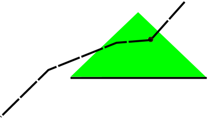
Figure 3.1: Extending the isometry $\Psi_{\mycal O}$ near a spacelike point of $\partial{\mycal O}$. The point $p_{1}$ is located at the dot, the dashed line is $\partial{\mycal O}$, the set ${\mycal O}$ lies under that line; the light cones have $45^{\circ}$ slopes. The shaded region (green in a version with colours) is the future domain of dependence of $\hat{\cal{I}}$.

1. ${\mycal D}^{+}_{J}({\cal{I}}_{-\epsilon})\subset{\mycal O}_{2}$,

2. $p_{2}\in\mbox{int}{\mycal D}^{+}_{J}({\cal{I}}_{-\epsilon})$,

3. $\overline{{\cal{I}}_{-\epsilon}}\subset\Psi_{\mycal O}({\mycal O})$.

Choose any smooth spacelike acausal hypersurface ${\hat{\cal{I}}}$ included in ${\cal V}$ such that

$$\overline{\hat{\cal{I}}}\subset{\mycal D}^{+}_{J}(\Psi^{-1}_{\mycal O}({\cal{I}}_{-\epsilon}))\ \mbox{ and }\ p_{1}\in{\mycal D}^{+}_{J}(\hat{\cal{I}})\;.$$

Now, $\Psi^{-1}_{\mycal O}$ is of $H^{s+1}_{{\mathrm{space,loc}}}$-differentiability class by hypothesis A1. We can thus invoke hypothesis A2 to define on ${\mycal D}_{J}({\hat{\cal{I}}})$ the functions $x^{\mu}\in H^{s+1}_{{\mathrm{space,loc}}}({\mycal D}_{J}(\hat{\cal{I}}))$ as the unique solutions of the problem

$$\Box_{g_{1}}x^{\mu}=0,$$

$$x^{\mu}\big{|}_{\hat{\cal{I}}}=y^{\mu}\circ\Psi_{\mycal O}\big{|}_{{\hat{\cal{I}}}},\quad{\partial x^{\mu}\over\partial{\hat{n}}}\Big{|}_{\hat{\cal{I}}}={\partial\left(y^{\mu}\circ\Psi_{\mycal O}\right)\over\partial\hat{n}}\Big{|}_{\hat{\cal{I}}}\;,$$

where ${\partial\over\partial{\hat{n}}}$ is the derivative in the direction normal to ${\hat{\cal{I}}}$.

By isometry-invariance and by the uniqueness part of hypothesis A2 we have

$$x^{\mu}|_{{\mycal D}_{J}({\hat{\cal{I}}})\cap{\mycal O}}=y^{\mu}\circ\Psi_{\mycal O}|_{{\mycal D}_{J}({\hat{\cal{I}}})\cap{\mycal O}}\;.$$ (3.8)

Equivalently, when expressed in terms of local coordinates $x^{\mu}$ near $p_{1}$ and $y^{\mu}$ near $p_{2}$, the map $\Psi_{\mycal O}$ is the identity on ${\mycal D}_{J}({\hat{\cal{I}}})\cap{\mycal O}$. In particular the $x^{\mu}$’s form a coordinate system on ${\mycal D}_{J}({\hat{\cal{I}}})\cap{\mycal O}$. Since $\Psi_{\mycal O}$ is an isometry by hypothesis, on ${\mycal D}_{J}({\hat{\cal{I}}})\cap{\mycal O}$ the metric functions for the metric $g_{1}$, when expressed in the coordinates $x^{\mu}$, coincide with the metric functions for the metric $g_{2}$, when expressed in the coordinates $y^{\mu}$.

As already emphasised, the functions $x^{\mu}$ form a coordinate system on ${\mycal D}_{J}({\hat{\cal{I}}})\cap{\mycal O}$. However, we need more, namely that the $x^{\mu}$’s form a coordinate system near $p_{1}$. For this we note that on ${\mycal D}_{J}({\hat{\cal{I}}})\cap{\mycal O}$ we have, by (3.8),

$$g_{1}{}(w)_{\mu\nu}dw^{\mu}dw^{\nu} = g_{2}{}(y(w))_{\alpha\beta}\frac{\partial y^{\alpha}}{\partial w^{\mu}}\frac{\partial y^{\beta}}{\partial w^{\nu}}dw^{\mu}dw^{\nu}$$

$$= g_{2}{}(y(w))_{\alpha\beta}\frac{\partial x^{\alpha}}{\partial w^{\mu}}\frac{\partial x^{\beta}}{\partial w^{\nu}}dw^{\mu}dw^{\nu}\;,$$

hence

$$\det\Big{(}\frac{\partial x^{\alpha}}{\partial w^{\mu}}\Big{)}^{2}\Big{|}_{{\mycal D}_{J}({\hat{\cal{I}}})\cap{\mycal O}}=\frac{\det\left(g_{1}(w)_{\mu\nu}\right)}{\det\left(g_{2}{}(y(w))_{\alpha\beta}\right)}\Big{|}_{{\mycal D}_{J}({\hat{\cal{I}}})\cap{\mycal O}}\;.$$

Since the right-hand side is uniformly bounded away from zero, continuity shows that $\det\frac{\partial x^{\alpha}}{\partial w^{\mu}}$ does not vanish at $p_{1}$. By the implicit function theorem there exists a neighborhood

$${\cal W}\subset{\mycal D}^{+}_{J}({\hat{\cal{I}}})$$

of $p_{1}$ such that the map ${\cal W}\ni w^{\mu}\mapsto x^{\mu}$ is a diffeomorphism onto its image.

Let

$$\widetilde{\cal{I}}_{t}:=\{x^{0}=t\}\subset{\cal W}$$

Making ${\cal W}$ smaller if necessary, we can choose $\eta>0$ small enough so that

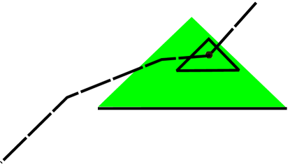
Figure 3.2: The functions $x^{\mu}$ form a wave-coordinates system on the future domain of dependence of $\widetilde{\cal{I}}_{-\eta}$, which is represented by the triangle around the dot representing $p_{1}$.

$\widetilde{\cal{I}}_{-\eta}$ satisfies (see Figure 3.2)

1. $p_{1}\in\mbox{int}{\mycal D}^{+}_{J}(\widetilde{\cal{I}}_{-\eta})$,

2. $\overline{\widetilde{\cal{I}}_{-\eta}}\subset{\mycal O}$.

Set

$${{\mycal U}}={\mycal O}\cup{\mycal D}^{+}_{J}(\widetilde{\cal{I}}_{-\eta})\;,$$

and for $p\in{{\mycal U}}$ define

$$\Psi_{{\mycal U}}(p)=\cases{\Psi_{\mycal O}(p),&$p\in{\mycal O}$,\cr q:\mbox{where $q$ is such that\ }x^{\mu}(q)=y^{\mu}(p),&$p\in{\mycal D}^{+}_{J}(\widetilde{\cal{I}}_{-\eta})\setminus{\mycal O}$.\cr}$$ (3.9)

From what has been said, (3.9) defines a $H^{s+1}_{{\mathrm{space,loc}}}$ map from ${{\mycal U}}$ to ${\mycal M}_{2}$.

Clearly ${{\mycal U}}$ is a globally hyperbolic neighborhood of $\mycal S_{1}$, and $\mycal S_{1}$ is a Cauchy surface for ${{\mycal U}}$. Note that ${\mycal O}$ is a proper subset of ${{\mycal U}}$, as $p_{1}\in{\mycal D}^{+}_{J}(\widetilde{\cal{I}}_{-\eta})$ but $p_{1}\not\in{\mycal O}$.

By construction the metric $\Psi_{{\mycal U}}^{*}g_{2}$ is of $H^{s}_{{\mathrm{space,loc}}}$-differentiability class. (This holds by hypothesis on ${\mycal O}$, since there $\Psi_{{\mycal U}}^{*}g_{2}$ coincides with $g_{1}$. This holds away from ${\mycal O}$ as well, since there the map $\Psi$ is the identity in local coordinates, and in those the metric has already been shown to be in $H^{s}_{{\mathrm{space,loc}}}$). Near $\widetilde{\cal{I}}_{-\eta}$ we have $\Psi_{{\mycal U}}^{*}g_{2}=\Psi_{*}g_{2}=g_{1}$ , thus $\Psi_{{\mycal U}}^{*}g_{2}$ coincides with $g_{1}$ there. It follows from hypothesis H2 that $\Psi_{{\mycal U}}^{*}g_{2}$ coincides with $g_{1}$ on ${{\mycal U}}\cap{\mycal D}_{J}^{+}(\widetilde{\cal{I}}_{-\eta})$. So $\Psi_{{\mycal U}}$ is a local isometry.

To prove that $\Psi_{{\mycal U}}$ is one-to-one, we proceed by contradiction, and consider $p,q\in{{\mycal U}}$, $p\neq q$, such that

$$\Psi_{{\mycal U}}(p)=\Psi_{{\mycal U}}(q)\;.$$ (3.10)

Since $\Psi_{{\mycal O}}$ is one-to-one, and since the map

$$x^{\mu}\mapsto y^{\mu}$$ (3.11)

constructed above in local coordinates is one-to-one, (3.10) can only occur with $p\neq q$ if $p$ lies in the domain of the map (3.11) and $q$ lies in ${\mycal O}$, or vice-versa. Exchanging $p$ and $q$ if necessary, we only need to consider the former case, and note that $p\not\in{\mycal O}$ since then $\Psi_{{\mycal U}}$ would coincide with $\Psi_{{\mycal O}}$ near $p$, and would therefore be injective there. So $p$ must lie in the complement of ${\mycal O}$, but $\Psi_{{\mycal U}}(p)$ must lie in $\Psi_{{\mycal O}}({\mycal O})$.

Consider a past directed timelike curve $\Gamma_{1}$ entirely contained in ${\mycal O}$, inextendible in ${\mycal O}$, and passing through $q$. Set $\Gamma:=\Psi_{\mycal O}(\Gamma_{1})$. Since the map (3.11) is a local diffeomorphism, we can invert it locally to obtain a pre-image of $\Gamma$ which is a past-directed timelike curve $\Gamma_{2}$ through $p$. Suppose that $\Gamma_{2}$ meets ${\cal{I}}_{-\epsilon}\subset{\mycal O}$ when followed to the past. Since $\Psi_{\mycal O}$ is one-to-one, the part of $\Gamma_{2}$ that lies in ${\mycal O}$ must coincide with $\Gamma_{1}$, which is not possible since $\Gamma_{1}$ has an end-point at $q$, while $\Gamma_{2}$ leaves ${\mycal O}$ through $\partial{\mycal O}$. We infer that $\Gamma_{2}$ stops before meeting ${\cal{I}}_{-\epsilon}\subset{\mycal O}$ when followed to the past. So global hyperbolicity implies that $\Gamma$ must meet $\mycal S_{1}$ when followed to the future. One can then construct a timelike curve from $\Psi_{\mycal O}(\mycal S_{1})$ to itself by following the image by $\Psi_{{\mycal U}}$ of any causal curve from $\mycal S_{1}$ to $\Psi_{\mycal O}(p)$, and then $\Gamma$ from $\Psi_{\mycal O}(p)$ to $\Psi_{{\mycal U}}$, which is not possible as we assumed that $\Psi_{{\mycal U}}$ is achronal. This shows that no distinct points $p$ and $q$ satisfying (3.10) exist, and we conclude that $\Psi_{\mycal O}$ is injective, as desired.

We have thus shown, that $({\mycal O},\Psi_{\mycal O})\leq({{\mycal U}},\Psi_{{\mycal U}})$ and $({\mycal O},\Psi_{\mycal O})\neq({{\mycal U}},\Psi_{{\mycal U}})$ which contradicts maximality of $({\mycal O},\Psi_{\mycal O})$. It follows that ${\mycal M}^{\prime}$ is Hausdorff, establishing Lemma 3.3. $\hfill\Box$

Returning to the proof of Proposition 3.2, let (${\,\,\,\,\widetilde{\!\!\!\!{\mycal M}}},\Psi$) be maximal. If ${\,\,\,\,\widetilde{\!\!\!\!{\mycal M}}}={\mycal M}_{1}$ we are done, suppose then that ${\,\,\,\,\widetilde{\!\!\!\!{\mycal M}}}\neq{\mycal M}_{1}$. Consider the topological space

$${\mycal M}^{\prime}=({\mycal M}_{1}\sqcup{\mycal M}_{2})/\Psi\;.$$

Then ${\mycal M}^{\prime}$ is Hausdorff by Lemma 3.3, hence a manifold.

We claim that ${\mycal M}^{\prime}$ is globally hyperbolic with Cauchy surface

$${\mycal S}^{\prime}=i_{{\mycal M}_{2}}({\mycal S}_{2})\approx{\mycal S}_{2}$$

(recall that $i_{{\mycal M}_{a}}$ denotes the canonical embedding of ${\mycal M}_{a}$ in ${\mycal M}^{\prime}$). Indeed, let $\Gamma^{\prime}\subset{\mycal M}^{\prime}$ be an inextendible causal curve in ${\mycal M}^{\prime}$, set

$$\Gamma_{1}=i_{{\mycal M}_{1}}^{-1}(\Gamma^{\prime}\cap i_{{\mycal M}_{1}}({\mycal M}_{1}))\;,\quad\Gamma_{2}=i_{{\mycal M}_{2}}^{-1}(\Gamma^{\prime}\cap i_{{\mycal M}_{2}}({\mycal M}_{2}))\;.$$

Clearly $\Gamma_{1}\cup\Gamma_{2}\neq\emptyset$, so that either $\Gamma_{1}\neq\emptyset$, or $\Gamma_{2}\neq\emptyset$, or both. Let the index $a$ be such that $\Gamma_{a}\neq\emptyset$. If $\hat{\Gamma}_{a}$ were an extension of $\Gamma_{a}$ in ${\mycal M}_{a}$, then $i_{{\mycal M}_{a}}(\hat{\Gamma}_{a})$ would be an extension of $\Gamma^{\prime}$ in ${\mycal M}^{\prime}$, which contradicts maximality of $\Gamma^{\prime}$, thus $\Gamma_{a}$ is inextendible. Suppose that $\Gamma_{1}\neq\emptyset$; as $\Gamma_{1}$ is inextendible in ${\mycal M}_{1}$ we must have $\Gamma_{1}\cap{\mycal S}_{1}=\{p_{1}\}$ for some $p_{1}\in{\mycal S}_{1}$. We then have $\Psi(p_{1})\in\Gamma_{2}$, so that it always holds that $\Gamma_{2}\neq\emptyset$. By global hyperbolicity of ${\mycal M}_{2}$ and inextendibility of $\Gamma_{2}$ it follows that $\Gamma_{2}\cap{\mycal S}_{2}=\{p_{2}\}$ for some $p_{2}\in{\mycal S}_{2}$, hence $\Gamma^{\prime}\cap i_{{\mycal M}_{2}}({\mycal S}_{2})=\{i_{{\mycal M}_{2}}(p_{2})\}$. This shows that $i_{{\mycal M}_{2}}({\mycal S}_{2})$ is a Cauchy surface for ${\mycal M}^{\prime}$, thus ${\mycal M}^{\prime}$ is globally hyperbolic.

As $\,\,\,\,\widetilde{\!\!\!\!{\mycal M}}\neq{\mycal M}_{1}$ we find that ${\mycal M}_{2}$ is a proper subset of ${\mycal M}^{\prime}$, which contradicts maximality of ${\mycal M}_{2}$. It follows that we must have ${\,\,\,\,\widetilde{\!\!\!\!{\mycal M}}}={\mycal M}_{1}$, and Proposition 3.2 follows. $\Box$

3.2 Proof of Theorem 1.1

We are ready now to pass to the proof of Theorem 1.1, which will occupy the remainder of this section. In view of Theorem 3.1, we need to check that conditions H1–A3, p. H1., are satisfied when $\mathbb{N}\ni s>n/2+1$.

The hypothesis H1 holds by [20], while H2 can be established using energy arguments along the lines of the proof of Lemma 2.8.

The hypothesis A0  follows from the embedding $H^{s}_{{\mathrm{space,loc}}}\subset C^{0,1}$ for $s>n/2+1$.

Condition A1 will be the contents of Proposition 3.7 where, for definiteness, the reader might want to choose the functions $F^{\mu}$ appearing in (3.12) to be zero:

Proposition 3.7.

Consider a local diffeomorphism $\Psi$ of $C^{1}$-differentiability class, and a vacuum metric $g$ of $H^{s}_{{\mathrm{space,loc}}}$-differentiability class in a coordinate system $y^{\mu}$, with $\mathbb{N}\ni s>n/2+1$. Let

$$\overline{g}:=\Psi^{*}g\;.$$

If

$$\Box_{g}y^{\mu}=F^{\mu}(g,y)\;,$$ (3.12)

for some functions $F^{\mu}$ smooth in their arguments, and if $\overline{g}$ is also of $H^{s}_{{\mathrm{space,loc}}}$-differentiability class with respect to a coordinate system $x^{\mu}$, then

$$\Psi\in H^{s+1}_{{\mathrm{space,loc}}}\;.$$ (3.13)

Proof.

Let $\mycal S_{\tau}$ denote the level sets of $x^{0}$ and let $\overline{\mycal}S_{\tau}$ denote the level sets of $y^{0}$. We start by noting that for all multi-indices $0\leq|\alpha|\leq s$ we have

$$\partial_{x}^{\alpha}g_{\mu\nu}\in L^{2}_{\textrm{\scriptsize loc}}(\overline{\mycal}S_{\tau})\;,$$ (3.14)

as needed to be able to use Proposition B.2 of Appendix B. This is clear for $0\leq|\alpha|\leq 1$ since the metric is $C^{1}$ by hypothesis. For higher derivatives, this follows from the usual higher energy estimates for the wave equation satisfied by vacuum metrics when (3.12) holds (cf., e.g., [6]), by integrating the current vector field over globally hyperbolic domains, the future boundaries of which form a covering of $\overline{\mycal}S_{\tau}$; see Remark A.3 of Appendix A.

Let ${\mycal U}_{x}$ denote the domain of definition of the coordinates $x^{\mu}$. In local coordinates so that $y^{\mu}=\Psi^{\mu}(x^{\alpha})$, (2.4)-(2.5) take the form

$$\overline{g}_{\alpha\beta}(x)=g_{\mu\nu}\left(\Psi(x)\right)\frac{\partial\Psi^{\mu}}{\partial x^{\alpha}}\frac{\partial\Psi^{\nu}}{\partial x^{\beta}}\;,$$ (3.15)

$$\frac{\partial^{2}\Psi^{\mu}}{\partial x^{\alpha}\partial x^{\beta}}=\overline{\Gamma}^{\sigma}_{\alpha\beta}(x)\frac{\partial\Psi^{\mu}}{\partial x^{\sigma}}-\Gamma^{\mu}_{\nu\rho}\left(\Psi(x)\right)\frac{\partial\Psi^{\nu}}{\partial x^{\alpha}}\frac{\partial\Psi^{\rho}}{\partial x^{\beta}}\;,$$ (3.16)

where the $\overline{\Gamma}^{\sigma}_{\alpha\beta}$’s are the Christoffel symbols of $\overline{g}$. Since both $g$ and $\overline{g}$ are in $C^{0,1}$, as in the proof of Proposition 2.6 we have $\Psi\in C^{1,1}({\mycal U}_{x})=W^{2,\infty}({\mycal U}_{x})$.

For $u<s-1-n/2$ we have $H^{s-1}_{\textrm{\scriptsize loc}}\subset C^{u}$ in dimension $n$, and a straightforward bootstrap of (3.16) shows that

$$\Psi\in C^{j_{m}}({\mycal U}_{x})\subset W^{j_{m},\infty}_{\textrm{\scriptsize loc}}({\mycal U}_{x})=W^{j_{m},\infty}_{\mathrm{space,loc}}({\mycal U}_{x})\;,$$

where $j_{m}$ is the largest integer strictly less than $s+1-\frac{n}{2}$. Let $u_{m}$ be the largest integer strictly less than $s-1-\frac{n}{2}$, thus $\Psi\in C^{u_{m}+2}$.

Suppose, first, that $u_{m}+1\neq s-1-\frac{n}{2}$. For $1\leq j\leq s-1-u_{m}$ we then have

$$H^{s-1}_{\textrm{\scriptsize loc}}\subset\cap_{1\leq j\leq s-1-u_{m}}W^{u_{m}+j,v_{j}}_{\textrm{\scriptsize loc}}\;,\ \mbox{where $v_{j}=\frac{2n}{n-2(s-1-u_{m}-j)}>2$}\;.$$ (3.17)

Suppose that

$$\Psi\in W^{u_{m}+j,v_{j-1}}_{{\mathrm{space,loc}}}\ \mbox{for some $j\in\mathbb{N}$ satisfying $2\leq j\leq s-u_{m}$.}$$ (3.18)

Since $C^{u_{m}+2}\subset W^{u_{m}+j,v_{j-1}}_{{\mathrm{space,loc}}}$, we have shown that (3.18) is true for $j=2$. One verifies that for $s>1+n/2$ Lemma B.2 applies with

$$(\ell,q)=(u_{m}+j,v_{j}) (k+1,p)=(u_{m}+j,v_{j-1})$$ and ,

establishing that the map $x\mapsto\Gamma^{\mu}_{\nu\rho}\left(\Psi(x)\right)$ is in $W^{u_{m}+j,v_{j}}_{{\mathrm{space,loc}}}$. We can thus apply Lemma B.3 with $p=v_{j-1}$, $q=v_{j}$, $k=\ell=u_{m}+j$, and $m=1$ to conclude that the map

$$x\mapsto\Gamma^{\mu}_{\nu\rho}\left(\Psi(x)\right)\frac{\partial\Psi^{\nu}}{\partial x^{\alpha}}$$

is in $W^{u_{m}+j-1,v_{j}}_{{\mathrm{space,loc}}}$. One similarly finds that the maps

$$x\mapsto\Gamma^{\mu}_{\nu\rho}\left(\Psi(x)\right)\frac{\partial\Psi^{\nu}}{\partial x^{\alpha}}\frac{\partial\Psi^{\rho}}{\partial x^{\beta}} x\mapsto\overline{\Gamma}^{\sigma}_{\alpha\beta}(x)\frac{\partial\Psi^{\mu}}{\partial x^{\sigma}}$$ and

are in $W^{u_{m}+j-1,v_{j}}_{{\mathrm{space,loc}}}$. It follows from (3.16) that $\Psi\in W^{u_{m}+j+1,v_{j}}_{{\mathrm{space,loc}}}$. In a finite number of steps one obtains (3.13). In particular the proof is complete for odd space-dimensions $n$.

For even $n$ we necessarily have $s\geq 2+n/2$, and it remains to consider the case $u_{m}+1=s-1-\frac{n}{2}$. For $1\leq j\leq s-1-u_{m}$ we then have

$$H^{s-1}_{\textrm{\scriptsize loc}}\subset\left\{\begin{array}[]{ll}\cap_{p\in[1,\infty)}W^{u_{m}+1,p}_{\textrm{\scriptsize loc}}\;,&\hbox{$u_{m}=0$;}\\ \cap_{2\leq j\leq s-1-u_{m}}W^{u_{m}+j,v_{j}}_{\textrm{\scriptsize loc}}\cap_{p\in[1,\infty)}W^{u_{m}+1,p}_{\textrm{\scriptsize loc}}\;,&\hbox{$u_{m}\geq 1$,}\end{array}\right.$$

with $v_{j}$ as in (3.17). Recall that we already know that

$$\Psi\in C^{u_{m}+2}\subset W^{u_{m}{+2},p}_{\mathrm{space,loc}}$$

for any $p\in\mathbb{R}$. We can thus choose $p$ large enough so that Lemma B.2 with $(\ell,q)=(u_{m}+2,v_{2})$, and $(k+1,p)=(u_{m}+2,p)$ applies, establishing that the map

$$x\mapsto\Gamma^{\mu}_{\nu\rho}\left(\Psi(x)\right)$$

is in $W^{u_{m}+j,v_{j}}_{{\mathrm{space,loc}}}$ with $j=2$. By Lemma B.3 with $p=q=v_{j}$, $k=\ell=u_{m}+j$, $j=2$ and $m=1$ the map

$$x\mapsto\Gamma^{\mu}_{\nu\rho}\left(\Psi(x)\right)\frac{\partial\Psi^{\nu}}{\partial x^{\alpha}}$$

is in $W^{u_{m}+j-1,v_{j}}_{{\mathrm{space,loc}}}$. One similarly finds that the maps

$$x\mapsto\overline{\Gamma}^{\sigma}_{\alpha\beta}(x)\frac{\partial\Psi^{\mu}}{\partial x^{\sigma}} x\mapsto\Gamma^{\mu}_{\nu\rho}\left(\Psi(x)\right)\frac{\partial\Psi^{\nu}}{\partial x^{\alpha}}\frac{\partial\Psi^{\rho}}{\partial x^{\beta}}$$ and

are in $W^{u_{m}+j-1,v_{j}}_{{\mathrm{space,loc}}}$ with $j=2$. It follows from (3.16) that

$$\Psi\in W^{u_{m}+j+1,v_{j}}_{{\mathrm{space,loc}}}\subset W^{u_{m}+j+1,v_{j+1}}_{{\mathrm{space,loc}}}$$

with $j=2$. One can now continue the previous induction argument to obtain (3.13). $\Box$

The hypothesis A3 follows from Proposition B.4, Appendix B.

To verify A2, near $S$ we transform the metric to a $H^{s+1}_{{\mathrm{space,loc}}}$ coordinate system where $S$ is given by the equation $\{x^{0}=0\}$. The metric is of $H^{s}_{{\mathrm{space,loc}}}$-differentiability class in this coordinate system by A3, which has already been established. We can then obtain a local solution in local coordinates by [20]. In the overlap the solutions coincide by an energy argument, as in the proof of Lemma 2.8. The globalization to the whole domain of dependence, within a single coordinate chart, is then standard.

This completes the proof of Theorem 1.1.

Appendix A Energy inequalities and Stokes theorem

In the main body of the paper we need a version of the Stokes theorem where the objects involved are poorly differentiable:

Proposition A.1.

Let $\Omega$ be a conditionally compact domain with Lipschitz boundary and let $Z$ be a vector field on an $(n+1)$-dimensional manifold ${\mycal M}$ with continuous metric $g$ and metric volume element $d\mu_{g}=\sqrt{|\det g|}d^{n+1}x$. If

$$Z\in W^{1,1}_{\textrm{\scriptsize loc}}({\mycal M})\;,\quad g\in W^{1,n}_{\textrm{\scriptsize loc}}({\mycal M})\;,$$

then the Stokes identity holds:

$$\int_{\partial\Omega}Z\rfloor d\mu_{g}=\int_{\Omega}\nabla_{\alpha}Z^{\alpha}\,d\mu_{g}\;.$$ (A.1)

Proof.

If the metric and $Z$ are Lipschitz, then (A.1) is standard (see, e.g., [15, 26, 17]). By density, it remains to show that both the left-hand side and the right-hand side are continuous in the topologies indicated.

We start with the volume integral which, in local coordinates, takes the form

$$\int\nabla_{\alpha}Z^{\alpha}d\mu_{g}=\int\left(\partial_{\alpha}Z^{\alpha}+\Gamma^{\alpha}_{\alpha\beta}Z^{\beta}\right)\sqrt{|\det g|}\,d^{n+1}x\;.$$ (A.2)

The $\partial Z$ term is clearly continuous. Concerning the $\Gamma Z$ terms, it suffices to use $\Gamma\in L^{n}_{\textrm{\scriptsize loc}}({\mycal M})$ together with the continuous Sobolev embedding $W^{1,1}_{\textrm{\scriptsize loc}}({\mycal M})\subset L^{\frac{n}{n-1}}_{\textrm{\scriptsize loc}}({\mycal M})$ to obtain the desired conclusion.

Consider, next, the boundary integral in (A.1). The result would be standard using trace theorems if $\partial\Omega$ were smooth. This is not the case, so an argument is needed: By definition of a Lipschitz hypersurface, for every $p\in\partial\Omega$ there exists local coordinates $x^{\mu}$ near $p$ in which $\partial\Omega$ takes the form

$$x^{0}=f(x^{i})\;,$$

where $f$ is Lipschitz continuous. Let new coordinates $y^{\mu}$ be defined as

$$y^{0}=x^{0}-f(x^{i})\;,\quad y^{i}=x^{i}\;.$$

Set

$$\bar{Z}^{\alpha}(y)=Z^{\alpha}(x(y))\;.$$

The map $x\to y$ is Lipschitz, with unit Jacobian wherever defined, and by the change-of-variables theorem for Lipschitz maps we find, for each $\alpha$,

$$\int\big{(}|Z^{\alpha}|+\sum_{\mu}\big{|}\partial_{x^{\mu}}Z^{\alpha}\big{|}\big{)}d^{n+1}x$$

$$=\int\big{(}|\bar{Z}^{\alpha}|+\big{|}\partial_{y^{0}}\bar{Z}^{\alpha}\big{|}+\sum_{i}\big{|}\partial_{y^{i}}\bar{Z}^{\alpha}-\frac{\partial f}{\partial x^{i}}\partial_{y^{0}}\bar{Z}^{\alpha}\big{|}\big{)}d^{n+1}y\;.$$

This implies that $\bar{Z}\in W^{1,1}_{\textrm{\scriptsize loc}}(\mathbb{R}^{n+1})$. In the coordinates $y$ the boundary $\partial\Omega$ reads $\{y^{0}=0\}$, so the usual trace theorems apply to give $\bar{Z}|_{\partial\Omega}\in W^{1/2,1}_{\textrm{\scriptsize loc}}\subset L^{1}(\partial\Omega)$. From

$$\int_{y^{0}=0}Z\rfloor d\mu_{g}=\int_{y^{0}=0}\left(\bar{Z}^{0}-\frac{\partial f}{\partial x^{i}}\bar{Z}^{i}\right)\sqrt{|\det g|}d^{n}y$$ (A.3)

one easily infers that the boundary-integral is continuous in the $W^{1,1}_{\textrm{\scriptsize loc}}({\mycal M})$ topology for $Z$ and in the topology of locally-uniform convergence for $g$. $\Box$

The following corollary of Proposition A.1 is of main interest to us:

Corollary A.2.

Suppose that $g$ is a continuous metric and assume that

$$g\in W^{1,n}_{\textrm{\scriptsize loc}}({\mycal M})\;,\quad\psi=(\psi^{A})\in H^{2}_{\textrm{\scriptsize loc}}({\mycal M})\;.$$

Then Stokes’ theorem applies to the “current vector field”

$$Z_{\mu}\equiv T_{\mu\nu}X^{\mu}:=\sum_{A}\big{(}\partial_{\mu}\psi^{A}\partial_{\nu}\psi^{A}-\frac{1}{2}g^{\sigma\rho}\partial_{\sigma}\psi^{A}\partial_{\rho}\psi^{A}g_{\mu\nu}+\psi^{A}\psi^{A}g_{\mu\nu}\big{)}X^{\mu}\;,$$ (A.4)

where $X$ is any locally Lipschitz vector field.

Proof.

We have, symbolically, $Z\approx g\psi^{2}+g^{-1}(\partial\psi)^{2}$, which is clearly in $L^{1}_{\textrm{\scriptsize loc}}({\mycal M})$. Further,

$$\partial Z\approx\partial g\psi^{2}+g\psi\partial\psi+g^{-1}\partial g(\partial\psi)^{2}+g^{-1}\partial\psi\partial^{2}\psi\;.$$

The second and last terms are obviously in $L^{1}_{\textrm{\scriptsize loc}}({\mycal M})$ for $\psi$’s which are in $H^{2}_{\textrm{\scriptsize loc}}({\mycal M})$. For the before last, we have $\partial g\in L^{n}_{\textrm{\scriptsize loc}}({\mycal M})$, while by Sobolev embedding it holds that $\partial\psi\in L^{\frac{2n}{n-1}}_{\textrm{\scriptsize loc}}({\mycal M})$, and the fact that this term is also in $L^{1}_{\textrm{\scriptsize loc}}({\mycal M})$ readily follows. The analysis of the first term is similar to that of the third. Thus the hypotheses of Proposition A.1 are satisfied.

Remark A.3.

Consider a collection of fields $\varphi^{I}$ satisfying a semi-linear system of wave-equations which, in local coordinates, take the form

$$g^{\mu\nu}\partial_{\mu}\partial_{\nu}\varphi^{I}=\chi^{I}(\partial_{\mu}\varphi^{J},\varphi^{J},x)\;,$$ (A.5)

for some functions $\chi^{I}$. For $k\geq 1$ the $k$-th energy inequality for the fields $\varphi^{I}$ can be derived using the current vector field $Z$ defined in (A.4) with

$$(\psi^{A})=\left(\frac{\partial^{j}\varphi^{I}}{\partial x^{\alpha_{1}}\cdots\partial x^{\alpha_{j}}}\right)_{0\leq j\leq k-1}\;.$$

For example, for the Einstein equations in a coordinate-gauge as in (3.12), this gives local-in-time control of the $H^{k}_{{\mathrm{space,loc}}}$ semi-norms of the metric by taking $(\varphi^{I})=(g_{\mu\nu})$.

Appendix B Manifolds of $W^{k+1,p}_{\mathrm{space,loc}}$ differentiability class

When using wave-coordinates for a $H^{s}_{{\mathrm{space,loc}}}$ metric one needs to work with coordinate transformations which are not smooth but of $H^{s+1}_{{\mathrm{space,loc}}}$ differentiability class. This begs the question, what happens with functions and tensor fields under such coordinate changes. This is the main issue addressed in this appendix.

Consider a smooth manifold ${\mycal M}$; on such a manifold one can define in an invariant way tensor fields which are of $C^{\infty}$ differentiability class, similarly for $C^{k}$, $W^{k,p}_{\textrm{\scriptsize loc}}$, or $W^{k,p}_{\mathrm{space,loc}}$ class. For example, one says that a tensor field is of $W^{k,p}_{\mathrm{space,loc}}$ class if there exists a covering of ${\mycal M}$ by coordinate patches such that the coordinate components of the tensor in question are in $W^{k,p}_{\mathrm{space,loc}}$ in each of the coordinate patches. Now, even though the transition functions when going from one coordinate system to another are smooth, it is not clear that $W^{k,p}_{\mathrm{space,loc}}$-differentiability will be true in all coordinate system, because the integral differentiability conditions might fail to hold on the constant-$x^{0}$-slices of some smooth coordinate systems, unless some preferred coordinate $x^{0}$ has been chosen. To address this issue for the metric tensor, we will assume for definiteness wave coordinates and vacuum field equations. In fact, the invariance of the $W^{k,p}_{\mathrm{space,loc}}$-differentiability conditions holds for any tensor field satisfying wave-type equations, and many alternative coordinate-conditions for vacuum metrics are possible as e.g. in (3.12). Note that this problem does not arise for $C^{\infty}$, $C^{k}$, or $W^{k,p}_{\textrm{\scriptsize loc}}$ tensor fields.

Let us start with a definition:

Definition B.1.

Let $k\in\mathbb{R}$, $p\in[1,\infty]$. A function $f$ will be said to be of $W^{k,p}_{\mathrm{space,loc}}$-differentiability class if every point $p\in{\mycal M}$ has a coordinate neighborhood ${\mycal U}=I\times{\mycal V}$, where $I$ is the range of a coordinate $t\equiv x^{0}$, with the following properties: On every level set $\mycal S_{\tau}\subset{\mycal U}$ of the coordinate $t$ we have $f\in W^{k,p}_{\textrm{\scriptsize loc}}(\mycal S_{\tau})$, with the time-derivatives of order $0\leq\ell\leq k$ of $f$ being of $W^{k-\ell,p}_{\mathrm{space,loc}}$ differentiability. Furthermore the functions

$$I\ni t\mapsto\|\partial^{\ell}_{t}f|_{\mycal S_{t}}\|_{W^{k-\ell,p}}\;,\qquad 0\leq\ell\leq k$$

are required to be continuous.

We set $H^{k}_{{\mathrm{space,loc}}}:=W^{k,2}_{\mathrm{space,loc}}$.

To continue, it is convenient to introduce the following notation: for $x,y\in\mathbb{R}\cup\{\infty\}$, we will write $x>_{\!\!*}y$ if the following holds:

$$x>_{\!\!*}y\Longleftrightarrow\cases{x\geq y\ ,&if $y>0$\ ,\cr x>y\ ,&if $y\leq 0$\ .}$$ (B.1)

(Note that for $x\geq 0$ the only value of $x$ at which “$>_{\!\!*}$” does not coincide with “$\geq$” is $x=0$.) In this notation the Sobolev embedding theorem, in dimension $n$, can be stated as [1, 3]:

$$W^{s,t}_{\mathrm{space,loc}}\subset W^{u,v}_{\mathrm{space,loc}}\quad\Longleftrightarrow\quad u\leq s\ \mbox{ and }\ \frac{1}{v}>_{\!\!*}\frac{1}{t}-\frac{s-u}{n}\ \;.$$ (B.2)

We have the following:

Lemma B.2.

Let $\Omega$ and ${\cal U}$ be open subsets of $\mathbb{R}^{n+1}$, and let $\Psi:\Omega\to{\cal U}$ be a $C^{1}$ diffeomorphism such that $\Psi\in W^{k+1,p}_{{\mathrm{space,loc}}}(\Omega;{\bar{R}}^{n})$ (with respect to the coordinate $x^{0}$), with $p\in[1,\infty]$, $k\in\mathbb{N}$, $kp>n$. Write $\Psi=\big{(}\Psi^{0}(x^{0},x^{k}),\Psi^{\ell}(x^{0},x^{k})\big{)}$, and let $\overline{\mycal}S_{\tau}$ denote the level sets of $\Psi^{0}$, assume that $\partial_{0}\Psi^{0}$ has no zeros so that the $\overline{\mycal}S_{\tau}$ are graphs which can be parametrized by $x^{i}$. Let $(\ell,q)$ be such that the $n$-dimensional Sobolev embedding $W^{k+1,p}_{{\mathrm{space,loc}}}\subset W^{\ell,q}_{\textrm{\scriptsize loc}}$ holds. If for every $\tau$ such that $\overline{\mycal}S_{\tau}\neq\emptyset$, for every compact $K$ satisfying $K\subset\overline{\mycal}S_{\tau}$, and for every $0\leq j\leq\ell$ we have

$$\int_{K}\bigg{|}\frac{\partial^{j}F}{\partial x^{\alpha_{1}}\cdots\partial x^{\alpha_{j}}}\bigg{|}^{q}d^{n}x<\infty\;,$$ (B.3)

then

$$F\circ\Psi\in W^{\ell,q}_{{\mathrm{space,loc}}}(\Omega)\ .$$

Proof.

The proof is a straightforward adaptation of that of Lemma A.2 in [4]. $\Box$

We also need:

Lemma B.3.

Let $0\leq m\leq\ell\leq k$, $q,p\in[1,\infty]$, $kp>n$. Suppose that $(\ell,q)$ is such that the $n$-dimensional Sobolev embedding $W^{k,p}_{{\mathrm{space,loc}}}\subset W^{\ell,q}_{\mathrm{space,loc}}$ holds. Then the product map

$$W^{k-m,p}_{{\mathrm{space,loc}}}\times W^{\ell,q}_{{\mathrm{space,loc}}}\ \ni\ (f,g)\ \longrightarrow fg\in W^{\ell-m,q}_{{\mathrm{space,loc}}}$$

is continuous.

Proof.

The proof is a repetition of that of Lemma A.4 in [4]. $\Box$

Finally:

Proposition B.4.

Under the conditions of Lemma B.2, let $F$ be a tensor field the cooordinate-components of which satisfy (B.3). If moreover the $n$-dimensional Sobolev embedding

$$W^{k,p}_{{\mathrm{space,loc}}}\subset W^{\ell,q}_{\mathrm{space,loc}}$$

holds, then $\Psi^{*}F\in W^{\ell,q}_{\mathrm{space,loc}}$.

Proof.

This follows from Lemmata B.2-B.3, as in [4, Appendix A]. $\Box$

References

- [1] R.A. Adams, Sobolev spaces, Academic Press, N.Y., 1975.
- [2] S. Alinhac and P. Gérard, Opérateurs pseudo-différentiels et théorème de Nash-Moser, Savoirs Actuels. [Current Scholarship], InterEditions, Paris, 1991.
- [3] T. Aubin, Nonlinear analysis on manifolds. Monge–Ampère equations, Springer, New York, Heidelberg, Berlin, 1982.
- [4] R. Bartnik and P.T. Chruściel, Boundary value problems for Dirac-type equations, (2003), arXiv:math.DG/0307278.
- [5] Y. Choquet-Bruhat, Einstein constraints on -dimensional compact manifolds, Class. Quantum Grav. 21 (2004), S127–S152, arXiv:gr-qc/0311029; in “A spacetime safari: essays in honour of Vincent Moncrief”. MR 2053003 (2005g:83011)
- [6] , General relativity and the Einstein equations, Oxford Mathematical Monographs, Oxford University Press, Oxford, 2009. MR MR2473363 (2010f:83001)
- [7] Y. Choquet-Bruhat and R. Geroch, Global aspects of the Cauchy problem in general relativity, Commun. Math. Phys. 14 (1969), 329–335. MR MR0250640 (40 #3872)
- [8] Y. Choquet-Bruhat and J. York, The Cauchy problem, General Relativity (A. Held, ed.), Plenum Press, New York, 1980, pp. 99–172. MR 583716 (82k:58028)
- [9] P.T. Chruściel, On completeness of orbits of Killing vector fields, Class. Quantum Grav. 10 (1993), 2091–2101, arXiv:gr-qc/9304029.
- [10] , Uniqueness of black holes revisited, Helv. Phys. Acta 69 (1996), 529–552, Proceedings of Journées Relativistes 96 (N. Straumann, Ph. Jetzer and G. Lavrelashvili, eds), arXiv:gr-qc/9610010.
- [11] , Elements of causality theory, (2011), arXiv:1110.6706v1 [gr-qc].
- [12] P.T. Chruściel, G.J. Galloway, and D. Pollack, Mathematical general relativity: a sampler, Bull. Amer. Math. Soc. (N.S.) 47 (2010), 567–638, arXiv:1004.1016 [gr-qc]. MR 2721040 (2011j:53152)
- [13] P.T. Chruściel and J. Grant, On Lorentzian causality with continuous metrics, Class. Quantum Grav. 29 (2012), 145001, arXiv:1110.0400v2 [gr-qc].
- [14] P.T. Chruściel and D.B. Singleton, Nonsmoothness of event horizons of Robinson-Trautman black holes, Commun. Math. Phys. 147 (1992), 137–162. MR 1171763 (93i:83059)
- [15] B.K. Driver, Analysis, http://www.math.ucsd.edu/~bdriver/231-02-03/Lecture_Notes/PDE-Anal-Book/analpde1.pdf.
- [16] A. Fathi and A. Siconolfi, On smooth time functions, Math. Proc. Camb. Phil. Soc. 152 (2012), 303–339.
- [17] H. Federer, Geometric measure theory, Springer Verlag, New York, 1969, (Die Grundlehren der mathematischen Wissenschaften, Vol. 153).
- [18] Y. Fourès-Bruhat, Théorème d’existence pour certains systèmes d’équations aux dérivées partielles non linéaires, Acta Math. 88 (1952), 141–225.
- [19] S.W. Hawking and G.F.R. Ellis, The large scale structure of space-time, Cambridge University Press, Cambridge, 1973, Cambridge Monographs on Mathematical Physics, No. 1. MR MR0424186 (54 #12154)
- [20] T.J.R. Hughes, T. Kato, and J.E. Marsden, Well-posed quasi-linear second-order hyperbolic systems with applications to nonlinear elastodynamics and general relativity, Arch. Rat. Mech. Anal. 63 (1977), 273–294.
- [21] J.L. Kelley, General topology, Springer-Verlag, New York, 1975, Reprint of the 1955 edition [Van Nostrand, Toronto, Ont.], Graduate Texts in Mathematics, No. 27.
- [22] S. Klainerman and I. Rodnianski, Ricci defects of microlocalized Einstein metrics, Jour. Hyperbolic Diff. Equ. 1 (2004), 85–113. MR MR2052472 (2005f:58048)
- [23] , The causal structure of microlocalized rough Einstein metrics, Ann. of Math. (2) 161 (2005), 1195–1243. MR MR2180401 (2007d:58052)
- [24] , Rough solutions of the Einstein-vacuum equations, Ann. of Math. (2) 161 (2005), 1143–1193. MR MR2180400 (2007d:58051)
- [25] S. Klainerman, I. Rodnianski, and J. Szeftel, Overview of the proof of the Bounded Curvature Conjecture, (2012), arXiv:1204.1772 [gr-qc].
- [26] P. Mattila, Geometry of sets and measures in Euclidean spaces, Cambridge Studies in Advanced Mathematics, vol. 44, Cambridge University Press, Cambridge, 1995, Fractals and rectifiability.
- [27] D. Maxwell, Rough solutions of the Einstein constraint equations, J. Reine Angew. Math. 590 (2006), 1–29, arXiv:gr-qc/0405088. MR MR2208126 (2006j:58044)
- [28] G. Métivier, Para-differential calculus and applications to the Cauchy problem for nonlinear systems, Centro di Ricerca Matematica Ennio De Giorgi (CRM) Series, vol. 5, Edizioni della Normale, Pisa, 2008, http://www.math.u-bordeaux1.fr/~metivier/Total.Mai08v2.pdf.
- [29] D. Parlongue, Geometric uniqueness for non-vacuum Einstein equations and applications, arXiv:1109.0644 [math-ph].
- [30] F. Planchon and I. Rodnianski, On uniqueness for the Cauchy problem in general relativity, (2007), in preparation.
- [31] H. Ringström, The Cauchy problem in general relativity, ESI Lectures in Mathematics and Physics, European Mathematical Society (EMS), Zürich, 2009. MR 2527641 (2010j:83001)
- [32] H. Smith and D. Tataru, Sharp local well-posedness results for the nonlinear wave equation, Ann. of Math. (2) 162 (2005), 291–366. MR MR2178963 (2006k:35193)
- [33] Q. Wang, Rough solutions of Einstein vacuum equations in CMCSH gauge, (2012), arXiv:1201.0049 [math.AP].
- [34] H. Whitney, Differentiable manifolds, Ann. of Math. (2) 37 (1936), 645–680.