Residual, restarting and Richardson iteration
for the matrix exponential, revised

Abstract

A well-known problem in computing some matrix functions iteratively is the lack of a clear, commonly accepted residual notion. An important matrix function for which this is the case is the matrix exponential. Suppose the matrix exponential of a given matrix times a given vector has to be computed. We develop the approach of Druskin, Greenbaum and Knizhnerman (1998) and interpret the sought-after vector as the value of a vector function satisfying the linear system of ordinary differential equations (ODE) whose coefficients form the given matrix. The residual is then defined with respect to the initial-value problem for this ODE system. The residual introduced in this way can be seen as a backward error. We show how the residual can be computed efficiently within several iterative methods for the matrix exponential. This completely resolves the question of reliable stopping criteria for these methods. Further, we show that the residual concept can be used to construct new residual-based iterative methods. In particular, a variant of the Richardson method for the new residual appears to provide an efficient way to restart Krylov subspace methods for evaluating the matrix exponential.

To the memory of my father

1 Introduction

Matrix functions, and particularly the matrix exponential, have been an important tool in scientific computations for decades (see e.g. [12, 13, 15, 10, 16]). The lack of a clear notion for a residual for many matrix functions has been a known problem in iterative computation of matrix functions [2, 10, 37]. Although it is possible to define a residual for some matrix functions such as the inverse or the square root, for many important matrix functions including the matrix exponential, sine and cosine, no natural notion for residuals seems to exist.

Assume for given $A\in\mathbb{R}^{n\times n}$, such that $A+A^{*}$ is positive semidefinite, and $v\in\mathbb{R}^{n}$ the vector

$$y=\exp(-A)v$$ (1)

has to be computed. The question is how to evaluate the quality of an approximate solution

$$y_{k}\approx\exp(-A)v,$$ (2)

where $k$ refers to the number of steps (iterations) needed to construct $y_{k}$. We interpret the vector $y$ as the value of a vector function $y(t)$ at $t=1$ such that

$$y^{\prime}(t)=-Ay(t),\quad y(0)=v.$$ (3)

The exact solution of this initial-value problem (IVP) is given by

$$y(t)=\exp(-tA)v.$$

Assuming now that there is a vector function $y_{k}(t)$ such that $y_{k}(1)=y_{k}$, we define the residual for $y_{k}(t)\approx y(t)$ as

$$r_{k}(t)\equiv-Ay_{k}(t)-y_{k}^{\prime}(t).$$ (4)

The key point in this residual concept is that $y=\exp(-A)v$ is seen not as a problem on its own but rather as the exact solution formula for the problem (3). The latter provides the equation where the approximate solution is substituted to yield the residual. We illustrate this in Table 1, where the introduced matrix exponential residual is compared against the conventional residual for a linear system $Ay=v$. As can be seen in the Table, the approximate solution satisfies a perturbed IVP, where the perturbation is the residual. Thus, the introduced residual can be seen as a backward error (see Section 4 for residual-based error estimates). If one is interested in computing the matrix exponential $\exp(-A)$ itself, then the residual can be defined with respect to the matrix IVP

$$X^{\prime}(t)=-AX(t),\quad X(0)=I,$$

with the exact solution $X(t)=\exp(-tA)$. Checking the norm of $r_{k}(t)$ in (4) is proposed as a possible stopping criterion of Krylov subspace iterations first in [4] and more recently for a similar matrix function in [22].

Table 1: The linear system and matrix exponential residuals. In both cases the sought-after vector is $f(A)v$, with either $f(x)=1/x$ or $f(x)=\exp(-x)$. The error is defined as the exact solution minus the approximate solution.

$f(x)$	$1/x$		$\exp(-x)$
exact solution $y$	$y=A^{-1}v$		$\begin{aligned} &\text{define }y(t)=\exp(-tA)v,\\ &\text{set }y:=y(1)\end{aligned}$
residual equation	$Ay=v$		$\left\{\begin{aligned} y^{\prime}(t)&=-Ay(t)\\ y(0)&=v\end{aligned}\right.$
residual for $y_{k}\approx y$	$r_{k}=v-Ay_{k}$		$r_{k}(t)=-Ay_{k}(t)-y_{k}^{\prime}(t)$
mapping error $\epsilon_{k}$ $\rightarrow$ residual $r_{k}$	$r_{k}=A\epsilon_{k}$		$\left\{\begin{aligned} r_{k}(t)&=\epsilon^{\prime}_{k}(t)+A\epsilon_{k}(t)\\ \epsilon_{k}(0)&=0\end{aligned}\right.$
perturbed problem (backward stability)	$Ay_{k}=v-r_{k}$		$\left\{\begin{aligned} y^{\prime}_{k}(t)&=-Ay_{k}(t)-r_{k}(t)\\ y_{k}(0)&=v\end{aligned}\right.$

The contribution of this paper is twofold. First, it turns out that the residual (4) can be efficiently computed within several iterative methods for matrix exponential evaluation. We show how this can be done in several popular Krylov subspace and Chebyshev polynomial methods for computing $\exp(-A)v$. Second, we show how the residual notion leads to new algorithms to compute the matrix exponential. Two basic Richardson-like iterations are proposed and discussed. When combined with Krylov subspace methods, one of them can be seen as an efficient way to restart the Krylov subspace methods. Furthermore, this approach for the matrix exponential residual can be readily extended to the sine and cosine matrix functions (see the conclusion section).

The equivalence between problems (2) and (3) has been widely used in numerical literature and computations. In addition to already cited work [4, 22] see e.g. the very first formula in [27] or [15, Section 10.1]. Moreover, methods for solving (2) are applied to (3) (for instance, exponential time integrators [18, 19]) and vice versa [27, Section 4]. In [37], van den Eshof and Hochbruck represent the error $\epsilon_{k}(t)\equiv y(t)-y_{k}(t)$ as the solution of the IVP $\epsilon_{k}^{\prime}(t)=-A\epsilon_{k}(t)+r_{k}(t)$, $\epsilon_{k}(0)=0$ and obtain an explicit, non-computable expression for $\epsilon_{k}(t)$. This allows them to justify a stopping criterion for their shift-and-invert Lanczos algorithm, based on stagnation of the approximations. Although being used, especially in the field of numerical ODEs (see e.g. [9, 33, 25, 21]), the exponential residual (4) does seem to have a potential which has not been fully exploited yet, in particular in matrix computations. Our paper aims at filling this gap.

The paper is organized as follows. Section 2 is devoted to the matrix exponential residual within Krylov subspace methods. In Section 3 we show how the Chebyshev iterations can be modified to adopt the residual control. Section 4 presents some simple residual-based error estimates. Richardson iteration for the matrix exponential is the topic of Section 5. Numerical experiments are discussed in Section 6, and conclusions are drawn in the last section.

Throughout the paper, unless noted otherwise, $\|\cdot\|$ denotes the Euclidean vector 2-norm or the corresponding induced matrix norm.

2 Matrix exponential residual in Krylov subspace methods

Krylov subspace methods have become an important tool for computing matrix functions (see e.g. [38, 5, 23, 11, 31, 6, 17, 7, 18]). For $A\in\mathbb{R}^{n\times n}$ and $v\in\mathbb{R}^{n}$ given, the Arnoldi process yields, after $k$ steps, vectors $v_{1}$, …, $v_{k+1}\in\mathbb{R}^{n}$ that are orthonormal in exact arithmetic and span the Krylov subspace $\mathcal{K}_{k}(v,Av,\dots,A^{k-1}v)$ (see e.g. [13, 32, 39]). If $A=A^{*}$, the Lanczos process is usually used instead of Arnoldi. Together with the basis vectors $v_{j}$, the Arnoldi or Lanczos processes deliver an upper-Hessenberg matrix $\underline{H}_{k}\in\mathbb{R}^{(k+1)\times k}$, such that the following relation holds [13, 32, 39]:

$$AV_{k} =V_{k+1}\underline{H}_{k},\quad\text{or equivalently,}$$ (5)

$$AV_{k} =V_{k}H_{k}+h_{k+1,k}v_{k+1}e_{k}^{T},$$

where $V_{k}\in\mathbb{R}^{n\times k}$ has columns $v_{1}$, …, $v_{k}$, $H_{k}\in\mathbb{R}^{k\times k}$ is the matrix $\underline{H}_{k}$ without the last row $(0,\cdots,0,h_{k+1,k})$, and $e_{k}=(0,\cdots,0,1)^{T}\in\mathbb{R}^{k}$. The first basis vector $v_{1}$ is the normalized vector $v$: $v_{1}=v/\|v\|$.

2.1 Ritz-Galerkin approximation

An approximation $y_{k}$ to the matrix exponential $y=\exp(-A)v$ is usually computed as $y_{k}(1)$, with

$$y_{k}(t)=V_{k}\exp(-tH_{k})(\beta e_{1}),$$ (6)

where $\beta=\|v\|$ and $e_{1}=(1,0,\dots,0)^{T}\in\mathbb{R}^{k}$. An important property of the Krylov subspace is its scaling invariance: application of the Arnoldi process to $tA$, $t\in\mathbb{R}$, results in the upper-Hessenberg matrix $t\underline{H}_{k}$, and the basis vectors $v_{1}$, …, $v_{k+1}$ are independent of $t$. It is convenient for us to write

$$y_{k}(t)=V_{k}u_{k}(t),\quad u_{k}(t)\equiv\exp(-tH_{k})(\beta e_{1}),$$ (6^′)

with $u_{k}(t):\mathbb{R}\rightarrow\mathbb{R}^{k}$ being the solution of the projected IVP

$$u_{k}^{\prime}(t)=-H_{k}u_{k}(t),\quad u_{k}(0)=\beta e_{1}.$$ (7)

The following simple Lemma (cf. [4, formula (29)]) provides an explicit expression for the residual.

Lemma 1.

Let $y_{k}(t)\approx y(t)=\exp(-tA)v$ be the Krylov subspace approximation given by (6). Then for any $t\geqslant 0$ the residual $r_{k}(t)$ for $y_{k}(t)\approx y(t)$ is

$$r_{k}(t) =-\beta h_{k+1,k}e_{k}^{T}\exp(-tH_{k})e_{1}v_{k+1},$$

$$\|r_{k}(t)\| =|\beta h_{k+1,k}e_{k}^{T}\exp(-tH_{k})e_{1}|=|h_{k+1,k}[u_{k}(t)]_{k}|,$$

where $[u_{k}(t)]_{k}$ is the last entry of the vector function $u_{k}(t)$ defined in (6^′).

Proof.

It follows from (6) that $y_{k}^{\prime}(t)=-V_{k}H_{k}\exp(-tH_{k})(\beta e_{1})$. From the Arnoldi relation (5) we have

$$Ay_{k}(t)=AV_{k}\exp(-tH_{k})(\beta e_{1})=(V_{k}H_{k}+h_{k+1,k}v_{k+1}e_{k}^{T})\exp(-tH_{k})(\beta e_{1}),$$

which yields the result:

$$r_{k}(t)=-Ay_{k}(t)-y_{k}^{\prime}(t)=-h_{k+1,k}v_{k+1}e_{k}^{T}\exp(-tH_{k})(\beta e_{1}).$$

∎

Note that the Krylov subspace approximation (6) satisfies the initial condition $y_{k}(0)=v$ by construction:

$$y_{k}(0)=V_{k}(\beta e_{1})=\beta v_{1}=v.$$

Thus, there is no danger that the residual $r_{k}(t)=-Ay_{k}(t)-y_{k}^{\prime}(t)$ is small in norm for some $y_{k}(t)$ approaching a solution of the ODE system $y^{\prime}=Ay$ with other initial data.

The residual notion (4) allows us to see (6) as the Ritz-Galerkin approximation: the residual vector $r_{k}(t)$ is orthogonal, for any $t\geqslant 0$, to the search space $\mathrm{span}(v_{1},\dots,v_{k})$:

$$V_{k}^{*}r_{k}(t)=V_{k}^{*}(-Ay_{k}(t)-y_{k}^{\prime}(t))=V_{k}^{*}(-AV_{k}u_{k}(t)-V_{k}u_{k}^{\prime}(t))=-H_{k}u_{k}(t)-u_{k}^{\prime}(t)=0.$$ (8)

Here we used the relation $V_{k}^{*}AV_{k}=H_{k}$, which follows from (5) if $V_{k}$ is orthonormal (this may not always be the case in floating point arithmetic).

The residual $r_{k}(t)$ turns out to be closely related to the so-called generalized residual $\rho_{k}(t)$ [18]. Following [18] (see also [31]), we can write

$$y_{k}(t) =\beta V_{k}\exp(-tH_{k})e_{1} =\frac{1}{2\pi i}\oint_{\Gamma}e^{\lambda}V_{k}(\lambda I+tH_{k})^{-1}\beta e_{1}\mathrm{d}\lambda,$$

$$y(t) =\exp(-tA)v =\frac{1}{2\pi i}\oint_{\Gamma}e^{\lambda}(\lambda I+tA)^{-1}v\mathrm{d}\lambda,$$

where $\Gamma$ is a closed contour in $\mathbb{C}$ encircling the spectrum of $A$. Thus, $y_{k}(t)$ is an approximation to $y(t)$ where the resolvent inverse $(\lambda I+tA)^{-1}v$ is approximated by $k$ steps of the fully orthogonal method (FOM):

$$\epsilon_{k}=y(t)-y_{k}(t)=\frac{1}{2\pi i}\oint_{\Gamma}e^{\lambda}\mathrm{error}_{k}^{\mathrm{FOM}}\mathrm{d}\lambda.$$

Since the FOM error is unknown, the authors of [18] replace it by the known FOM residual, which is $\beta(-th_{k+1,k})v_{k+1}e_{k}^{T}(\lambda I+tH_{k})^{-1}e_{1}$. This leads to the generalized residual

$$\rho_{k}(t) \equiv\frac{1}{2\pi i}\oint_{\Gamma}e^{\lambda}\beta(-th_{k+1,k})v_{k+1}e_{k}^{T}(\lambda I+tH_{k})^{-1}e_{1}\mathrm{d}\lambda$$ (9)

$$=-\beta th_{k+1,k}e_{k}^{T}\exp(-tH_{k})e_{1}\,v_{k+1},$$

which coincides, up to a factor $t$, with our matrix exponential residual $r_{k}(t)$. For the generalized residual, this provides a justification which is otherwise lacking: strictly speaking, there is no reason why the error in the integral expression above can be replaced by the residual. In Section 6.4, a numerical test is presented to compare stopping criteria based on $r_{k}(t)$ and $\rho_{k}(t)$.

2.2 Shift-and-invert Arnoldi/Lanczos approximations

In the shift-and-invert (SaI) Arnoldi/Lanczos approximations [28, 37] the Krylov subspace is built up with respect to the matrix $(I+\gamma A)^{-1}$, with $\gamma>0$ being a parameter, so that the Krylov basis matrix $V_{k+1}\in\mathbb{R}^{n\times(k+1)}$ and an upper-Hessenberg matrix $\underline{\tilde{H}}_{k}\in\mathbb{R}^{(k+1)\times k}$ are built such that (cf. (5))

$$(I+\gamma A)^{-1}V_{k} =V_{k+1}\underline{\tilde{H}}_{k},\quad\text{or, equivalently,}$$ (10)

$$(I+\gamma A)^{-1}V_{k} =V_{k}\tilde{H}_{k}+\tilde{h}_{k+1,k}v_{k+1}e_{k}^{T},$$

where $\tilde{H}_{k}\in\mathbb{R}^{k\times k}$ is the first $k$ rows of $\underline{\tilde{H}}_{k}$. The approximation $y_{k}(t)\approx\exp(-tA)v$ is then computed as given by (6), with $H_{k}$ defined as [37]

$$H_{k}=\frac{1}{\gamma}(\tilde{H}_{k}^{-1}-I).$$ (11)

Relation (10) can be rewritten as (cf. formula (4.1) in [37])

$$AV_{k}=V_{k}H_{k}-\frac{\tilde{h}_{k+1,k}}{\gamma}(I+\gamma A)v_{k+1}e_{k}^{T}\tilde{H}_{k}^{-1},$$ (12)

which leads to the following lemma.

Lemma 2.

Let $y_{k}(t)\approx y(t)=\exp(-tA)v$ be the SaI Krylov subspace approximation (6), with $H_{k}$ defined in (11). Then for any $t\geqslant 0$ the residual $r_{k}(t)$ for $y_{k}(t)\approx y(t)$ is

$$r_{k}(t) =\beta\,\frac{\tilde{h}_{k+1,k}}{\gamma}\,e_{k}^{T}\tilde{H}_{k}^{-1}\exp(-tH_{k})e_{1}(I+\gamma A)v_{k+1},$$

$$\|r_{k}(t)\| \leqslant\beta\left|\frac{\tilde{h}_{k+1,k}}{\gamma}\right||e_{k}^{T}\tilde{H}_{k}^{-1}\exp(-tH_{k})e_{1}|(1+\gamma\|A\|).$$

Proof.

The proof is very similar to that of Lemma 1. Instead of the conventional Arnoldi relation (5), relation (12) should be used. ∎

2.3 Error estimation in Krylov subspace methods

If $y_{k}(t)$ is a Krylov subspace approximation to $y(t)=\exp(-tA)v$, the error function $\epsilon_{k}(t)\equiv y(t)-y_{k}(t)$ satisfies the IVP

$$\epsilon_{k}^{\prime}(t)=-A\epsilon_{k}(t)+r_{k}(t),\quad\epsilon_{k}(0)=0.$$ (13)

To estimate the error, this equation can be solved approximately by any suitable time integration scheme; for example, by Krylov exponential schemes as discussed e.g. in [11, Section 4] or [18]. The time integration process for solving (13) can further be optimized to take into account that the residual function $r_{k}(t)$ depends on time as $r_{k}(t)=\psi_{k}(t)v_{k+1}$ with $v_{k+1}=\mathop{\operator@font const}\nolimits$ and $\psi_{k}(t)$ being a scalar function of $t$ (see Lemma 1):

$$\psi_{k}(t)\equiv-\beta h_{k+1,k}e_{k}^{T}\exp(-tH_{k})e_{1}.$$

Van den Eshof and Hochbruck [37] propose to get an error estimate by replacing in $\epsilon_{k}(t)\equiv y(t)-y_{k}(t)$ the exact solution $y(t)$ with the same continued Krylov process approximation $y_{k+m}(t)$:

$$\epsilon_{k}(t) \approx y_{k+m}(t)-y_{k}(t)=V_{k+m}u_{k+m}(t)-V_{k}u_{k}(t)=V_{k+m}\tilde{\epsilon}_{k}(t),$$ (14)

$$\|\epsilon_{k}(t)\| \approx\|\tilde{\epsilon}_{k}(t)\|=\|u_{k+m}(t)-\tilde{u}_{k}(t)\|,$$

where

$$V_{k}u_{k}(t)=V_{k+m}\tilde{u}_{k}(t),\quad\tilde{u}_{k}(t)=[\,(u_{k}(t))^{T},\underbrace{0,\dots,0}_{m}\,]^{T}$$

and $u_{k}(t)$ and $u_{k+m}(t)$ are the solutions of the projected IVP (7) obtained with respectively $k$ and $k+m$ Krylov steps. It is not difficult to see that in this case $\tilde{\epsilon}_{k}(t)\equiv u_{k+m}(t)-\tilde{u}_{k}(t)$ is the Galerkin solution of (13) with respect to the subspace $\mathrm{colspan}V_{k+m}$. Indeed, we have

$$y^{\prime}_{k+m} =-Ay_{k+m}-r_{k+m}(t),\quad y_{k+m}(t) =V_{k+m}u_{k+m}(t),$$

$$y^{\prime}_{k} =-Ay_{k}-r_{k}(t),\quad y_{k}(t) =V_{k+m}\tilde{u}_{k}(t).$$

Subtracting $y_{k}^{\prime}$ from $y_{k+m}^{\prime}$ and multiplying the result from the left by $V_{k+m}^{*}$ (in assumption the orthonormality of $V_{k+m}$ is not spoiled in floating point arithmetic) we obtain

$$(u_{k+m}(t)-\tilde{u}_{k}(t))^{\prime}=-H_{k+m}(u_{k+m}(t)-\tilde{u}_{k}(t))+V_{k+m}^{*}r_{k}(t),\quad V_{k+m}^{*}r_{k}(t)=\psi_{k}(t)e_{k+1},$$

and we arrive at the projected IVP

$$\tilde{\epsilon}_{k}^{\prime}(t)=-H_{k+m}\tilde{\epsilon}_{k}(t)+\psi_{k}(t)e_{k+1},$$ (15)

where $e_{k+1}$ is the $(k+1)$th basis vector in $\mathbb{R}^{k+m}$. This shows that error estimation by the same continued Krylov process is a better option than solving the correction equation (13) by a new Krylov process: the latter would mean that we neglect the built up subspace. In fact, solving IVP (13) by another process and then correcting the approximate solution $y_{k}(t)$ can be seen as a restarting of the Krylov subspace. We explore this approach further in Section 5.

3 Matrix exponential residual for Chebyshev approximations

A well-known method to compute $y_{m}(t)\approx\exp(-tA)v$ is based on the Chebyshev polynomial expansion (see for instance [35, 30]):

$$y_{m}(t)=P_{m}(-tA)v=\left[\sum_{k=1}^{m}c_{k}T_{k}(-tA)+\frac{c_{0}}{2}I\right]v.$$ (16)

Here we assume that the matrix $tA$ can be transformed to have its eigenvalues within the interval $[-1,1]\subset\mathbb{R}$ (for example, $A$ can be a Hermitian or a skew-Hermitian matrix). Here, $T_{k}$ are the Chebyshev polynomials of the first kind, whose actions on the given vector $v$ can be computed by the Chebyshev recursion

$$T_{0}(x)=1,\quad T_{1}(x)=x,\quad T_{k+1}(x)=2xT_{k}(x)-T_{k-1}(x),\quad k=1,2,\dots,$$ (17)

and the coefficients $c_{k}$ can be computed, for a large $M$, as

$$c_{k}=\frac{2}{M}\sum_{j=1}^{M}\exp(\cos(\theta_{j}))\cos(k\theta_{j}),\quad k=0,1,\dots,m,\quad\theta_{j}=\frac{\pi(j-\frac{1}{2})}{M},$$ (18)

which means interpolating $\exp(x)$ at the Chebyshev polynomial roots (see e.g. [30, Section 3.2.3]). This Chebyshev polynomial approximation is used for evaluating different matrix functions in [2].

The recursive algorithm (16)–(18) can be modified to provide, along with $y_{m}(t)$, vectors $y_{m}^{\prime}(t)$ and $Ay_{m}(t)$, so that the exponential residual $r_{m}(t)\equiv-Ay_{m}(t)-y_{m}^{\prime}(t)$ can be controlled in the course of the iterations. To do this, we use the well-known relations

$$T_{k}^{\prime}(x) =kU_{k-1}(x),$$ (19)

$$xT_{k}(x) =\frac{1}{2}(T_{k+1}(x)+T_{k-1}(x)),$$ (20)

$$xU_{k}(x) =\frac{1}{2}(U_{k+1}(x)+U_{k-1}(x)),$$ (21)

$$T_{k}(x) =\frac{1}{2}(U_{k}(x)-U_{k-2}(x)),$$ (22)

where $k=1,2,\dots$ and $U_{k}$ are the Chebyshev polynomials of the second kind:

$$U_{0}(x)=1,\quad U_{1}(x)=2x,\quad U_{k+1}(x)=2xU_{k}(x)-U_{k-1}(x),\quad k=1,2,\dots.$$ (23)

For (22) to hold for $k=1$ we denote $U_{-1}(x)=0$. From (16),(19) and (21) it follows that

$$y_{m}^{\prime}(t) =\left[\sum_{k=1}^{m}\frac{c_{k}}{t}(-tA)T_{k}^{\prime}(-tA)\right]v$$ (24)

$$=\left[\sum_{k=1}^{m}\frac{c_{k}k}{2t}(U_{k}(-tA)+U_{k-2}(-tA))\right]v,\quad m=1,2,\dots.$$

Similarly, from (16), (20) and (22), we obtain

$$-Ay_{m}(t) =\left[\sum_{k=1}^{m}\frac{c_{k}}{2t}(T_{k+1}(-tA)+T_{k-1}(-tA))-\frac{c_{0}}{2}A\right]v$$ (25)

$$=\left[\sum_{k=1}^{m}\frac{c_{k}}{2t}(U_{k+1}(-tA)-U_{k-3}(-tA))-\frac{c_{0}}{2}A\right]v,\quad m=1,2,\dots,$$

where we define $U_{-2}(x)=-1$.

The obtained recursions can be used to formulate an algorithm for computing $y_{m}(t)\approx\exp(-tA)v$ that controls the residual $r_{m}(t)=-Ay_{m}(t)-y_{m}^{\prime}(t)$, see Figure 1. Just like the original Chebyshev recursion algorithm for the matrix exponential, it requires one action of the matrix $A$ per iteration. To be able to control the residual, more vectors have to be stored than in the conventional algorithm: 8 instead of 4.

$$u_{-2}:=-v,\quad u_{-1}:=0,\quad u_{0}:=v,\quad u_{1}:=(-2*t)*(A*v)$$

$$\text{compute }c_{0}$$

$$y:=(0.5*c_{0})*u_{0},\quad y^{\prime}:=0,\quad\mathtt{minusAy}:=(c_{0}/t/4)*u_{1}$$

for $$k=1,\dots,N_{\max}$$

$$u_{2}:=(-2*t)*(A*u_{1})-u_{0}$$

$$\text{compute }c_{k}$$

$$y:=y+(c_{k}/2)*(u_{1}-u_{-1})$$

$$y^{\prime}:=y^{\prime}+(c_{k}*k/2/t)*(u_{1}+u_{-1})$$

$$\mathtt{minusAy}:=\mathtt{minusAy}+(c_{k}/4/t)*(u_{2}-u_{-2})$$

$$u_{-2}:=u_{-1}$$

$$u_{1}:=u_{0}$$

$$u_{0}:=u_{1}$$

$$u_{1}:=u_{2}$$

$$\mathtt{resnorm}:=\|\mathtt{minusAy}-y^{\prime}\|$$

$$\text{if }\mathtt{resnorm}<\mathtt{toler}$$

   break

end

end

Fig. 1: Chebyshev expansion algorithm to compute the vector $y_{N_{\max}}(t)\approx\exp(-tA)v$. The input parameters are $A\in\mathbb{R}^{n\times n}$, $v\in\mathbb{R}^{n}$, $t>0$ and $\mathtt{toler}>0$. It is assumed that the eigenvalues $\lambda$ of $tA$ satisfy $-1\leqslant\lambda\leqslant 1$.

4 Residual-based error estimates

By definition of the residual (4), the approximate solution $y_{k}(t)\approx\exp(-tA)v$ is the exact solution of the problem

$$y_{k}^{\prime}(t)=-Ay_{k}(t)-r_{k}(t),\quad y(0)=v,$$ (26)

which is a perturbation of the original problem (3). Therefore the residual $r_{k}(t)$ can be seen as the backward error for $y_{k}(t)$. From (26) and (3) it is easy to see that the error $\epsilon_{k}(t)$ satisfies the initial-value problem

$$\epsilon_{k}^{\prime}(t)=-A\epsilon_{k}(t)+r_{k}(t),\quad\epsilon_{k}(0)=0,$$ (27)

with the exact solution

$$\epsilon_{k}(t)=\int_{0}^{t}\exp((s-t)A)r_{k}(s)\mathrm{d}s.$$ (28)

This formula can be used to obtain error bounds in terms of the norms of the matrix exponential and the residual [40].

Lemma 3.

Let $|A|$ denote a matrix whose entries are absolute values of the entries of $A$. Let $r_{k}(t):\mathbb{R}\rightarrow\mathbb{R}^{n}$ be continuous for $t\geqslant 0$ and $\bar{r}_{k}(t)$ be a vector-function with entries

$$[\bar{r}_{k}(t)]_{i}=\max_{s\in[0,t]}|[r_{k}(s)]_{i}|,\quad i=1,\dots,n.$$

It holds for any $t\geqslant 0$ that

$$\|\epsilon_{k}(t)\|_{*}\leqslant\||t\varphi(-tA)|\,\bar{r}_{k}(t)\|_{*}\leqslant\||t\varphi(-tA)|\|_{*}\|\bar{r}_{k}(t)\|_{*},$$ (29)

with $\|\cdot\|_{*}$ being any consistent matrix (vector) norm and $\varphi(x)=(\exp(x)-1)/x$.
Note that, for any $B\in\mathbb{R}^{n\times n}$, $\||\varphi(B)|\|_{*}=\|\varphi(B)\|_{*}$ for the 1- and $\infty$- norms.

Proof.

For simplicity of notation, throughout the proof we omit the subindex $\cdot_{k}$ and write $\epsilon_{k}(t)=\epsilon(t)$ and $r_{k}(t)=r(t)$. Denote, for a fixed $t$, the entry $(i,j)$ of the matrix $\exp((s-t)A)$ by $e_{ij}(s)$. Entry $i$ of $\epsilon(t)$ can be bounded as

$$\left|[\epsilon(t)]_{i}\right| =\left|\int_{0}^{t}\sum_{j=1}^{n}e_{ij}(s)[r(s)]_{j}\mathrm{d}s\right|=\left|\sum_{j=1}^{n}\int_{0}^{t}e_{ij}(s)[r(s)]_{j}\mathrm{d}s\right|$$ (30)

$$\leqslant\sum_{j=1}^{n}\left|\int_{0}^{t}e_{ij}(s)[r(s)]_{j}\mathrm{d}s\right|.$$

For any fixed $t\geqslant 0$, $e_{ij}(s)$ is an infinitely differentiable function in $s$, represented by the uniformly convergent power series

$$e_{ij}(s)=\left[I+(s-t)A+\dots+\frac{(s-t)^{k}}{k!}A^{k}+\dots\right]_{ij}.$$

Therefore, on the interval $[0,t]$ the function $e_{ij}(s)$ changes its sign a finite number of times. Denote the points where $e_{ij}(s)$ changes its sign in $[0,t]$ by $t_{1}$, $t_{2}$, …, $t_{m-1}$, with $m$ depending on the indices $i$ and $j$ of $e_{ij}(s)$. Setting $t_{0}=0$ and $t_{m}=t$, we obtain

$$\int_{0}^{t}e_{ij}(s)[r(s)]_{j}\mathrm{d}s=\sum_{l=1}^{m}\int_{t_{l-1}}^{t_{l}}e_{ij}(s)[r(s)]_{j}\mathrm{d}s,$$

where $e_{ij}(s)$ is either nonnegative or nonpositive on each of the subintervals $[t_{l-1},t_{l}]$. Since the function $[r(s)]_{j}$ is continuous, a version of the mean-value theorem for the integral [42, Theorem 5, Section 6.2.3] can be applied to each of the integrals under the summation:

$$\int_{0}^{t}e_{ij}(s)[r(s)]_{j}\mathrm{d}s=\sum_{l=1}^{m}[r(\xi_{l})]_{j}\int_{t_{l-1}}^{t_{l}}e_{ij}(s)\mathrm{d}s,$$

with $0=t_{0}\leqslant\xi_{1}\leqslant t_{1}\leqslant\xi_{2}\leqslant t_{2}\leqslant\dots\leqslant t_{m-1}\leqslant\xi_{m}\leqslant t_{m}=t$. This yields the bounds

$$\min_{0\leqslant s\leqslant t}[r(s)]_{j}\sum_{l=1}^{m}\int_{t_{l-1}}^{t_{l}}e_{ij}(s)\mathrm{d}s\leqslant\int_{0}^{t}e_{ij}(s)[r(s)]_{j}\mathrm{d}s\leqslant\max_{0\leqslant s\leqslant t}[r(s)]_{j}\sum_{l=1}^{m}\int_{t_{l-1}}^{t_{l}}e_{ij}(s)\mathrm{d}s,$$

$$\min_{0\leqslant s\leqslant t}[r(s)]_{j}\int_{0}^{t}e_{ij}(s)\mathrm{d}s\leqslant\int_{0}^{t}e_{ij}(s)[r(s)]_{j}\mathrm{d}s\leqslant\max_{0\leqslant s\leqslant t}[r(s)]_{j}\int_{0}^{t}e_{ij}(s)\mathrm{d}s,$$

$$\left|\int_{0}^{t}e_{ij}(s)[r(s)]_{j}\mathrm{d}s\right|\leqslant\underbrace{\max\left\{\left|\min_{0\leqslant s\leqslant t}[r(s)]_{j}\right|,\left|\max_{0\leqslant s\leqslant t}[r(s)]_{j}\right|\right\}}_{\displaystyle=\max_{0\leqslant s\leqslant t}\left|[r(s)]_{j}\right|=[\bar{r}(t)]_{j}}\left|\int_{0}^{t}e_{ij}(s)\mathrm{d}s\right|.$$

Evaluating

$$\int_{0}^{t}e_{ij}(s)\mathrm{d}s=\int_{0}^{t}\left[I+(s-t)A+\dots+\frac{(s-t)^{k}}{k!}A^{k}+\dots\right]_{ij}\mathrm{d}s=[t\varphi(-tA)]_{ij}$$

and substituting

$$\left|\int_{0}^{t}e_{ij}(s)[r(s)]_{j}\mathrm{d}s\right|\leqslant\left|[t\varphi(-tA)]_{ij}\right|\,[\bar{r}(t)]_{j}$$

into (30) yields

$$\left|[\epsilon(t)]_{i}\right|\leqslant\sum_{j=1}^{n}\left|[t\varphi(-tA)]_{ij}\right|\,[\bar{r}(t)]_{j}.$$

∎

The estimates provided by the last lemma can be specified further if more information on $A$ is available. For symmetric positive definite $A$ in the 2-norm holds

$$\|\epsilon_{k}(t)\|\leqslant t\|\bar{r}_{k}(t)\|,\quad t\geqslant 0.$$

This estimate appeared in [4, formula (32)]. If the eigenvalues $\lambda_{i}$ of $|A|$ are known to lie in the interval $[\lambda_{\min},\lambda_{\max}]$, with $\lambda_{\min}>0$, then

$$\||t\varphi(-tA)|\|=\|t\varphi(-t\Lambda)\|=|t\varphi(-t\lambda_{\min})|,$$

where $\Lambda$ is a diagonal matrix with the eigenvalues of $|A|$ as its entries.

5 Richardson iteration for the matrix exponential

The notion of the residual allows us to introduce a Richardson method for the matrix exponential.

5.1 Preconditioned Richardson iteration

Consider the preconditioned Richardson iterative method

$$x_{k+1}=x_{k}+M^{-1}r_{k}$$ (31)

for solving a linear system $Ax=b$, with the preconditioner $M\approx A$ and residual $r_{k}=b-Ax_{k}$. Note that $M^{-1}r_{k}$ is an approximation to the unknown error $A^{-1}r_{k}$. By analogy with (31), one can formulate the Richardson method for the matrix exponential as

$$y_{k+1}(t)=y_{k}(t)+\tilde{\epsilon}_{k}(t),$$ (32)

where $\tilde{\epsilon}_{k}\approx\epsilon_{k}$ is the approximate solution of the IVP (13). One option, which we follow here, is to choose a suitable $M\approx A$ and let $\tilde{\epsilon}_{k}$ be the solution of the IVP

$$\tilde{\epsilon}_{k}^{\prime}(t)=-M\tilde{\epsilon}_{k}(t)+r_{k}(t),\quad\tilde{\epsilon}_{k}(0)=0.$$ (33)

Just as for solving linear systems, $M$ has to compromise between the approximation quality $M\approx A$ and the ease of solving (33).

In fact, the exponential Richardson method can be seen as a relative of the waveform relaxation methods for solving ODEs, see e.g. [26, 20]. The key difference of method (32)–(33) from the waveform relaxation methods is that the latter are merely time-stepping methods. In particular, in waveform relaxation methods relation (33) is not solved as such but replaced by a discretization, e.g. by a linear multistep integration formula.

The residual $r_{k}(t)$ of the Richardson iteration (32)–(33) can be shown to satisfy the following recursion. From (32) and (33) we have

$$-y^{\prime}_{k+1}(t)=-y^{\prime}_{k}(t)+M\tilde{\epsilon}_{k}(t)-r_{k}(t).$$

Subtracting relation $Ay_{k+1}(t)=Ay_{k}(t)+A\tilde{\epsilon}_{k}(t)$ from this equation, we get

$$r_{k+1}(t)=-y^{\prime}_{k}(t)+M\tilde{\epsilon}_{k}(t)-r_{k}(t)-Ay_{k}(t)-A\tilde{\epsilon}_{k}(t)=(M-A)\tilde{\epsilon}_{k}(t).$$ (34)

Taking into account that

$$\tilde{\epsilon}_{k}(t)=\int_{0}^{t}\exp((s-t)M)r_{k}(s)\mathrm{d}s,$$

we obtain (cf. [26])

$$r_{k+1}(t)=(M-A)\tilde{\epsilon}_{k}(t)=(M-A)\int_{0}^{t}\exp((s-t)M)r_{k}(s)\mathrm{d}s.$$ (35)

Using relation (29), we arrive at the following result.

Lemma 4.

Let $|A|$ and $\bar{r}_{k}(t)$ be as defined in Lemma 3. The residual $r_{k}(t)=-y^{\prime}_{k}(t)-Ay_{k}(t)$ in the exponential Richardson method (32) satisfies for any $t\geqslant 0$

$$\|r_{k+1}(t)\|_{*} \leqslant\||t(M-A)\varphi(-tM)|\,\bar{r}_{k}(t)\|_{*}$$

$$\leqslant\||t(M-A)\varphi(-tM)|\|_{*}\|\bar{r}_{k}(t)\|_{*},$$

$$\text{so that}\quad\max_{s\in[0,t]}\|r_{k+1}(s)\|_{*} \leqslant\max_{s\in[0,t]}\||s(M-A)\varphi(-sM)|\|_{*}\max_{s\in[0,t]}\|r_{k}(s)\|_{*},$$

with $\|\cdot\|_{*}$ being any consistent matrix (vector) norm and $\varphi(x)=(\exp(x)-1)/x$.

Proof.

The proof follows the lines of the proof of Lemma 3. ∎

The estimate provided by the lemma shows that, at least for some matrices $A$ and $M$ and not too large $t\geqslant 0$, the exponential Richardson iteration converges faster than the Richardson iteration for linear system solution. Indeed, since

$$t(M-A)\varphi(-tM)=(M-A)M^{-1}(I-\exp(-tM)),$$

the upper bounds for the residual reduction are

linear system Richardson: $$\quad\|r_{k+1}\|_{*}\leqslant\|(M-A)M^{-1}\|_{*}\|r_{k}\|_{*},$$

exponential Richardson: $$\quad\|r_{k+1}(t)\|_{*}\leqslant\||(M-A)M^{-1}(I-\exp(-tM))|\|_{*}\|\bar{r}_{k}(t)\|_{*},$$

with $t\geqslant 0$ in the second inequality (both sides of the inequality are zero for $t=0$). For general matrices $A$ and $M$ it is hard to prove that

$$\||(M-A)M^{-1}(I-\exp(-tM))|\|\leqslant\|(M-A)M^{-1}\|,\qquad t\geqslant 0.$$

This inequality holds in the 2-norm, for instance, if $A$ is an $M$-matrix and $M$ is its diagonal part (in this case the matrices $M-A$, $M^{-1}$ and $I-\exp(-tM)$ are elementwise nonnegative and we can get rid of the absolute value sign). As can be seen in Figure 2, exponential Richardson can converge reasonably well even when $\|(M-A)M^{-1}\|$ is hopelessly close to one.

Fig. 2: Upper bounds for residual reduction in Richardson iteration for the linear system (dashed) and matrix exponential (dash-dotted). $A=\mathrm{tridiag}(-1,3,-1)$ (top) and $A=\mathrm{tridiag}(-1,2,-1)$ (bottom). In both cases $A\in\mathbb{R}^{100\times 100}$, $M=\mathrm{diag}(A)$.

An important practical issue hindering the use of the exponential Richardson iteration is the necessity to store the vectors $r_{k}(t)$ for different $t$. To achieve a good accuracy, sufficiently many samples of $r_{k}(t)$ have to be stored. Our limited experience indicates that the exponential Richardson iteration can be of interest if the accuracy requirements are relatively low, say up to $10^{-5}$. In the experiments described in Section 6.3 just 20 samples were sufficient to get the residual below tolerance $10^{-4}$ for a matrix of size $n=10^{4}$.

5.2 Krylov restarting via Richardson iteration

In the exponential Richardson iteration (32) the error $\tilde{\epsilon}_{k}(t)$ does not have to satisfy (33), which is just one possible choice for $\tilde{\epsilon}_{k}(t)$. Another choice is to take $\tilde{\epsilon}_{k}(t)$ to be the Krylov approximate solution of the IVP

$$\tilde{\epsilon}_{k}^{\prime}=-A\tilde{\epsilon}_{k}+r_{k}(t),\quad\tilde{\epsilon}_{k}(0)=0.$$ (36)

If the approximate solution $y_{k}(t)$ is also obtained by a Krylov process, then the Richardson iteration (32), (36) can be seen as a restarted Arnoldi/Lanczos method for computing $\exp(-tA)v$. Indeed, assume that the IVP (36) is solved approximately by $m$ Arnoldi or Lanczos steps, so that the next Richardson approximation is

$$y_{k+m}(t)=y_{k}(t)+\tilde{\epsilon}_{k}(t).$$ (37)

Assume $y_{k}(t)$ is the Krylov or SaI Krylov approximation to $\exp(-tA)v$, given by (6), (5) or by (6), (11) respectively. To derive an expression for $r_{k+m}(t)$, we first notice that

$$r_{k}(t)=\psi_{k}(t)w_{k},\quad\psi_{k}:\mathbb{R}\rightarrow\mathbb{R},\quad w_{k}=\mathop{\operator@font const}\nolimits\in\mathbb{R}^{n},$$ (38)

with a scalar function $\psi_{k}(t)$ and a constant vector $w_{k}$. These are given by

$$\psi_{k}(t)=-\beta h_{k+1,k}e_{k}^{T}\exp(-tH_{k})e_{1},\quad w_{k}=v_{k+1}$$

for the regular Krylov approximation (see Lemma 1) and by

$$\psi_{k}(t)=\beta\,\frac{\tilde{h}_{k+1,k}}{\gamma}\,e_{k}^{T}\tilde{H}_{k}^{-1}\exp(-tH_{k})e_{1}(I+\gamma A)v_{k+1},\quad w_{k}=(I+\gamma A)v_{k+1}$$

for the shift-and-invert Krylov approximation (see Lemma 2). The error

$$\epsilon_{k}(t)=y(t)-y_{k}(t)=\int_{0}^{t}\exp((s-t)A)r_{k}(s)\mathrm{d}s=\int_{0}^{t}\psi_{k}(s)\exp((s-t)A)w_{k}\mathrm{d}s$$

is approximated by the $m$-step Krylov solution $\tilde{\epsilon}_{k}(t)$ of (36):

$$\tilde{\epsilon}_{k}(t) =\int_{0}^{t}\psi_{k}(s)\widehat{V}_{m}\exp((s-t)\widehat{H}_{m})\|w_{k}\|e_{1}\mathrm{d}s$$ (39)

$$=\widehat{V}_{m}\underbrace{\int_{0}^{t}\exp((s-t)\widehat{H}_{m})\psi_{k}(s)\|w_{k}\|e_{1}\mathrm{d}s}_{\widehat{u}(t)},$$

where $e_{1}=(1,0,\dots,0)^{T}\in\mathbb{R}^{m}$ and $\widehat{V}_{m}\in\mathbb{R}^{n\times m}$ and $\widehat{H}_{m}\in\mathbb{R}^{m\times m}$ result from $m$ steps of the Arnoldi/Lanczos process for the matrix $A$ and the vector $w_{k}$. It is not difficult to see that $\widehat{u}(t)$ is the solution of the IVP

$$\widehat{u}^{\prime}(t)=-\widehat{H}_{m}\widehat{u}(t)+\psi_{k}(t)\|w_{k}\|e_{1},\quad\widehat{u}(0)=0.$$ (40)

From (39) and (40), we have

$$r_{k+m}(t)=-y^{\prime}_{k+m}(t)-Ay_{k+m}(t)=-y^{\prime}_{k}(t)-\tilde{\epsilon}^{\prime}_{k}(t)-Ay_{k}(t)-A\tilde{\epsilon}_{k}(t)$$ (41)

$$=r_{k}(t)-\widehat{V}_{m}\widehat{u}^{\prime}(t)-A\widehat{V}_{m}\widehat{u}(t)=r_{k}(t)-\widehat{V}_{m}(-\widehat{H}_{m}\widehat{u}(t)+\psi_{k}(t)\|w_{k}\|e_{1})-A\widehat{V}_{m}\widehat{u}(t)$$

$$=r_{k}(t)+\widehat{V}_{m}\widehat{H}_{m}\widehat{u}(t)-\underbrace{\psi_{k}(t)\|w_{k}\|\widehat{V}_{m}e_{1}}_{r_{k}(t)}-A\widehat{V}_{m}\widehat{u}(t)=(\widehat{V}_{m}\widehat{H}_{m}-A\widehat{V}_{m})\widehat{u}(t).$$

If $\widehat{V}$ and $\widehat{H}$ result from the conventional Arnoldi/Lanczos process, then (cf. (5)) $\widehat{V}_{m}\widehat{H}_{m}-A\widehat{V}_{m}=-\widehat{h}_{m+1,m}\widehat{v}_{m+1}e_{m}^{T}$, so that

$$r_{k+m}(t)=-\widehat{h}_{m+1,m}[\widehat{u}(t)]_{m}\widehat{v}_{m+1},$$ (42)

with $[\widehat{u}(t)]_{m}$ being the last component of $\widehat{u}(t)$. If $\widehat{V}$ and $\widehat{H}$ are obtained with the SaI Arnoldi/Lanczos process then (cf. (12))

$$\widehat{V}_{m}\widehat{H}_{m}-A\widehat{V}_{m}={\widehat{\tilde{h}}_{m+1,m}}\gamma^{-1}(I+\gamma A)\widehat{v}_{m+1}e_{m}^{T}\widehat{\tilde{H}}_{m}^{-1},$$

with all quantities defined by (10)–(11) (replacing the subindices $\cdot_{k}$ by $\cdot_{m}$ and adding the $\widehat{\cdot}$ sign). This yields

$$r_{k+m}(t)={\widehat{\tilde{h}}_{m+1,m}}\gamma^{-1}[\widehat{\tilde{H}}_{m}^{-1}\widehat{u}(t)]_{m}(I+\gamma A)\widehat{v}_{m+1}.$$ (43)

From (42) and (43) we see that the residual $r_{k+m}(t)$ is, just as in (38), a scalar time-dependent function times a constant vector. This shows that the derivation for $r_{k+m}(t)$ remains valid for all Krylov-Richardson iterations (formally, we can set $y_{k}(t):=y_{k+m}(t)$ and repeat the iteration (37)).

6 Numerical experiments

All our numerical experiments have been carried out with Matlab on a Linux and Mac PCs. Unless reported otherwise, in all experiments the initial vector $v$ is taken to be the normalized vector with equal entries. Except Section 6.1, in all the experiments the error reported is the relative error norm with respect to a reference solution computed by the EXPOKIT method [34]. The error reported for EXPOKIT is the error estimate provided by this code.

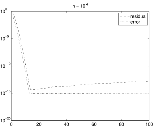
Fig. 3: The residual and true error norms in the Chebyshev algorithm to compute $y_{m}\approx\exp(-A)v$ against iteration number $m$. Normal matrix $A\in\mathbb{R}^{n\times n}$. Top: $n=10^{4}$. Bottom: $n=10^{5}$.

6.1 Residual in Chebyshev iteration

The following tests are carried out for the Chebyshev iterative method with incorporated residual control (see Figure 1). We compute $\exp(-A)v$, where $v\in\mathbb{R}^{n}$ is a random vector with mean zero and standard deviation one. In the first test, the matrix $A\in\mathbb{R}^{n\times n}$ is diagonal with diagonal entries evenly distributed between $-1$ and $1$. In the second test, we fill the first superdiagonal of $A$ with ones, so that $A$ becomes ill-conditioned. The plots of the error and residual norms are presented in Figures 3 and 4.

Fig. 4: The residual and true error norms in the Chebyshev algorithm to compute $y_{m}\approx\exp(-A)v$ against iteration number $m$. Nonnormal matrix $A\in\mathbb{R}^{n\times n}$. Top: $n=10^{4}$. Bottom: $n=10^{5}$.

As can be expected, for nonnormal $A$ the error accumulates during the iteration, so it is important to know when to stop the iteration. Too many iterations may yield a completely wrong answer. The residual sharply reflects the error behavior, thus providing a reliable error estimate.

6.2 A convection-diffusion problem

In the next several numerical experiments the matrix $A$ is taken to be the standard five-point central difference discretization of the following convection-diffusion operator acting on functions defined in the domain $(x,y)\in[0,1]^{2}$:

$$L[u]=-(D_{1}u_{x})_{x}-(D_{2}u_{y})_{y}+\textit{P\!e}{}(v_{1}u_{x}+v_{2}u_{y}),$$

$$D_{1}(x,y)=\begin{cases}10^{3}\;&(x,y)\in[0.25,0.75]^{2},\\ 1&\text{otherwise},\end{cases}\qquad\quad D_{2}(x,y)=\frac{1}{2}D_{1}(x,y),$$

$$v_{1}(x,y)=x+y,\qquad v_{2}(x,y)=x-y.$$

To guarantee that the convection terms yield an exactly skew-symmetric matrix, before discretizing we rewrite the convection terms in the form [24]

$$v_{1}u_{x}+v_{2}u_{y}=\frac{1}{2}(v_{1}u_{x}+v_{2}u_{y})+\frac{1}{2}((v_{1}u)_{x}+(v_{2}u)_{y}).$$

This is possible because the velocity field $(v_{1},v_{2})$ is divergence free. The operator $L$ is set to satisfy the homogeneous Dirichlet boundary conditions. The discretization is done on a $102\times 102$ or $402\times 402$ uniform mesh, producing an $n\times n$ matrix $A$ of size $n=10^{4}$ or $n=16\times 10^{4}$, respectively. The Peclet number varies from $\textit{P\!e}{}=0$ (no convection, $A=A^{T}$) to $\textit{P\!e}{}=10^{3}$, which on the finer mesh means $\|A-A^{T}\|_{1}/\|A+A^{T}\|_{1}\approx 8\times 10^{-4}$.

Table 2: Performance of the exponential Richardson method for the convection-diffusion test problem, $\mathtt{toler}=10^{-4}$, $M=\mathrm{tridiag}(A)$. The CPU times are measured on a 3GHz Linux PC. We emphasize that the CPU time measurements are made in Matlab and thus are only an approximate indication of the actual performance.

	flops/$n$,	matvecs	LU	solving	error
	CPU time, s	$A$ / steps	$I+\alpha M$	$I+\alpha M$
$\textit{P\!e}=0$
EXPOKIT	4590, 2.6	918 matvecs	—	—	1.20e$-$11
exp. Richardson	2192, 1.7	8 steps	24	176	2.21e$-$04
$\textit{P\!e}=10$
EXPOKIT	4590, 2.6	918 matvecs	—	—	1.20e$-$11
exp. Richardson	2202, 1.7	8 steps	29	176	2.25e$-$04
$\textit{P\!e}=100$
EXPOKIT	4590, 2.6	918 matvecs	—	—	1.20e$-$11
exp. Richardson	2492, 1.9	9 steps	31	200	4.00e$-$04

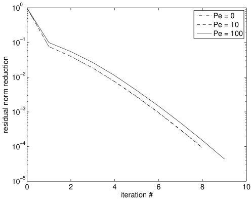
Fig. 5: Convergence history of the exponential Richardson iteration

6.3 Exponential Richardson iteration

In this section we apply the exponential Richardson iteration (32), (33) to compute the vector $\exp(-A)v$ for the convection-diffusion matrices $A$ described in Section 6.2. The mesh is taken to be $102\times 102$. As discussed above, to be able to update the residual and solve the IVP (33), we need to store the values of $r_{k}(t)$ for different $t$ spanning the time interval of interest. Too few samples may result in an accuracy loss in the interpolation stage. On the other hand, it can be prohibitively expensive to store many samples. Therefore, in its current form, the method does not seem practical if a high accuracy is needed. On the other hand, it turns out that with relatively few samples ($\approx 20$) a moderate accuracy up to $10^{-5}$ can be reached.

We organize the computations in the method as follows. The residual vector function $r_{k}(t)$ is stored as 20 samples. At each iteration, the IVP (33) is solved by the Matlab ode15s ODE solver, and the values of the right-hand side function $-M\tilde{\epsilon}_{k}(t)+r_{k}(t)$ are interpolated using the stored samples. The ode15s solver is run with tolerances determined by the final required accuracy and produces the solution $\tilde{\epsilon}_{k}(t)$ in the form of its twenty samples. Then, the solution and residual are updated according to (32) and (35) respectively.

We have chosen $M$ to be the tridiagonal part $\mathrm{tridiag}(A)$ of the matrix $A$. Table 2 and Figure 5 contains results of the test runs. Except the Richardson method, as a reference we use the EXPOKIT code [34] with the maximal Krylov dimension 100. Note that EXPOKIT provides a much accurate solution than requested by the tolerance $\mathtt{toler}=10^{-4}$.

It is rather difficult to compare the total computational work of the EXPOKIT and Richardson methods exactly. We restrict ourselves to the matrix-vector part of the work. In the Richardson method this work consists of the matrix-vector multiplication (matvec) with $M-A$ in (35) and the work done by the ode15s solver. The matvec with bidiagonal $M-A$ costs about $3n$ flops times 20 samples, in total $60n$ flops. The linear algebra work in ode15s is essentially tridiagonal matvecs, LU factorizations and back/forward substitutions with (possibly shifted and scaled) $M$. According to [13, Section 4.3.1], tridiagonal LU factorization, back- and forward substitution require about $2n$ flops each. A matvec with tridiagonal $M$ is $5n$ flops. Thus, in total exponential Richardson costs $60n$ flops times the number of iterations plus $2n$ flops times the number of LU factorizations and back/forward substitutions plus $5n$ flops times the total number of ODE solver steps. The matvec work in EXPOKIT consists of matvecs with pentadiagonal $A$, which is about $9n$ flops.

From Table 2 we see that exponential Richardson is approximately twice as cheap as EXPOKIT. As expected from the convergence estimates, exponential Richardson converges much faster than the conventional Richardson iteration for solving a linear system $Ax=v$ would do. For these $A$ and $v$, 8–9 iterations of the conventional Richardson would only give a residual reduction by a factor of $\approx 0.99$.

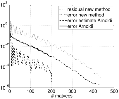
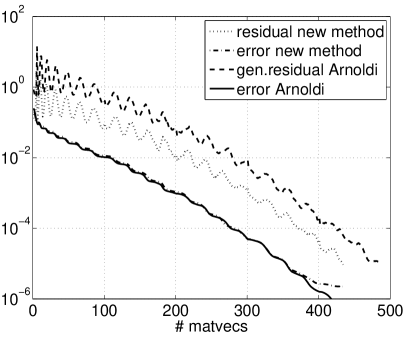
Fig. 6: Convergence of the conventional Arnoldi method with two existing stopping criteria and Krylov-Richardson with the residual-based stopping criterion for tolerance $\mathtt{toler}=10^{-5}$. Left: stagnation-based criterion, Arnoldi stops too early (201 matvecs, 2.6 s CPU time, error 1.0e$-$03). Right: generalized residual criterion, Arnoldi stops too late (487 matvecs, 139 s CPU time, error 4.9e$-$08). Parameters of the Krylov-Richardson run for both plots: 434 matvecs, 11 s CPU time, error 2.2e$-$06). The CPU measurements (on a 3GHz Linux PC) are made in Matlab and thus are only an indication of the actual performance.

6.4 Experiments with Krylov-Richardson iteration

In this section we present some numerical experiments with the Krylov-Richardson method presented in Section 5.2. We now briefly describe the other methods to which Krylov-Richardson is compared.

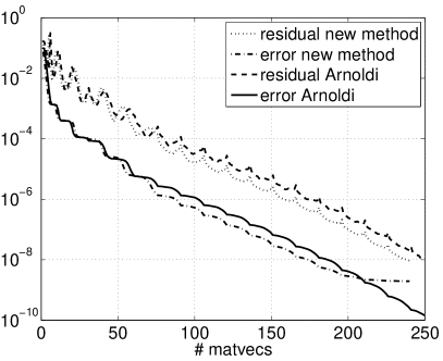
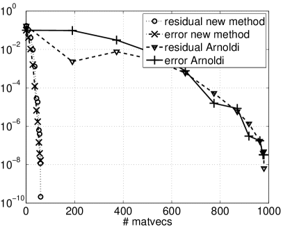
Fig. 7: Convergence plots of the Arnoldi/Lanczos and the new Krylov-Richardson methods, mesh $102\times 102$, $\textit{P\!e}{}=100$. Left: restart every 15 steps, right: SaI strategy with GMRES. The peaks in the residual plots on the left correspond to the restarts.

Together with the classical Arnoldi/Lanczos method [11, 31, 6, 17], we have tested the SaI method of Van den Eshof and Hochbruck [37]. We have implemented the method exactly as described in their paper, with a single modification. In particular, as advised by the authors, in all the tests the shift parameter $\gamma$ is set to $0.1t_{\text{end}}$ and the relaxed stopping criterion strategy for the inner iterative SaI solvers is employed. The only thing we have changed is the stopping criterion of the outer Krylov process. To be able to exactly compare the computational work, we can switch from the stopping criterion of Van den Eshof and Hochbruck (based on iteration stagnation) to the residual stopping criterion (see Lemma 2). Note that the relaxed strategy for the inner SaI solver is then also based on the residual norm and not on the error estimate.

Since the Krylov-Richardson method is essentially a restarting technique, it has to be compared with other existing restarting techniques. Note that a number of restarting strategies have recently been developed [36, 1, 14, 8, 29]. We have used the restarting method described in [29]. This choice is motivated by the fact that the method from [29] turns out to be algorithmically very close to our Krylov-Richardson method. In fact, the only essential difference is handling of the projected problem. In the method [29] the projected matrix $H_{k}$ built up at every restart is appended to a larger matrix $\widetilde{H}_{*+k}$. There, the projected matrices from each restart are accumulated. Thus, if 10 restarts of 20 steps are done, we have to compute the matrix exponential of a $200\times 200$ matrix. In our method, the projected matrices are not accumulated, so at every restart we deal with a $20\times 20$ matrix. The price to pay, however, is the solution of the small IVP (40).

In our implementation, at each Krylov-Richardson iteration the IVP (40) is solved by the ode15s ODE solver from Matlab. To save computational work, it is essential that the solver be called most of the time with a relaxed tolerance (in our code we set the tolerance to 1% of the current residual norm). This is sufficient to estimate the residual accurately. Only when the actual solution update takes place (see formula (37)) do we solve the projected IVP to a full accuracy.

Since the residual time dependence in Krylov-Richardson is given by a scalar function, little storage is needed for the look-up table. Based on the required accuracy, the ode15s solver automatically determines how many samples need to be stored (in our experiments this usually did not exceed 300). This happens at the end of each restart or when the stopping criterion is satisfied. Further savings in computational work can be achieved by a polynomial fitting: at each restart the newly computed values of the function $\psi_{k}$ (see (38)) are approximated by a best-fit polynomial of a moderate degree (in all experiments the degree was set to 6). If the fitting error is too large (this depends on the required tolerance), the algorithm proceeds as before. Otherwise, the $\psi_{k}$ function is replaced by its best-fit polynomial. This allows a faster solution of the projected IVP (40) through an explicit formula containing the functions

$$\varphi_{k}(x)=\frac{\varphi_{k-1}(x)-\varphi_{k-1}(0)}{x},\quad k\geqslant 1,\quad\varphi_{0}=e^{x}.$$

We now present an experiment showing the importance of a proper stopping criterion. We compute $\exp(-5A)v$ for $A$ being the convection-diffusion operator discretized on a uniform mesh $102\times 102$ with $\textit{P\!e}{}=100$. The tolerance is set to $\mathtt{toler}=10^{-5}$. We let the usual Arnoldi method, restarted every 100 steps, run with the stagnation-based stopping criterion of [37] and with the stopping criterion of [18] based on the generalized residual (9). We emphasize that the stagnation-based stopping criterion of [37] is proposed for the Arnoldi method with SaI strategy and it works, in our limited experience, very well as soon as SaI is employed. However, the stagnation-based stopping criteria are used in Krylov methods not only with SaI (see e.g. [3]) and it is instructive to see possible implications of it. Together with Arnoldi, the Krylov-Richardson method is run with the residual-based stopping criterion. The convergence plots are shown in Figure 6. As we see, both existing stopping criteria turn out to be far from optimal in this test. With the residual-based stopping criterion, the Arnoldi method required 438 matvecs and 78 s CPU time to obtain an adequate accuracy of 4.5e$-$7.

Table 3: Results of the test runs of the Krylov-Richardson and Arnoldi with the residual-based stopping criterion. The CPU times are measured on a 2GHz Mac PC (mesh $102\times 102$) and on a 3GHz Linux PC (mesh $402\times 402$). We emphasize that the CPU time measurements are made in Matlab and thus are only an approximate indication of the actual performance.

	restart / SaI	total matvecs	CPU	error
		or LU actions	time
mesh $102\times 102$, $\textit{P\!e}=100$
EXPOKIT	restart 15	1343	2.2	3.61e$-$09
Arnoldi	restart 15	250	26.4	1.45e$-$10
new method	restart 15	240	6.7	1.94e$-$09
EXPOKIT	restart 100	1020	7.6	1.33e$-$11
Arnoldi	restart 100	167	7.9	1.21e$-$10
new method	restart 100	168	11.8	1.14e$-$10
Arnoldi	SaI/GMRESa	980 (11 steps)	17.8	3.29e$-$08
new method	SaI/GMRESa	60 (10 steps)	1.7	1.67e$-$08
Arnoldi	SaI/sparse LU	“11” (10 steps)	1.7	3.62e$-$09
new method	SaI/sparse LU	“11” (10 steps)	1.8	1.61e$-$10
mesh $402\times 402$, $\textit{P\!e}=1000$
EXPOKIT	restart 15	1445	21	4.36e$-$09
Arnoldi	restart 15	244	11	1.13e$-$10
new method	restart 15	254	15	2.62e$-$09
EXPOKIT	restart 100	1020	69	1.33e$-$11
Arnoldi	restart 100	202	34	1.06e$-$10
new method	restart 100	200	35	3.62e$-$10
Arnoldi	SaI/GMRESa	1147 (15 steps)	80	5.68e$-$08
new method	SaI/GMRESa	97 (12 steps)	6.2	1.28e$-$08
Arnoldi	SaI/sparse LU	“12” (11 steps)	46	3.06e$-$08
new method	SaI/sparse LU	“13” (12 steps)	50	2.07e$-$10
a GMRES(100) with SSOR preconditioner

To facilitate a fare comparison between the conventional Arnoldi and the Krylov-Richardson methods, in all the other tests we use the residual-based stopping criterion for both methods. Table 3 and Figures 7 contain the results of the test runs to compute $\exp(-A)v$ for tolerance $\mathtt{toler}=10^{-8}$. We show the results on two meshes for two different Peclet numbers only, the results for other Peclet numbers are quite similar.

The first observation we make is that the CPU times measured in Matlab seem to favor the EXPOKIT code, disregarding the actual matvec values. We emphasize that when the SaI strategy is not used, the main computational cost in all the three methods, EXPOKIT, Arnoldi and Krylov-Richardson, are $k$ steps of the Arnoldi/Lanczos process. The differences among the three methods correspond to the rest of the computational work, which is $\mathcal{O}(k^{3})$, if at least if not too many restarts are made.

The second observation is that the convergence of the Krylov-Richardson iteration is essentially the same as of the classical Arnoldi/Lanczos method. This is not influenced by the restart value or by the SaI strategy. Theoretically, this is to be expected: the former method applies Krylov for the $\varphi$ function, the latter for the exponential; for both functions similar convergence estimates hold, though they are slightly more favorable for the $\varphi$ function [17].

When no SaI strategy is applied, the gain we have with Krylov-Richardson is two-fold. First, a projected problem of much smaller size has to be solved. This is reflected by the difference in the CPU times of Arnoldi and Krylov-Richardson with restart 15 in lines 2 and 3 of the Table: 26.4 s and 6.7 s. Of course, this effect can be less pronounced for larger problems or on faster computers—see the corresponding lines for Arnoldi and Krylov-Richardson with restart 15 on a finer mesh. Second, we have some freedom in choosing the initial vector (in standard Arnoldi/Lanczos we must always start with $v$). This freedom is not complete because the residual of the initial guess has to have scalar dependence on time. Several variants for choosing the initial vector exist, and we will explore these possibilities in the future.

A significant reduction in total computational work can be achieved when Krylov-Richardson is combined with the SaI strategy. The gain is then due to the reduction in the number of the inner iterations (the number of outer iterative steps is approximately the same). In our limited experience, this is not always the case but typically takes place when, for instance, $v$ and $A$ represent discretizations of a smooth function and a smooth partial differential operator, respectively. Currently, we do not completely understand this behavior. Apparently, the Krylov subspace vectors built in the Krylov-Richardson method constitute more favorable right-hand sides for the inner SaI solvers to converge. It is rather difficult to analyze this phenomenon, but we will try to do this in the near future.

6.5 Initial vector and Krylov subspace convergence

It is instructive to observe dependence of the Krylov subspace methods on the initial vector $v$. In particular, if (3) stems from an initial-boundary-value problem (IBVP) and $A$ is a discretized partial differential operator, a faster convergence may take place for $v$ satisfying boundary conditions of the problem. Note that for the convection-diffusion test problem from the previous section this effect is not pronounced ($v$ did not satisfy boundary conditions), probably due to the jump in the diffusion coefficients. We therefore demonstrate this effect on a simple IBVP

$$u_{t}=\Delta u,\qquad u(x,y,z,0)=u_{0}(x,y,z),$$ (44)

posed for $(x,y,z)\in[0,1]^{3}$ for unknown function $u(x,y,z,t)$ obeying periodic boundary conditions. We use a fourth-order finite volume discretization in space from [41] on a regular mesh $40\times 40\times 40$ and arrive at IVP (3) which we solve for $t=1000$ by computing $\exp(-tA)v$. In Figure 8 convergence of the Krylov-Richardson and Arnoldi/Lanczos methods is illustrated for the starting vector $v$ corresponding to

$$u_{0}(x,y,z)=\sin(2\pi x)\sin(2\pi y)\sin(2\pi z)+x(a-x)y(a-y)z(a-z),$$

with $a=2$ or $a=1$. In both cases the restart value is set to 100. The second choice $a=1$ (right plot) agrees with boundary conditions in the sense that $u_{0}$ can be periodically extended and leads to a faster convergence. The same effect is observed for the Krylov-Richardson and Arnoldi/Lanczos methods with the SaI strategy, with a reduction in the number of steps from 12 to 8 or 9. Remarkably, EXPOKIT(100) converges for both choices of $v$ within the same number of steps, 306. Apparently, this is because EXPOKIT splits the given time interval $[0,t_{\text{end}}]$, building for each subinterval a new Krylov subspace.

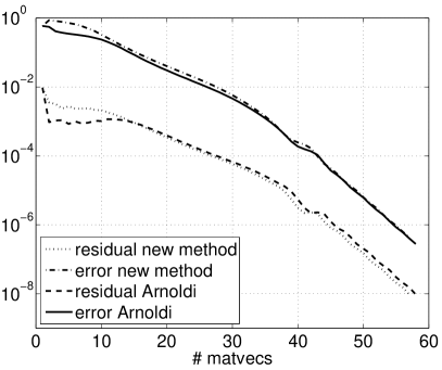
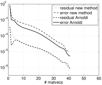
Fig. 8: Convergence plots of the Arnoldi/Lanczos and the new Krylov-Richardson methods for the fourth-order finite volume discretization of the three-dimensional Laplacian with periodic boundary conditions. Left: the starting vector $v$ disobeys the boundary conditions, right: $v$ is consistent with the boundary conditions.

7 Concluding remarks and an outlook to further research

The proposed residual notion appears to provide a reliable stopping criterion in the iterative methods for computing the matrix exponential. This is confirmed by the numerical tests and analysis. Furthermore, the residual concept seems to set up a whole framework for a new class of methods for evaluating the matrix exponential. Some basic methods of this class are proposed in this paper. Many new research questions arise. One of them is a comprehensive convergence analysis of the new exponential Richardson and Krylov-Richardson methods. Another interesting research direction is development of other residual-based iterative methods. In particular, one may ask whether the exponential Richardson method (32)–(33) can not be used as a preconditioner for the Krylov-Richardson method (37). We plan to address this question in future.

Finally, an interesting question is whether the proposed residual notion can be extended to other matrix functions. This is possible once a residual equation can be identified, i.e. an equation such that the matrix function satisfies this equation (see Table 1). For example, if we are interested in computing the vector $u=\cos(A)v$, for given $A\in\mathbb{R}^{n\times n}$ and $v\in\mathbb{R}^{n}$, then we may consider a vector function $u(t)=\cos(tA)v$, which is a solution of the IVP

$$u^{\prime\prime}(t)=-A^{2}u,\quad u(0)=v,\quad u^{\prime}(0)=0.$$

Thus, for an approximate solution $u_{k}(t)\approx u(t)$ satisfying the initial conditions, the residual can be introduced as

$$r_{k}(t)\equiv-A^{2}u_{k}(t)-u_{k}^{\prime\prime}(t).$$

References

- [1] M. Afanasjew, M. Eiermann, O. G. Ernst, and S. Güttel. Implementation of a restarted Krylov subspace method for the evaluation of matrix functions. Linear Algebra Appl., 429:2293–2314, 2008.
- [2] M. Benzi and N. Razouk. Decay bounds and algorithms for approximating functions of sparse matrices. Electron. Trans. Numer. Anal., 28:16–39, 2007.
- [3] M. A. Botchev, D. Harutyunyan, and J. J. W. van der Vegt. The Gautschi time stepping scheme for edge finite element discretizations of the Maxwell equations. J. Comput. Phys., 216:654–686, 2006. http://dx.doi.org/10.1016/j.jcp.2006.01.014.
- [4] V. Druskin, A. Greenbaum, and L. Knizhnerman. Using nonorthogonal Lanczos vectors in the computation of matrix functions. SIAM J. Sci. Comput., 19(1):38–54, 1998. Special issue on iterative methods (Copper Mountain, CO, 1996).
- [5] V. L. Druskin and L. A. Knizhnerman. Two polynomial methods of calculating functions of symmetric matrices. U.S.S.R. Comput. Maths. Math. Phys., 29(6):112–121, 1989.
- [6] V. L. Druskin and L. A. Knizhnerman. Krylov subspace approximations of eigenpairs and matrix functions in exact and computer arithmetic. Numer. Lin. Alg. Appl., 2:205–217, 1995.
- [7] V. L. Druskin and L. A. Knizhnerman. Extended Krylov subspaces: approximation of the matrix square root and related functions. SIAM J. Matrix Anal. Appl., 19(3):755–771 (electronic), 1998.
- [8] M. Eiermann, O. G. Ernst, and S. Güttel. Deflated restarting for matrix functions. Submitted, October 2009.
- [9] W. H. Enright. Continuous numerical methods for ODEs with defect control. J. Comput. Appl. Math., 125(1-2):159–170, 2000. Numerical analysis 2000, Vol. VI, Ordinary differential equations and integral equations.
- [10] A. Frommer and V. Simoncini. Matrix functions. In W. H. A. Schilders, H. A. van der Vorst, and J. Rommes, editors, Model Order Reduction: Theory, Research Aspects and Applications, pages 275–304. Springer, 2008.
- [11] E. Gallopoulos and Y. Saad. Efficient solution of parabolic equations by Krylov approximation methods. SIAM J. Sci. Statist. Comput., 13(5):1236–1264, 1992.
- [12] F. R. Gantmacher. The Theory of Matrices. Vol. 1. AMS Chelsea Publishing, Providence, RI, 1998. Translated from the Russian by K. A. Hirsch, Reprint of the 1959 translation.
- [13] G. H. Golub and C. F. Van Loan. Matrix Computations. The Johns Hopkins University Press, Baltimore and London, third edition, 1996.
- [14] S. Güttel. Rational Krylov Methods for Operator Functions. PhD thesis, Technischen Universität Bergakademie Freiberg, March 2010. www.guettel.com.
- [15] N. J. Higham. Functions of Matrices: Theory and Computation. Society for Industrial and Applied Mathematics, Philadelphia, PA, USA, 2008.
- [16] N. J. Higham and A. H. Al-Mohy. Computing matrix functions. Acta Numer., 19:159–208, 2010.
- [17] M. Hochbruck and C. Lubich. On Krylov subspace approximations to the matrix exponential operator. SIAM J. Numer. Anal., 34(5):1911–1925, Oct. 1997.
- [18] M. Hochbruck, C. Lubich, and H. Selhofer. Exponential integrators for large systems of differential equations. SIAM J. Sci. Comput., 19(5):1552–1574, 1998.
- [19] M. Hochbruck and A. Ostermann. Exponential integrators. Acta Numer., 19:209–286, 2010.
- [20] J. Janssen and S. Vandewalle. On SOR waveform relaxation methods. SIAM J. Numer. Anal., 34(6):2456–2481, 1997.
- [21] J. Kierzenka and L. F. Shampine. A BVP solver that controls residual and error. JNAIAM J. Numer. Anal. Ind. Appl. Math., 3(1-2):27–41, 2008.
- [22] L. Knizhnerman and V. Simoncini. A new investigation of the extended Krylov subspace method for matrix function evaluations. Numer. Linear Algebra Appl., 2009. To appear.
- [23] L. A. Knizhnerman. Calculation of functions of unsymmetric matrices using Arnoldi’s method. U.S.S.R. Comput. Maths. Math. Phys., 31(1):1–9, 1991.
- [24] L. A. Krukier. Implicit difference schemes and an iterative method for solving them for a certain class of systems of quasi-linear equations. Sov. Math., 23(7):43–55, 1979. Translation from Izv. Vyssh. Uchebn. Zaved., Mat. 1979, No. 7(206), 41–52 (1979).
- [25] C. Lubich. From quantum to classical molecular dynamics: reduced models and numerical analysis. Zurich Lectures in Advanced Mathematics. European Mathematical Society (EMS), Zürich, 2008.
- [26] A. Lumsdaine and D. Wu. Spectra and pseudospectra of waveform relaxation operators. SIAM J. Sci. Comput., 18(1):286–304, 1997. Dedicated to C. William Gear on the occasion of his 60th birthday.
- [27] C. B. Moler and C. F. Van Loan. Nineteen dubious ways to compute the exponential of a matrix, twenty-five years later. SIAM Rev., 45(1):3–49, 2003.
- [28] I. Moret and P. Novati. RD rational approximations of the matrix exponential. BIT, 44:595–615, 2004.
- [29] J. Niehoff. Projektionsverfahren zur Approximation von Matrixfunktionen mit Anwendungen auf die Implementierung exponentieller Integratoren. PhD thesis, Mathematisch-Naturwissenschaftlichen Fakultät der Heinrich-Heine-Universität Düsseldorf, December 2006.
- [30] V. S. Ryaben′kii and S. V. Tsynkov. A Theoretical Introduction to Numerical Analysis. Chapman & Hall/CRC, Boca Raton, FL, 2007.
- [31] Y. Saad. Analysis of some Krylov subspace approximations to the matrix exponential operator. SIAM J. Numer. Anal., 29(1):209–228, 1992.
- [32] Y. Saad. Iterative Methods for Sparse Linear Systems. Book out of print, 2000. www-users.cs.umn.edu/~saad/books.html.
- [33] L. F. Shampine. Solving ODEs and DDEs with residual control. Appl. Numer. Math., 52(1):113–127, 2005.
- [34] R. B. Sidje. Expokit. A software package for computing matrix exponentials. ACM Trans. Math. Softw., 24(1):130–156, 1998. www.maths.uq.edu.au/expokit/.
- [35] H. Tal-Ezer. Spectral methods in time for parabolic problems. SIAM J. Numer. Anal., 26(1):1–11, 1989.
- [36] H. Tal-Ezer. On restart and error estimation for Krylov approximation of . SIAM J. Sci. Comput., 29(6):2426–2441 (electronic), 2007.
- [37] J. van den Eshof and M. Hochbruck. Preconditioning Lanczos approximations to the matrix exponential. SIAM J. Sci. Comput., 27(4):1438–1457, 2006.
- [38] H. A. van der Vorst. An iterative solution method for solving , using Krylov subspace information obtained for the symmetric positive definite matrix . J. Comput. Appl. Math., 18:249–263, 1987.
- [39] H. A. van der Vorst. Iterative Krylov methods for large linear systems. Cambridge University Press, 2003.
- [40] J. L. M. van Dorsselaer, J. F. B. M. Kraaijevanger, and M. N. Spijker. Linear stability analysis in the numerical solution of initial value problems. In Acta numerica, 1993, pages 199–237. Cambridge Univ. Press, Cambridge, 1993.
- [41] R. W. C. P. Verstappen and A. E. P. Veldman. Symmetry-preserving discretization of turbulent flow. J. Comput. Phys., 187(1):343–368, 2003. http://dx.doi.org/10.1016/S0021-9991(03)00126-8.
- [42] V. A. Zorich. Mathematical analysis I. Springer-Verlag, Berlin, 2009. Translated from Russian.