Riemann Solver for a Kinematic Wave Traffic Model with Discontinuous Flux

Abstract

We investigate a model for traffic flow based on the Lighthill–Whitham–Richards model that consists of a hyperbolic conservation law with a discontinuous, piecewise-linear flux. A mollifier is used to smooth out the discontinuity in the flux function over a small distance $\epsilon\ll 1$ and then the analytical solution to the corresponding Riemann problem is derived in the limit as $\epsilon\rightarrow 0$. For certain initial data, the Riemann problem can give rise to zero waves that propagate with infinite speed but have zero strength. We propose a Godunov-type numerical scheme that avoids the otherwise severely restrictive CFL constraint that would arise from waves with infinite speed by exchanging information between local Riemann problems and thereby incorporating the effects of zero waves directly into the Riemann solver. Numerical simulations are provided to illustrate the behaviour of zero waves and their impact on the solution. The effectiveness of our approach is demonstrated through a careful convergence study and comparisons to computations using a third-order WENO scheme.

url]http://www.math.sfu.ca/ stockie

1 Introduction

In the 1950’s, Lighthill and Whitham [30] and Richards [36] independently proposed the first macroscopic traffic flow model, now commonly known as the LWR model. Although this model has proven successful in capturing some aspects of traffic behaviour, its limitations are well-documented and many more sophisticated models have been proposed to capture the complex dynamics and patterns observed in actual vehicular traffic [22]. Despite this progress, the LWR model remains an important and widely-used model because of its combination of simplicity and explanatory power.

The LWR model consists of a single scalar nonlinear conservation law in one dimension

$$\rho_{t}+f(\rho)_{x}=0,$$ (1)

where $\rho(x,t)$ is the traffic density (cars/m),

$$f(\rho)=\rho\,v(\rho)$$

is the traffic flow rate or flux (cars/sec), and $v(\rho)$ is the local velocity (m/sec). The most commonly used flux function is

$$f(\rho)=u_{\text{\emph{max}}}\,\rho\left(1-\frac{\rho}{\rho_{\text{\emph{max}}}}\right)\mbox{,}$$ (2)

which was obtained by Greenshields [20] in the 1930’s by fitting experimental measurements of vehicle velocity and traffic density. Here, $u_{max}$ is the maximum free-flow speed, while $\rho_{\text{\emph{max}}}$ is the maximum density corresponding to bumper-to-bumper traffic where speed drops to zero. The LWR model belongs to a more general class of kinematic wave traffic models that couple the conservation law Eq. (1) with a variety of different flux functions.

Extensive studies of the empirical correlation between flow rate and density have been performed in the traffic flow literature. This correlation is commonly referred to as the fundamental diagram and is represented graphically by a plot of flux $f$ versus density $\rho$ such as that shown in Fig. 1. A striking feature of many experimental results is the presence of an apparent discontinuity that separates the free flow (low density) and congested (high density) states, something that has been discussed by many authors, including [7, 14, 15, 23]. In particular, Koshi et al. [24] characterize flux data such as that shown in Fig. 1 as having a reverse lambda shape in which the discontinuity appears at some peak value of the flux.

This behavior is also referred to as the two-capacity or dual-mode phenomenon [3, 4] and has led to the development of a diverse range of mathematical models. Zhang and Kim [41] incorporated the capacity drop into a microscopic car-following model that generates fundamental diagrams with the characteristic reverse-lambda shape. Wong and Wong [38] performed simulations using a multi-class LWR model from which they also observed a discontinuous flux-density relationship. Colombo [8] and Goatin [17] developed a macroscopic model that couples an LWR equation for density in the free flow state, along with a 2$\times$2 system of conservation laws for density and momentum in the congested state; the phase transition between these two states is a free boundary that is governed by the Rankine-Hugoniot conditions. Lu et al. [31] incorporated a discontinuous (piecewise quadratic) flux directly into an LWR model, and then solved the corresponding Riemann problem analytically by constructing the convex hull for a regularized continuous flux function that consists of two quadratic pieces joined over a narrow region by a linear connecting piece.

There remains some disagreement in the literature regarding the existence of discontinuities in the traffic flux, with some researchers (e.g., Hall [21]) arguing that the apparent gaps are due simply to missing data and can be accounted for by providing additional information about traffic behaviour at specific locations. Indeed, Persaud and Hall [35] and Wu [39] contend that the discontinuous fundamental diagram should be viewed instead as the 2D projection of a higher dimensional smooth surface.

We will nonetheless make the assumption in this paper that the fundamental diagram is discontinuous. Our aim here is not to argue the validity of this assumption in the context of traffic flow, since that point has already been discussed extensively by [31, 38, 41], among others. Instead our objective is to study the effect that such a flux discontinuity has on the analytical solution of a 1D hyperbolic conservation law, as well as to develop an accurate and efficient numerical algorithm to simulate such problems.

A related class of conservation laws, in which the flux $f(\rho,x)$ is a discontinuous function of the spatial variable $x$, has been thoroughly studied in recent years (see [5, 6] and the references therein). Considerably less attention has been paid to the situation where the flux function has a discontinuity in $\rho$. Gimse [16] solved the Riemann problem for a piecewise linear flux function with a single jump discontinuity in $\rho$ by generalizing the method of convex hull construction [28, Ch. 16]. In particular, Gimse identified the existence of zero shocks, which are discontinuities in the solution that carry no information and have infinite speed of propagation. We note that more recently, Armbruster et al. [1] observed zero rarefaction waves with infinite speed of propagation in their study of supply chains with finite buffers (although they did not refer to them using this terminology).

Gimse’s results were improved on by Dias and Figueira [11], who used a mollifier function $\eta_{\epsilon}$ to smooth out discontinuities in the flux function over an interval of width $0<\epsilon\ll 1$ before constructing the convex hull using standard techniques. Solutions to the mollified problem were proven to converge to solutions of the original problem in the limit as $\epsilon\rightarrow 0$ [11]. Dias and Figueira’s framework has also been applied to problems involving fluid phase transitions [10, 13] and viscoelasticity [12].

In this paper, we apply Dias and Figueira’s mollification approach to solving a conservation law with a piecewise linear flux function $f(\rho)$ in which there is a single discontinuity at $\rho=\rho_{m}$ (see Fig. 1). The model equations and their relevance in the context of traffic flow are discussed in Section 2. We introduce a mollified flux function $f_{\epsilon}(\rho)$ in Section 3 and verify its convexity, which then permits us to derive the analytical solution to the Riemann problem using the method of convex hull construction.

In Section 4, we consider the special case where either of the two constant initial states in the Riemann problem equals $\rho_{m}$, the density at the discontinuity point. This is precisely the case when a rarefaction wave of strength $O(\epsilon)$ and speed $O(1/\epsilon)$ arises, which approaches a zero rarefaction in the limit of vanishing $\epsilon$. There are two issues that need to be addressed regarding these zero waves. First, we consider the convergence of the mollified solution to that of the original problem, since Dias and Figueira’s convergence results [11] do not consider (nor easily extend to) the case when the left or right initial states in the Riemann problem are identical to $\rho_{m}$. Secondly, we discuss the physical relevance of an infinite speed of propagation in the context of traffic flow.

The remainder of the paper is focused on constructing a Riemann solver that forms the basis for a high resolution finite volume scheme of Godunov type. Because zero waves travel at infinite speed, the usual CFL restriction suggests that choosing a stable time step might not be possible. Some authors have avoided this difficulty by using an implicit time discretization [33], but this approach introduces added expense and complication in the numerical algorithm. Another approach employed in [1] is to replace the discontinuous flux by a regularized (continuous) function which joins the discontinuous pieces by a linear connection over an interval of width $\epsilon\ll 1$, after which standard numerical schemes may be applied; however, this approach requires a small $\epsilon$ to achieve reasonable accuracy resulting in a severe time step restriction.

We use an alternate approach that eliminates the severe CFL constraint by incorporating the effect of zero waves directly into the local Riemann solver. In the process, we find it necessary to construct solutions to a subsidiary problem that we refer to as the double Riemann problem, which introduces an additional intermediate state corresponding to the discontinuity value $\rho=\rho_{m}$. A similar approach was used by Gimse [16] who constructed a first-order variant of Godunov’s method, although he omitted to perform any computations using his proposed method. We improve upon Gimse’s work in three ways: first, we solve the double Riemann problem within Dias and Figueira’s mollification framework; second, we implement a high resolution variant of Godunov’s scheme to increase the spatial accuracy; and third, we provide extensive numerical computations and a careful convergence study to demonstrate the effectiveness of our approach.

2 Mathematical Model

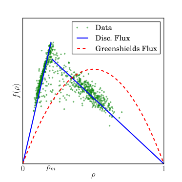
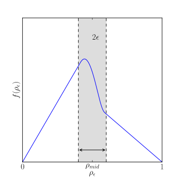
Figure 1: In 1, the discontinuous “reverse lambda” flux function Eq. (4) is overlaid with empirical data extracted from [21, Fig. 7] (reproduced with permission of Elsevier B.V.), along with the quadratic Greenshields flux (2). The mollified flux from Eq. (7) is depicted in 1.

We are concerned in this paper with the scalar conservation law

$$\rho_{t}+f(\rho)_{x}=0,$$ (3)

having a discontinuous flux function

$$f(\rho)=\left\{\begin{array}[]{ll}\displaystyle g_{\mathit{f}}(\rho),&\text{if}~{}0\leqslant\rho<\rho_{m},\\ \displaystyle g_{\mathit{c}}(\rho),&\text{if}~{}\rho_{m}\leqslant\rho\leqslant 1,\end{array}\right.$$ (4)

that is depicted in Fig. 11. The vehicle density $\rho(x,t)$ is normalized so that $0\leqslant\rho\leqslant 1$, and $\rho_{m}$ is the point of discontinuity in the flux $f(\rho)$. We restrict the flux to be a piecewise linear function in which the free flow branch has

$$g_{\mathit{f}}(\rho)=\rho,$$

and the congested flow branch has

$$g_{\mathit{c}}(\rho)=\gamma(1-\rho).$$

Experimental data suggests that $g_{\mathit{f}}(\rho_{m})>g_{\mathit{c}}(\rho_{m})$, and so we impose the constraint

$$0<\gamma<\frac{\rho_{m}}{1-\rho_{m}}\mbox{.}$$ (5)

We utilize the mollifier approach of Dias and Figueira [11] in order to approximate the original equation (3) by

$$\frac{\partial\rho_{\epsilon}}{\partial t}+\frac{\partial f_{\epsilon}(\rho_{\epsilon})}{\partial x}=0,$$ (6)

where the mollified flux (pictured in Fig. 11) is

$$f_{\epsilon}(\rho_{\epsilon})=\rho_{\epsilon}+(\gamma-(\gamma+1)\rho_{\epsilon})\int_{\rho_{m}-\epsilon}^{\rho_{\epsilon}}\eta_{\epsilon}(s-\rho_{m})\,ds\mbox{,}$$ (7)

with $0<\epsilon\ll 1$. The mollifier function is given by $\eta_{\epsilon}(s)=\frac{1}{\epsilon}\eta(s/\epsilon)$, where $\eta(s)$ is a canonical mollifier that satisfies the following conditions:

1. $\eta\geqslant 0$;

2. $\eta\in C^{\infty}(\mathbb{R})$ and is compactly supported on $[-1,1]$;

3. $\eta(-s)=\eta(s)$ for all $s\in\mathbb{R}$; and

4. $\int_{-\infty}^{\infty}\eta(s)\,ds=1$.

The results in Dias and Figueira [11] guarantee that any mollifier satisfying the above criteria converges to the same unique solution in the limit $\epsilon\rightarrow 0$. We use the following mollifier

$$\eta(s)=\left\{\begin{array}[]{ll}C\exp\left(\frac{1}{s^{2}-1}\right),&\text{if}~{}|s|<1,\\ 0,&\text{if}~{}|s|\geqslant 1,\end{array}\right.$$ (8)

where $C\approx 2.2522836\dots$ is a constant determined numerically so that condition (iv) holds; this choice is made for reasons of analytical convenience since the derivative $\eta^{\prime}$ can be written in terms of $\eta$.

Because the mollified flux function is smooth, the conservation law (6) may now be solved using standard techniques. We note that in the context of traffic flow, a potential problem arises when applying the usual Oleĭnik entropy condition [34] as the selection principle to enforce uniqueness. Although Oleĭnik’s entropy condition does yield the physically-correct weak solution in the context of fluid flow applications, it does not always do so for kinematic wave models of traffic flow (see LeVeque [27], for example). In particular, applying Oleĭnik’s entropy condition can lead to a solution that is not anisotropic [9], corresponding to the non-physical situation where drivers react to vehicles both in front and behind.

Zhang [40] suggests two additional criteria on the flux function to guarantee anisotropic flows in kinematic wave traffic models. First, the characteristic velocity should be smaller than the vehicle speed $v(\rho)=f(\rho)/\rho$. That is, we require

$$\frac{f(\rho)}{\rho}\geq f^{\prime}(\rho),~{}~{}\forall~{}0\leq\rho\leq 1.$$

Secondly, all elementary waves must travel more slowly than the vehicles carrying them, or

$$\min\left(\frac{f(\rho_{l})}{\rho_{l}},~{}\frac{f(\rho_{r})}{\rho_{r}}\right)\geq\frac{f(\rho_{r})-f(\rho_{l})}{\rho_{r}-\rho_{l}},$$

for all $0\leq\rho_{l},\rho_{r}\leq 1$. As shown in [37], our flux function (4) satisfies both of these conditions and therefore it is reasonable to apply the Oleĭnik entropy condition as the selection criterion for our traffic flow model.

3 Exact Solution of the Riemann Problem with Mollified Flux

We next construct and analyze the solution $\rho_{\epsilon}(x,t)$ of the mollified Riemann problem, which consists of the conservation law (6) along with flux (7) and piecewise constant initial conditions

$$\rho_{\epsilon}(x,0)=\left\{\begin{array}[]{ll}\rho_{l},&\text{if}~{}x<0,\\ \rho_{r},&\text{if}~{}x\geqslant 0.\end{array}\right.$$

This problem can be solved using the method of convex hull construction [28, Ch. 16] which requires knowledge of the inflection points of the mollified flux $f_{\epsilon}(\rho_{\epsilon})$. Using Eq. (8), the first and second derivatives of the flux are

$$f_{\epsilon}^{\prime}(\rho_{\epsilon}) =1+\left[\gamma-(\gamma+1)\rho_{\epsilon}\right]\,\eta_{\epsilon}(\rho_{\epsilon}-\rho_{m})-(\gamma+1)\int_{\rho_{m}-\epsilon}^{\rho_{\epsilon}}\eta_{\epsilon}(s-\rho_{m})\,ds,$$ (9)

$$f_{\epsilon}^{\prime\prime}(\rho_{\epsilon}) =\kappa(\rho_{\epsilon})\left[\left(\frac{\gamma}{\gamma+1}-\rho_{\epsilon}\right)(\rho_{m}-\rho_{\epsilon})-\epsilon^{2}\left[\left(\frac{\rho_{\epsilon}-\rho_{m}}{\epsilon}\right)^{2}-1\right]^{2}\right],$$ (10)

where

$$\kappa(\rho_{\epsilon})=\frac{2\eta_{\epsilon}(\rho_{\epsilon}-\rho_{m})}{\epsilon^{2}(\gamma+1)[(\frac{\rho_{\epsilon}-\rho_{m}}{\epsilon})^{2}-1]^{2}}.$$

Since the mollifier has compact support, we know that there can be no inflection points outside the smoothing region of width $2\epsilon$; that is, $f_{\epsilon}^{\prime\prime}(\rho_{\epsilon})\equiv 0$ when $|\rho_{\epsilon}-\rho_{m}|\geqslant\epsilon$. Also, since $\kappa(\rho_{\epsilon})>0$, the convexity of $f_{\epsilon}$ is determined solely by the sign of the quantity

$${P}(\rho_{\epsilon})=\left(\frac{\gamma}{\gamma+1}-\rho_{\epsilon}\right)(\rho_{m}-\rho_{\epsilon})-\epsilon^{2}\left[\left(\frac{\rho_{\epsilon}-\rho_{m}}{\epsilon}\right)^{2}-1\right]^{2},$$ (11)

which we analyze next.

Since Eq. (11) is a quartic polynomial in $\rho_{\epsilon}$, analytic expressions are available for the roots; however, these are too complicated for our purposes. Instead, we take advantage of the scaling properties of the polynomial to simplify $P$ and rewrite Eq. (11) as

$$P(y)=-\frac{1}{\epsilon^{2}}y^{4}+3y^{2}+My-\epsilon^{2},$$ (12)

where $y=\rho_{\epsilon}-\rho_{m}\in[-\epsilon,\epsilon]$ and $M=\rho_{m}-\gamma/(\gamma+1)$. Clearly $|y|=|\rho_{\epsilon}-\rho_{m}|<\epsilon$, and so it is natural to suppose that $y=O(\epsilon^{\lambda})$ with $\lambda\geq 1$, after which the various terms in Eq. (12) have the scalings indicated below:

$$P(y)=\underbrace{-\frac{1}{\epsilon^{2}}y^{4}\vphantom{-\frac{1}{\epsilon^{2}}y^{4}}}_{O(\epsilon^{4\lambda-2})}+\underbrace{3y^{2}\vphantom{-\frac{1}{\epsilon^{2}}y^{4}}}_{O(\epsilon^{2\lambda})}+\underbrace{My\vphantom{-\frac{1}{\epsilon^{2}}y^{4}}}_{O(\epsilon^{\lambda})}-\underbrace{\epsilon^{2}\vphantom{-\frac{1}{\epsilon^{2}}y^{4}}}_{O(\epsilon^{2})}\mbox{.}$$ (13)

Since $M$ is a constant that is independent of $\epsilon$, we can take $M=O(1)$ as $\epsilon\rightarrow 0$. Guided by the scalings in Eq. (13), the dominant terms in $P(y)$ are the last two terms having orders $O(\epsilon^{\lambda})$ and $O(\epsilon^{2})$. When $\epsilon$ is sufficiently small, we may therefore neglect the remaining terms and determine the convexity of $f_{\epsilon}$ based on the sign of the simpler linear polynomial

$$P_{1}(y)=My-\epsilon^{2}\mbox{,}$$

which has a single root at $y=\epsilon^{2}/M$ corresponding to $\rho_{\epsilon}=\rho_{m}+\epsilon^{2}/M$. For values of $y$ close enough to $\epsilon^{2}/M$, higher order terms in the polynomial $P(y)$ become significant and could potentially introduce additional roots; however, by continuing this method of dominant balance, we find that $P(y)$ maintains the single root at higher orders as well, which we demonstrate numerically using the plots of $P$ summarized in Fig. 2. Based on this argument and the observation that inequality (5) requires $M>0$, we can conclude that

$$f_{\epsilon}^{\prime\prime}(\rho_{\epsilon})\geqslant 0\quad\mbox{when}\quad\rho_{\epsilon}\in[\rho_{m},1]\mbox{,}$$

and $$f_{\epsilon}^{\prime\prime}(\rho_{\epsilon})\leqslant 0\quad\mbox{when}\quad\rho_{\epsilon}\in[0,\rho_{m}]\mbox{.}$$

Therefore, the mollified flux function has a single inflection point at $\rho_{\epsilon}=\rho_{m}+O(\epsilon^{2})$ as $\epsilon\rightarrow 0$, where the slope $f_{\epsilon}^{\prime}(\rho_{m})\rightarrow-\infty$. Since the flux derivative $f^{\prime}(\rho)$ corresponds to the elementary wave speed in the Riemann problem, this same point $\rho_{m}$ is also the source of the infinite speed of propagation which will be analyzed in more detail in Section 4.

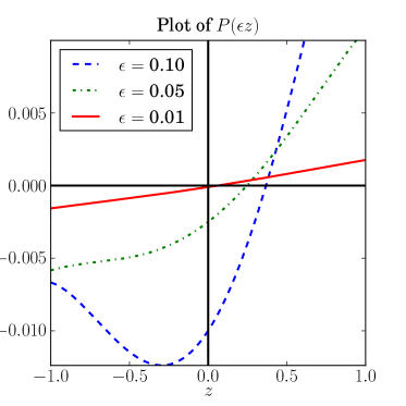
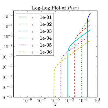
Figure 2: Plots of the function $P(\epsilon z)$ and its roots for different $\epsilon$ when $\gamma=0.5$ and $\rho_{m}=0.5$.

Using this information, we can now construct the convex hull of the flux function $f_{\epsilon}(\rho_{\epsilon})$ which is then used to solve the Riemann problem. There are three non-trivial cases to consider, depending on the left and right initial states, $\rho_{l}$ and $\rho_{r}$. Two of these cases (which we call A and B) lead to the emergence of a new constant intermediate state with density $\rho_{m}$. This “plateau” is a characteristic feature of solutions to our LWR model with discontinuous flux.

Case A: $\boldsymbol{\rho_{r}<\rho_{m}<\rho_{l}}$.

Here we construct the smallest convex hull of the set $\{(\rho_{\epsilon},y):\rho_{r}<\rho_{\epsilon}<\rho_{l}\mbox{ and }y\leqslant f_{\epsilon}(\rho_{\epsilon})\}$, which as shown in Fig. 33 must consist of three pieces. The first piece corresponds to a contact line that follows $f_{\epsilon}(\rho_{\epsilon})$ on the left up to the point $\rho_{*}\in(\rho_{m}-\epsilon,\rho_{m})$ for which the shock and characteristic speeds are equal; that is,

$$s=\frac{f_{\epsilon}(\rho_{l})-f_{\epsilon}(\rho_{*})}{\rho_{l}-\rho_{*}}=f^{\prime}_{\epsilon}(\rho_{*})\mbox{.}$$

The third piece of the convex hull corresponds to a shock that connects the states $\rho_{*}$ and $\rho_{l}$. The middle piece, in between the contact line and shock, gives rise to a rarefaction wave that follows the curved portion of the flux in the neighbourhood of $\rho_{m}$. Based on this convex hull, we can then construct the solution profile shown in Fig. 33. Since the rarefaction wave consists of density values bounded between $\rho_{m}-\epsilon$ and $\rho_{m}+\epsilon$, this wave flattens out and degenerates to a constant intermediate state $\rho_{m}$ in the limit as $\epsilon\rightarrow 0$.

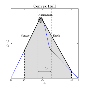
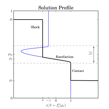
Figure 3: The convex hull construction for Case A. 3 The thin (blue) line is the mollified flux function $f_{\epsilon}(\rho_{\epsilon})$ and the thick (black) line is the convex hull. The shaded oval region highlights the rarefaction wave. 3 The solution $\rho_{\epsilon}(x/t)$ is shown as a thick (black) line, along with the corresponding flux derivative $f^{\prime}(\rho)$ as a thin (blue) line. Parameter values are $\rho_{l}=0.9$, $\rho_{r}=0.2$, $\rho_{m}=0.5$, $\epsilon=0.1$ and $\gamma=0.5$.

To summarize, in the limit as $\epsilon\rightarrow 0$ the solution to the Riemann problem when $\rho_{r}<\rho_{m}<\rho_{l}$ is

$$\rho(x,t)=\left\{\begin{array}[]{ll}\rho_{l},&\text{if}~{}x<st,\\ \rho_{m},&\text{if}~{}st\leqslant x\leqslant t,\\ \rho_{r},&\text{if}~{}x>t,\end{array}\right.$$ (14)

consisting of a 1-shock moving to the left with speed

$$s=\frac{f(\rho_{l})-g_{f}(\rho_{m})}{\rho_{l}-\rho_{m}}<0,$$ (15)

and a 2-contact moving to the right with speed 1.

Case B: $\boldsymbol{\gamma/(\gamma+1)<\rho_{l}<\rho_{m}<\rho_{r}}$.

In contrast with the previous case, we now have $\rho_{l}<\rho_{r}$ and so the convex hull $\{(\rho_{\epsilon},y):\rho_{l}<\rho_{\epsilon}<\rho_{r}\mbox{ and }y\geqslant f_{\epsilon}(\rho_{\epsilon})\}$ lies above the flux-density curve as shown in Fig. 44. The first piece of the convex hull corresponds to a shock wave connecting the states $\rho_{l}$ and $\rho_{*}\in(\rho_{m}-\epsilon,\rho_{m})$, while the third piece follows the portion of the flux function in the region $[\rho_{*},\rho_{r}]$. As before, the state $\rho_{*}$ is chosen so that the shock and characteristic speeds are equal:

$$s=\frac{f_{\epsilon}(\rho_{*})-f_{\epsilon}(\rho_{l})}{\rho_{*}-\rho_{l}}=f^{\prime}_{\epsilon}(\rho_{*})\mbox{.}$$

The resulting solution profile in the limit as $\epsilon\rightarrow 0$ is pictured in Fig. 44:

$$\rho(x,t)=\left\{\begin{array}[]{ll}\rho_{l},&\text{if}~{}x<st,\\ \rho_{m},&\text{if}~{}st\leqslant x\leqslant-\gamma t,\\ \rho_{r},&\text{if}~{}x>-\gamma t,\end{array}\right.$$ (16)

which consists of a 1-shock moving to the left with speed

$$s=\frac{g_{c}(\rho_{m})-f(\rho_{l})}{\rho_{m}-\rho_{l}}<0,$$ (17)

and a 2-contact moving to the left with speed $-\gamma$.

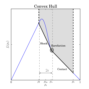
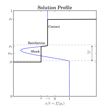
Figure 4: The convex hull construction for Case B. 4 The thin (blue) line is the mollified flux function $f_{\epsilon}(\rho_{\epsilon})$ and the thick (black) line is the convex hull. The shaded oval region highlights the rarefaction wave. 4 The solution $\rho_{\epsilon}(x/t)$ is shown as a thick (black) line, along with the corresponding flux derivative $f^{\prime}(\rho)$ as a thin (blue) line. Parameter values are $\rho_{l}=0.4$, $\rho_{r}=0.9$, $\epsilon=0.1$, $\gamma=0.5$, $\rho_{m}=0.5$.

Case C: $\boldsymbol{\rho_{l}<\rho_{m}<\rho_{r}\;\;\mbox{and}\;\;\gamma/(\gamma+1)\geqslant\rho_{l}}$.

The solution structure in this case is significantly simpler than the previous two in that there is only a single shock connecting the states $\rho_{r}$ and $\rho_{l}$, and hence no intermediate state. The convex hull is depicted in Fig. 55 and the corresponding solution profile in Fig. 55. As $\epsilon\rightarrow 0$, the solution reduces to

$$\rho_{\epsilon}(x,t)=\left\{\begin{array}[]{ll}\rho_{l},&\text{if}~{}x<st,\\ \rho_{r},&\text{if}~{}x\geqslant st,\end{array}\right.$$ (18)

which corresponds to a shock with speed

$$s=\frac{f(\rho_{r})-f(\rho_{l})}{\rho_{r}-\rho_{l}},$$ (19)

which can be either positive or negative depending on the sign of the numerator.

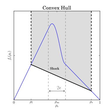
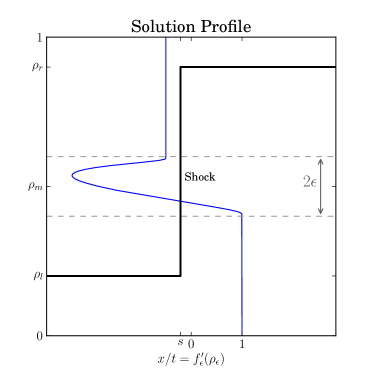
Figure 5: The convex hull construction for Case C. 5 The thin (blue) line is the mollified flux function $f_{\epsilon}(\rho_{\epsilon})$ and the thick (black) line is the convex hull. The shaded oval region highlights the rarefaction wave. 5 The solution $\rho_{\epsilon}(x/t)$ is shown as a thick (black) line, along with the corresponding flux derivative $f^{\prime}(\rho)$ as a thin (blue) line. Parameter values are $\rho_{l}=0.2$, $\rho_{r}=0.9$, $\rho_{m}=0.5$, $\epsilon=0.1$ and $\gamma=0.5$.

Note that as $\rho_{l}$ or $\rho_{r}$ approaches the discontinuity $\rho_{m}$, the Riemann solution becomes sensitive to the choice of initial data. This sensitivity is not unique to our problem, but is also observed in other analytical solutions for problems with discontinuous flux, such as in [13, 16, 31]. In the context of traffic flow, this sensitivity occurs in the neighbourhood of the transition point between free-flow and congested traffic, the exact location of which is expected to be highly sensitive to the state of individual drivers comprising the flow. Therefore, the sensitivity in our model is consistent with actual traffic.

4 Analysis of Zero Waves

In this section, we consider the two special situations that were not addressed in Section 3, namely where either $\rho_{l}=\rho_{m}$ or $\rho_{r}=\rho_{m}$. In both cases, the mollified problem gives rise to a wave having speed $O(1/\epsilon)$ and strength $O(\epsilon)$, which we refer to as a zero rarefaction wave because of its similarity to the zero shocks identified by Gimse [16]. Since the speed of these waves becomes infinite as $\epsilon\rightarrow 0$, information can be exchanged instantaneously between neighbouring Riemann problems in any Godunov-type method. We demonstrate in this section how these effects can be incorporated into the local Riemann solver.

Motivated by the need to consider interactions between Riemann problems arising from two pairs of piecewise constant states, we consider a double Riemann problem consisting of two “usual” Riemann problems: one on the left with $(\rho_{l},\rho_{r})=(C_{l},\rho_{m})$, and a second on the right with $(\rho_{l},\rho_{r})=(\rho_{m},C_{r})$. As a result, the mollified conservation law (6) is supplemented with the following piecewise constant initial data pictured in Fig. 6

$$\rho_{\epsilon}(x,0)=\left\{\begin{array}[]{ll}C_{l},&\text{if}~{}x<x_{1},\\ \rho_{m},&\text{if}~{}x_{1}\leqslant x\leqslant x_{2},\\ C_{r},&\text{if}~{}x>x_{2},\end{array}\right.$$ (20)

where we have used the notation $C_{l}$ and $C_{r}$ for the left/right states to emphasize the fact that we are solving a double Riemann problem.

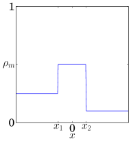
(a) Case 1.

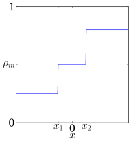
(b) Case 2.

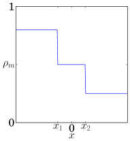
(c) Case 3.

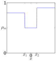
(d) Case 4.

Figure 6: Four possible cases for the initial conditions of the double Riemann problem (20).

Since the solution can contain waves whose speed becomes unbounded, it follows that we cannot solve the double Riemann problem with intermediate state $\rho_{m}$ by simply splitting the solution into two local Riemann problems and applying standard techniques. Instead, the origin and dynamics of zero waves need to be considered when constructing the solution. The double Riemann problem with a mollified flux consists of up to three separate waves. Two of the waves – which we call the 1- and 2- wave using the standard terminology – correspond respectively to the left-most ($x_{1}$) and right-most ($x_{2}$) waves arising from the initial discontinuities in the double Riemann problem. We will see later that the 1-wave is a shock and the 2-wave is a contact line. The third wave corresponds to a left-moving rarefaction wave having strength $O(\epsilon)$ and speed $O(1/\epsilon)$ that originates from the $x_{2}$ interface and is located between the other two waves. As $\epsilon\rightarrow 0$, the rarefaction wave approaches a zero wave that mediates an instantaneous interaction between the 1- and 2-waves.

4.1 Origin of Zero Waves

Since the local Riemann problem arising at the 2-wave (i.e., the contact line at the $x_{2}$ interface) is the source of the zero rarefaction wave, we begin by focusing our attention on the right half of the double Riemann problem. The formation of a zero wave at the discontinuity in the initial data located at $x_{2}$ can be divided into two cases, corresponding to whether $C_{r}<\rho_{m}$ or $C_{r}>\rho_{m}$. The specifics of the interaction between the 1-shock and the zero wave will be treated separately Section 4.2.

Zero rarefaction with $\boldsymbol{C_{r}<\rho_{m}}$ and $\boldsymbol{C_{l}=\rho_{m}}$.

We first consider the mollified Riemann problem with $C_{l}=\rho_{l}=\rho_{m}$ and $C_{r}=\rho_{r}<\rho_{m}$. The convex hull and solution profile shown in Fig. 7 exhibit a right-moving contact line (the 2-wave) having speed $s=1$ and a rarefaction wave of strength $O(\epsilon)$ travelling to the left with speed $O(1/\epsilon)$. For a simple isolated Riemann problem, the solution would reduce to a lone contact line as $\epsilon\rightarrow 0$ and the zero rarefaction would have no impact. However, when the zero wave is allowed to interact with the solution of another neighbouring Riemann problem – such as when multiple Riemann problems are solved on a sequence of grid cells in a Godunov-type numerical scheme – the local Riemann problems cannot be taken in isolation.

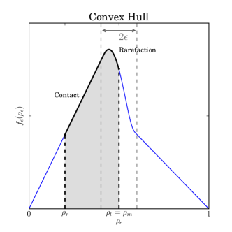
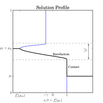
Figure 7: The convex hull (left, shaded) and solution profile (right) for the generation of the zero rarefaction wave when $\rho_{l}=\rho_{m}$ and $\rho_{r}<\rho_{m}$.

Zero rarefaction with $\boldsymbol{C_{r}>\rho_{m}}$ and $\boldsymbol{C_{l}=\rho_{m}}$.

Next we consider the mollified Riemann problem with $C_{l}=\rho_{l}=\rho_{m}$ and $C_{r}=\rho_{r}>\rho_{m}$. The convex hull and solution are depicted in Fig. 8, and the solution again consists of a contact line and zero rarefaction wave. The main difference from the previous case is that the contact line travels to the left with speed $-\gamma$ instead of to the right.

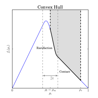
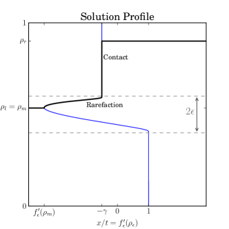
Figure 8: The convex hull (left, shaded) and solution profile (right) for the generation of the zero rarefaction wave when $\rho_{l}=\rho_{m}$ and $\rho_{r}>\rho_{m}$.

Note that since the location of the inflection point of $f_{\epsilon}(\rho_{\epsilon})$ approaches $\rho_{m}$ as $\epsilon\rightarrow 0$, an additional zero shock of strength $O(\epsilon^{2})$ and speed $O(1/\epsilon)$ is generated. For the sake of clarity, we have not included this wave in Fig. 8 since it is of higher order than the $O(\epsilon)$ zero rarefaction and so has negligible impact on the solution in the limit as $\epsilon\rightarrow 0$.

4.2 Interaction Between 1-Shock and Zero Rarefaction Wave

When solving the double Riemann problem, we need to determine how the zero rarefaction wave produced at $x_{2}$ interacts with the 1-wave, which we will see shortly must be a shock. The details of the interaction can be studied using the method of characteristics for the four cases shown in Fig. 6. Since the zero wave has speed $O(1/\epsilon)$, we must examine the shock-zero rarefaction interaction on two different time scales of length $O(\epsilon)$ and $O(1)$. Since $\lambda_{1}=O(1)$ as $\epsilon\rightarrow 0$ in each case, the problem can be simplified significantly by neglecting the shock dynamics on the $O(\epsilon)$ time scale. We will then show that the 1-wave approaches a constant speed as $\epsilon\rightarrow 0$ when $t=O(1)$.

Case 1: $\boldsymbol{C_{r},C_{l}<\rho_{m}}$.

We first consider solutions to the mollified conservation law (6) having initial conditions (20) that satisfy $C_{r},C_{l}<\rho_{m}$ as shown in Fig. 66(a). The solution in this case consists of three waves: a shock, a zero rarefaction wave, and a contact line. The initial discontinuity at $x_{2}$ generates a contact line (the 2-wave) that travels at speed $\lambda_{2}=1$, along with a zero rarefaction wave. A 1-shock originates from location $x_{1}$ and travels along the trajectory $x=S(t)$, where $S(t)$ has yet to be determined. Suppose that the zero rarefaction wave intersects the 1-wave at time $t^{*}$; then the speed of the 1-wave satisfies the Rankine-Hugoniot condition

$$\frac{dS(t)}{dt}=\lambda_{1}(t)=\frac{f_{\epsilon}(C_{l})-f_{\epsilon}(\rho_{m})}{C_{l}-\rho_{m}},\qquad\text{for\;}t\leqslant t^{*}\simeq{\mathcal{O}}(\epsilon)\mbox{.}$$ (21)

The time evolution of the solution for $t<t^{*}$ is illustrated in Fig. 99, and the corresponding plot of characteristics in the $x,t$–plane is shown in Fig. 10. The characteristics that intersect with the 1-wave for $t<t^{*}$ have speed equal to $1$ to the left of the 1-wave, and speed $O(1/\epsilon)$ to the right.

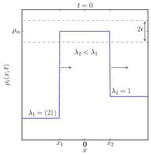
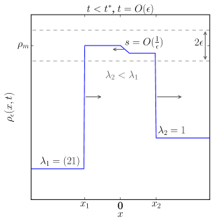
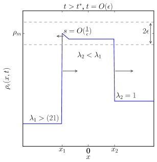
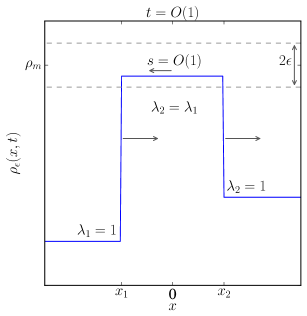
Figure 9: Time evolution of the double Riemann solution in Case 1 when $C_{r},C_{l}<\rho_{m}$. A similar picture holds in Case 4 when $C_{r},C_{l}>\rho_{m}$, except that the wave directions are reversed.

Case 1: $C_{r},C_{l}<\rho_{m}$		Case 2a: $C_{r}>\rho_{m}$ and $\gamma/(\gamma+1)\leqslant C_{l}<\rho_{m}$
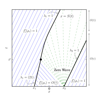
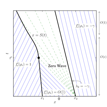
Case 2b: $C_{r}>\rho_{m}$ and $C_{l}<\gamma/(\gamma+1)<\rho_{m}$		Case 3: $C_{r}<\rho_{m}<C_{l}$

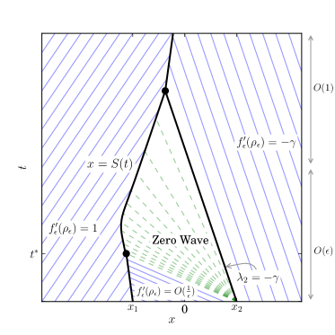
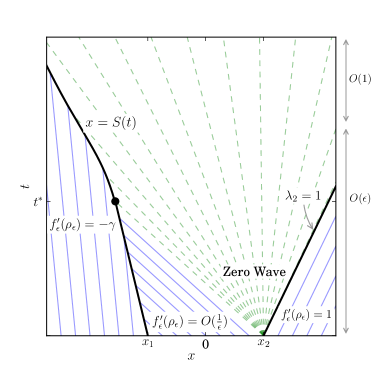
Figure 10: Characteristic lines and elementary waves in the $x,t$–plane for various cases for the double Riemann solution. The thick lines (black) represent shocks while thin lines (blue and green) represent characteristics.

At time $t^{*}$, the zero rarefaction wave starts to interact with the shock $x=S(t)$ which decreases the density $\rho_{\epsilon}$ to the right of the 1-wave as illustrated in Fig. 99. As a result, the shock wave attenuates leading to an increase in the shock speed $\lambda_{1}$. Since the zero wave contains $\rho_{\epsilon}$ values lying within the interval $[\rho_{m}-\epsilon,\rho_{m}]$, we can determine the portion of the shock–zero wave interaction that occurs on the $\epsilon$ time scale by finding the range of $\rho_{\epsilon}$ for which $f^{\prime}_{\epsilon}(\rho_{\epsilon})=O(1/\epsilon)$. Equation (9) implies that

$$f^{\prime}_{\epsilon}(\rho_{\epsilon})=O\left(\frac{1}{\epsilon}\eta\left(\frac{\rho_{\epsilon}-\rho_{m}}{\epsilon}\right)\right)\mbox{,}$$ (22)

so that we only need to determine the range of $\rho_{\epsilon}$ where

$$\eta\left(\frac{\rho_{\epsilon}-\rho_{m}}{\epsilon}\right)=O(1)\mbox{.}$$ (23)

Using the formula for the mollifier (8), it is easy to verify that (23) holds when

$$\rho_{\epsilon}=\rho_{m}+\alpha_{\epsilon}\epsilon,\qquad\lim_{\epsilon\rightarrow 0}\left(\alpha_{\epsilon}^{2}-1\right)\neq 0\qquad\text{and}\qquad\alpha_{\epsilon}\in(-1,1)\mbox{.}$$ (24)

It is only as $\rho_{\epsilon}$ approaches the boundary of the $\epsilon$-region and $\lim_{\epsilon\rightarrow 0}\left(\alpha_{\epsilon}^{2}-1\right)=0$, that $f^{\prime}_{\epsilon}(\rho_{\epsilon})=o(1/\epsilon)$. Therefore, the values of $\rho_{\epsilon}$ within the zero rarefaction wave that satisfy (24) will interact with the 1-shock on the $\epsilon$ time scale.

Because $\lambda_{1}(t)=O(1)$, we can ignore the influence of the shock over the $\epsilon$ time scale when $\epsilon\rightarrow 0$. Therefore, we only need to determine the interaction between the shock and the zero rarefaction on the $O(1)$ time scale. By finding the range of $\rho_{\epsilon}$ within the zero wave where $f^{\prime}_{\epsilon}(\rho_{\epsilon})=O(1)$, we can show that the shock speed $\lambda_{1}$ approaches a constant as $\epsilon\rightarrow 0$. By using the relationship (22), we know that there exists a $\phi$ such that $f^{\prime}_{\epsilon}(\rho_{\epsilon})=O(1)$ for all

$$\rho_{\epsilon}=\rho_{m}-\epsilon+\phi(\epsilon),$$ (25)

where $\phi(\epsilon)=o(\epsilon)$ and $\phi(\epsilon)>0$. Next, by bounding the integral

$$\displaystyle\int_{\rho_{m}-\epsilon}^{\rho_{m}-\epsilon+\phi(\epsilon)}\eta_{\epsilon}(s-\rho_{m})\,ds\leqslant~{} [\rho_{m}-\epsilon+\phi(\epsilon)-(\rho_{m}-\epsilon)]\eta_{\epsilon}(\rho_{m}-\epsilon+\phi(\epsilon)-\rho_{m}),$$

$$=~{} \phi(\epsilon)\eta_{\epsilon}(-\epsilon+\phi(\epsilon)),$$

$$=~{} O(\phi(\epsilon))\mbox{,}$$

we know from Eq. (7) that

$$f_{\epsilon}(\rho_{\epsilon})=\rho_{\epsilon}+O(\phi(\epsilon)),$$

for the range of $\rho_{\epsilon}$ defined by Eqs. (25). Therefore, as $\epsilon\rightarrow 0$, we have that $f_{\epsilon}(\rho_{\epsilon})\rightarrow g_{f}(\rho_{m})$ and the shock speed $\lambda_{1}\rightarrow 1$. This results in a solution of the form

$$\rho(x,t)=\left\{\begin{array}[]{ll}C_{l},&\text{if}~{}x<x_{1}+\lambda_{1}t,\\ \rho_{m},&\text{if}~{}x_{1}+\lambda_{1}t\leqslant x\leqslant x_{2}+\lambda_{2}t,\\ C_{r},&\text{if}~{}x>x_{2}+\lambda_{2}t,\end{array}\right.$$ (26)

where $\lambda_{1}=\lambda_{2}=1$. Therefore, at longer times the solution takes the form of a “square wave” propagating to the right at constant speed as pictured in Fig. 99.

Case 2: $\boldsymbol{C_{l}<\rho_{m}<C_{r}}$.

Next, we consider the double Riemann problem when $C_{r}>\rho_{m}$ and $C_{l}<\rho_{m}$ which generates a zero rarefaction wave and contact line at $x_{2}$, and a shock at $x_{1}$. Before the 1-shock and zero rarefaction wave interact at time $t^{*}=O(\epsilon)$, the shock speed $\lambda_{1}$ satisfies the Rankine-Hugoniot condition (21). For $t>t^{*}$, the shock and zero rarefaction interact, thereby causing the value of $\rho_{\epsilon}$ to the right of the 1-wave to increase. Using a similar argument as in Case 1, we can deduce that when $t=O(1)$,

$$\lambda_{1}=\frac{g_{c}(\rho_{m})-f(C_{l})}{\rho_{m}-C_{l}}\qquad\text{and}\qquad\lambda_{2}=-\gamma,$$ (27)

as $\epsilon\rightarrow 0$. Note that these wave speeds are consistent with the Riemann problem in Eq. (17). The time evolution of the solution is illustrated in Fig. 11.

There are actually two distinct sub-cases that need to be considered here, corresponding to whether $C_{l}\geqslant\gamma/(\gamma+1)$ (which we call Case 2a) or $C_{l}<\gamma/(\gamma+1)$ (Case 2b). In Case 2a, the two elementary waves (1–shock and 2–contact) do not interact, while in Case 2b we have $\lambda_{1}>\lambda_{2}$ and so the elementary waves collide to form a single shock that has speed given by Eq. (19). This distinction is illustrated in the characteristic plots in Fig. 10.

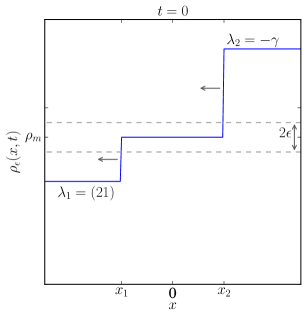
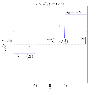
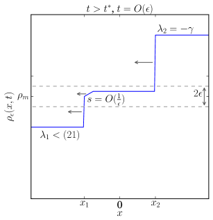
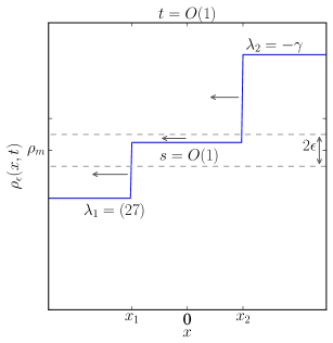
Figure 11: Time evolution of the double Riemann solution in Case 2a when $C_{r}>\rho_{m}$ and $\gamma/(\gamma+1)\leqslant C_{l}<\rho_{m}$.

Case 3: $\boldsymbol{C_{r}<\rho_{m}<C_{l}}$.

We next consider the situation when $C_{r}<\rho_{m}<C_{l}$, where a zero rarefaction wave and contact line are produced at $x_{2}$ and a shock wave is generated at $x_{1}$. Before the 1-shock and zero rarefaction wave interact at time $t^{*}=O(\epsilon)$, the shock speed $\lambda_{1}$ satisfies the Rankine-Hugoniot condition (21) as illustrated in Figs. 1212 and 12. Once the zero wave collides with the shock, the shock speed $\lambda_{1}$ increases according to the Rankine-Hugoniot condition since the value of $\rho_{\epsilon}$ to the right of the 1-wave decreases (shown in Fig. 1212). By ignoring interactions on the $O(\epsilon)$ time scale, we find that

$$\lambda_{1}=\frac{g_{f}(\rho_{m})-f(C_{l})}{\rho_{m}-C_{l}},\qquad\text{and}\qquad\lambda_{2}=1,$$ (28)

for $t=O(1)$ as $\epsilon\rightarrow 0$. Notice that the wave speeds $\lambda_{1}$ and $\lambda_{2}$ are identical to those for the Riemann problem considered in Case C from Section 3.

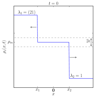
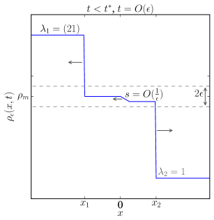
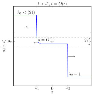
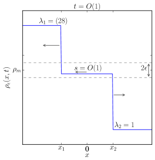
Figure 12: Time evolution of the double Riemann solution in Case 3 when $C_{r}<\rho_{m}<C_{l}$.

Case 4: $\boldsymbol{C_{r},C_{l}>\rho_{m}}$.

The final remaining case corresponds to $C_{r},C_{l}>\rho_{m}$ and leads to a solution satisfying Eq. (26) with

$$\lambda_{1}=\frac{g_{c}(\rho_{m})-f(C_{l})}{\rho_{m}-C_{l}}\qquad\text{and}\qquad\lambda_{2}=-\gamma.$$ (29)

The speed of the 1-shock is determined simply by the Rankine-Hugoniot condition where $f(\rho_{m})$ is evaluated on the congested flow branch. This should be compared to the 1-wave in Case 3 where the shock speed is determined by Eq. (28) in which $f(\rho_{m})$ is evaluated on the free flow branch. No plots of the solution have been provided for Case 4 since the structure is essentially the same as in Case 1 except that all waves propagate in the opposite direction.

5 Finite Volume Scheme of Godunov Type

In this section, we construct a finite volume scheme of Godunov type for our discontinuous flux problem based on ideas originally developed by Godunov [18] for solving the Euler equations of gas dynamics. In Godunov’s method, the spatial domain is divided into cells $[x_{j-1/2},x_{j+1/2}]$ of constant width, $\Delta x=x_{j+1/2}-x_{j-1/2}$, and the solution is assumed to be piecewise constant on each grid cell. Cell-averaged solution values $Q_{j}^{n}$ (located at cell centers) are updated using the exact solution from local Riemann problems evaluated at interfaces between adjacent cells. In each time step, the following three-stage algorithm, referred to as the Reconstruct–Evolve–Average or REA algorithm in [28], is used to update the $Q_{j}^{n}$:

• Reconstruct a piecewise constant function $\tilde{\rho}(x,t_{n})=Q_{j}^{n}$ for all $x\in[x_{j+1/2},x_{j-1/2}]$ from the cell average $Q_{j}^{n}$ at time $t_{n}$.

• Evolve the conservation law exactly using initial data $\tilde{\rho}(x,t_{n})$, thereby obtaining $\tilde{\rho}(x,t_{n+1})$ at time $t_{n+1}=t_{n}+\Delta t$.

• Average the solution $\tilde{\rho}(x,t_{n+1})$ to obtain new cell average values

  $$Q_{j}^{n+1}=\frac{1}{\Delta x}\int_{x_{j-1/2}}^{x_{j+1/2}}\tilde{\rho}(x,t_{n+1})\,dx\mbox{.}$$

For problems with smooth flux, the evolution step can be performed by solving a local Riemann problem at each cell interface having left state $\rho_{l}=Q_{j}^{n}$ and right state $\rho_{r}=Q_{j+1}^{n}$. As long as the time step is chosen small enough, the elementary waves produced at each interface do not interact (remembering that waves travel at finite speed in the smooth case) and hence the evolution step yields an appropriate approximation of the solution. However, as we have already shown, when the flux is discontinuous the presence of zero waves travelling at infinite speed gives rise to long-range interactions between local Riemann problems. Consequently, we make use of solutions to the double Riemann solution derived in the previous section that incorporate the effects of zero waves. We note that the resulting algorithm has some similarities to the method of Gimse [16].

We next provide details of our implementation using LeVeque’s high resolution wave propagation formulation [28], in which the Riemann solver returns a set of wave strengths $\mathcal{W}^{p}_{j+1/2}$ and speeds $s^{p}_{j+1/2}$ generated at each interface between states $Q_{j}$ and $Q_{j+1}$ (in what follows, we will omit the superscript $n$ when it is clear that time index $n$ is assumed). The evolution step of the algorithm above can then be written as

$$Q_{j}^{n+1}=Q_{j}^{n}-\frac{\Delta t}{\Delta x}\left[\sum_{p}\left(s_{j-1/2}^{p}\right)^{+}\mathcal{W}_{j-1/2}^{p}+\sum_{p}\left(s_{j+1/2}^{p}\right)^{-}\mathcal{W}_{j+1/2}^{p}\right],$$ (30)

where $(s)^{+}=\max(s,0)$ and $(s)^{-}=\min(s,0)$. When the flux is smooth, the wave speed $s_{j+1/2}$ depends only on the states $Q_{j}$ and $Q_{j+1}$, whereas for a discontinuous flux function this is no longer the case. When $Q_{j},Q_{j+1}\neq\rho_{m}$, the Riemann solver yields the “standard” elementary waves whose strength and speed are given in Section 3. Because our flux is strictly non-convex, we also observe compound waves which are described within Cases 1 and 2 in Section 3.

Our Riemann problem solution diverges from the standard one when either $Q_{j}=\rho_{m}$ or $Q_{j+1}=\rho_{m}$, in which case we construct the solution to a local double Riemann problem that requires the appropriate 1- or 2-wave given in Section 4. Note that the double Riemann solution should be viewed as two separate local Riemann problems that each produce one elementary wave: the left Riemann problem corresponds to the 1-wave and the right Riemann problem corresponds to the 2-wave.

For example, if $Q_{j}=\rho_{m}$, then we construct the double Riemann problem with $Q_{j}=\rho_{m}$ and $Q_{j+1}=C_{r}$, thereby obtaining the strength and wave speed corresponding to the 2-wave in Section 4. Combining together all four cases in Section 4.2, the speed can be written as

$$s^{1}_{j+1/2}=\left\{\begin{array}[]{ll}1~{},&~{}Q_{j+1}<\rho_{m}\\ -\gamma~{},&~{}Q_{j+1}>\rho_{m}\end{array}\right.\mbox{,}$$ (31)

which we note is independent of $C_{l}$.

Alternatively, if $Q_{j+1}=\rho_{m}$ then we construct the double Riemann problem with $Q_{j}=C_{l}$, $Q_{j+1}=\rho_{m}$ and unknown $Q_{I}=C_{r}$, thereby obtaining the strength and wave speed for the 1-wave in Section 4. In contrast with the case $Q_{j}=\rho_{m}$ just considered, the 1-wave’s speed depends on values of $C_{l}$, $\rho_{m}$, and $C_{r}$. Therefore, when determining the speed of the wave at the interface between $Q_{j}=C_{l}$ and $Q_{j+1}=\rho_{m}$, we must look ahead to find the value $Q_{I}=C_{r}$ corresponding to the first value of $Q_{j}$ not equal to $\rho_{m}$; that is,

$$I=\min\left\{~{}k~{}|~{}j+1<k\leqslant N\mbox{ and }Q_{k}\neq\rho_{m}\right\}.$$ (32)

In summary, when $Q^{n}_{j+1}=\rho_{m}$, the wave speed reduces to

$$s^{1}_{j+1/2}=\left\{\begin{array}[]{ll}\displaystyle\frac{g_{f}(\rho_{m})-f(Q_{j})}{\rho_{m}-Q_{j}}~{},&~{}Q_{I}<\rho_{m}\\ \displaystyle\frac{g_{c}(\rho_{m})-f(Q_{j})}{\rho_{m}-Q_{j}}~{},&~{}Q_{I}>\rho_{m}\end{array}\right.$$ (33)

which is visualized in Fig. 13.

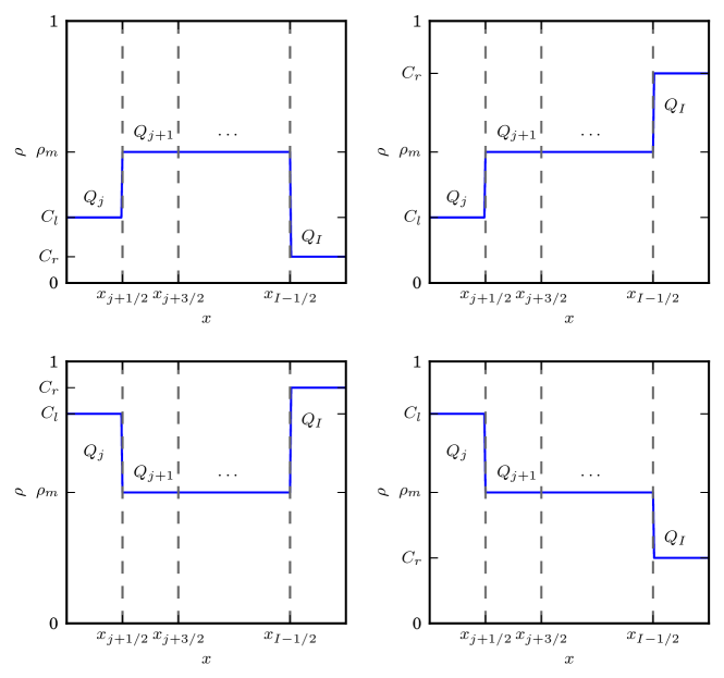
Figure 13: The four possible cases that can arise when calculating the shock speed in Eq. (33).

Note that we have not yet discussed the two simple cases when $Q_{j},Q_{j+1}<\rho_{m}$ and $Q_{j},Q_{j+1}>\rho_{m}$, both of which reduce to the linear advection equation and can be trivially solved. A summary of wave strengths and speeds for all cases is presented in Table 1.

Table 1: Wave speed and strength for the 1- and 2-waves in all possible cases.

Case		$s^{1}_{j+1/2}$	$\mathcal{W}^{1}_{j+1/2}$	$s^{2}_{j+1/2}$	$\mathcal{W}^{2}_{j+1/2}$
	$Q_{j}=Q_{j+1}=\rho_{m}$	$0$	$0$	$0$	$0$
	$Q_{j}=\rho_{m}$ and $Q_{j}\neq Q_{j+1}$	Eq. (31)	$Q_{j+1}-Q_{j}$	$0$	$0$
	$Q_{j+1}=\rho_{m}$ and $Q_{j}\neq Q_{j+1}$	Eq. (33)	$Q_{j+1}-Q_{j}$	$0$	$0$
	$\rho_{m}<Q_{j}$ and $\rho_{m}<Q_{j+1}$	$-\gamma$	$Q_{j+1}-Q_{j}$	$0$	$0$
	$\rho_{m}>Q_{j}$ and $\rho_{m}>Q_{j+1}$	$1$	$Q_{j+1}-Q_{j}$	$0$	$0$
	$Q_{j}<\rho_{m}<Q_{j+1}$ and $\displaystyle\frac{\gamma}{\gamma+1}\geqslant Q_{j}$	$\displaystyle\frac{f(Q_{j+1})-f(Q_{j})}{Q_{j+1}-Q_{j}}$	$Q_{j+1}-Q_{j}$	$0$	$0$
	${\displaystyle\frac{\gamma}{\gamma+1}}<Q_{j}<\rho_{m}<Q_{j+1}$	$-\gamma$	$Q_{j+1}-\rho_{m}$	$\displaystyle\frac{g_{c}(\rho_{m})-f(Q_{j})}{\rho_{m}-Q_{j}}$	$\rho_{m}-Q_{j}$
	$Q_{j+1}<\rho_{m}<Q_{j}$	$\displaystyle\frac{f(Q_{j})-g_{f}(\rho_{m})}{Q_{j}-\rho_{m}}$	$\rho_{m}-Q_{j}$	$1$	$Q_{j+1}-\rho_{m}$

A slight modification to the local Riemann solver is required to deal with the fact that algebraic operations are actually performed in floating-point arithmetic. It is highly unlikely that the numerical value of $Q_{j}$ ever exactly equals $\rho_{m}$, and yet we find that it is necessary to employ the solution of the double Riemann problem when $Q_{j}$ is close to $\rho_{m}$. Therefore, we need to relax the requirement slightly for the zero-wave cases by replacing the condition $Q_{j}=\rho_{m}$ with

$$|Q_{j}-\rho_{m}|\leqslant\delta\mbox{,}$$ (34)

where $\delta$ is a small parameter that is typically assigned values on the order of $10^{-5}$. The choice of $\delta$ is a balance between accuracy and efficiency in that taking a larger $\delta$ value gives rise to significant deviations in the height of the $\rho_{m}$ plateau regions, and hence also errors in mass conservation. Taking $\delta$ values much smaller than $10^{-5}$ does not improve the solution significantly but does require a smaller time step for stability. This modification influences the accuracy of the simulations and also creates an artificial upper bound on the maximum wave speed, not including zero waves. For example, consider the shock solution in Eq. (17), where as $\rho_{l}$ approaches $\rho_{m}$ the shock speed becomes unbounded. By enforcing (34), the parameter $\delta$ determines how close $\rho_{l}$ can be to $\rho_{m}$ before the algorithm switches to the double Riemann solution.

The time step $\Delta t$ is chosen adaptively to enforce stability of our explicit update scheme, using a restriction based on the wave speeds from all local Riemann problems. In particular, we take

$$\Delta t=\mbox{{CFL}}\cdot\min_{j,p}\left(\frac{\Delta x}{|s^{p}_{j+1/2}|}\right),$$

where $0<\mbox{{CFL}}<1$ is a constant chosen to be around 0.9 in practice. As long as the parameter $\delta$ is not taken too small, this condition is sufficient to guarantee stability. Because the effects of the zero waves have been incorporated directly into the Riemann problem, they have no direct influence on the stability restriction.

The Riemann solver described above forms the basis for the first-order Godunov scheme. We have also implemented a high resolution variant using wave limiters which limit the waves $\mathcal{W}^{p}_{j+1/2}$ in a manner similar to the limiting of fluxes in flux-based finite volume schemes. The details of this modification are described in [28].

6 Numerical Results

We now apply the method described in the previous section to a number of test problems. For the high resolution scheme, we employ the superbee limiter function. In all cases, we use the discontinuous, piecewise linear flux function (3)–(4) with parameters $\rho_{m}=0.5$ and $\gamma=0.5$ that is pictured in Fig. 14.

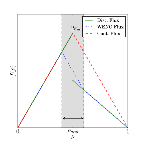
Figure 14: Plots of the discontinuous flux function used in our high resolution simulations (with $\rho_{m}=0.5$, $\gamma=0.5$), the regularized flux for WENO calculations in Section 6.2, and the continuous flux used in Section 6.3.

6.1 Riemann Initial Data

As a first illustration of our numerical method, we use three sets of Riemann initial data:

1. $\rho_{l}=0.9$ and $\rho_{r}=0.2$,

2. $\rho_{l}=0.4$ and $\rho_{r}=0.9$,

3. $\rho_{l}=0.3$ and $\rho_{r}=0.98$,

for which the exact solution can be determined using the methods in Sections 3 and 4. These initial data labeled A, B and C correspond to the three “Cases” with the same labels in Section 3 and pictured in Figs. 3, 4 and 5 respectively. We note that the numerical values for the left and right states in Case C differ slightly from the initial data used in Fig. 5 in order to generate larger wave speeds.

In Fig. 15 (left), we compare the results from the first order Godunov method and the high resolution scheme with wave limiters. In each case, we perform a convergence study of error in the discrete L1 norm for grid resolutions ranging from $\Delta x=0.05$ to $0.0025$. Convergence rates estimated using a linear least squares fit are summarized in Table 2. As expected, the numerical scheme converges to the exact solution for all three test problems.  Godunov’s method captures the correct speed for both the shock and contact discontinuities, although there is a more noticeable smearing of the contact line which is typical for this type of problem. The L1 convergence rates are consistent with the order $\sqrt{\Delta x}$ spatial error estimate established analytically for discontinuous solutions of hyperbolic conservation laws having a smooth flux [26, 32]. The convergence rates in the L2 norm are also provided for comparison purposes and are significantly smaller than the corresponding L1 rates, as expected.

Table 2: Convergence rates for the three Riemann problems pictured in Fig. 15.

			Godunov		High Resolution
$\rho_{l}$	$\rho_{r}$		L1	L2	L1	L2
${0.9}$	${0.2}$		$0.643$	$0.367$	$1.022$	$0.569$
${0.4}$	${0.9}$		$0.488$	$0.232$	$0.832$	$0.375$
${0.3}$	${0.98}$		$0.754$	$0.373$	$1.053$	$0.627$
${0.1}$	${0.4}$		$0.487$	$0.145$	$0.700$	$0.238$

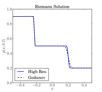
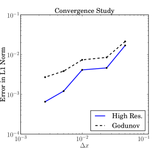
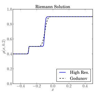
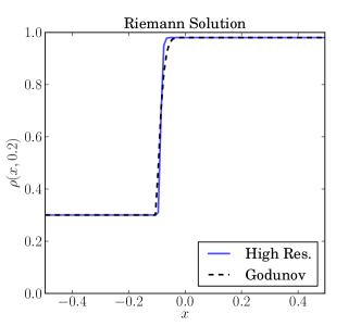
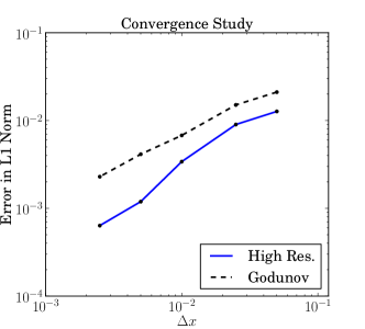
Figure 15: Left: Computed solutions for the Riemann initial data at $t=0.2$ where $\delta=10^{-7}$, $\Delta x=0.01$, $\mbox{CFL}=0.95$, $\rho_{m}=0.5$, and $\gamma=0.5$. Right: Convergence study in the L1 norm.

6.2 Smooth Initial Data, With WENO Comparison

For the next series of simulations, we use the smooth initial data

$$\rho(x,0)=\exp\left(-\frac{x^{2}}{2\sigma^{2}}\right),$$ (35)

where $\sigma=0.1$ and the domain is the interval $[-1,1]$ with periodic boundary conditions. This corresponds in the traffic flow context to a single platoon of cars travelling on a ring road, where the initial density peak has a maximum value of 1 and decreases smoothly to zero on either side. Fig. 16 depicts the time evolution of the solution computed using our high resolution Godunov scheme. Initially, the platoon begins to spread out and a horizontal plateau appears on the right side at a value of $\rho=\rho_{m}$. This plateau value corresponds to the “optimal” traffic density that is the maximum value of $\rho$ for which cars can still propagate at the free-flow speed. The plateau lengthens as a shock propagates to the left into the upper half of the density profile, reducing the width of the peak. At the same time, the cars in the dense region spread out to the right as the plateau also extends in the same direction, while the left edge of the platoon remains essentially stationary until the dense peak is entirely gone. When the peak finally disappears (near time $t=0.18$), the remaining platoon of cars propagates to the right with constant speed and unchanged shape. Note that the traffic density evolves such that the area under the solution curve remains approximately constant, since the total number of cars must be conserved.

For comparison purposes, we have also performed simulations using the WENO scheme in CentPack [2], which employs a third-order CWENO reconstruction in space [25, 29] and a third-order SSP Runge-Kutta time integrator [19]. Because this algorithm requires the flux function to be continuous (although not smooth), we have used a regularized version of the flux that is piecewise linear and continuous, replacing the discontinuity by a steep line segment connecting the two linear pieces over a narrow interval of width $2\epsilon_{w}$ (instead of using the function $f_{\epsilon}$ in (7) because that would require an integral to be evaluated for every flux function evaluation). The regularized flux is shown in Fig. 14.

From Fig. 16, we observe that the WENO simulation requires a substantially smaller time step and grid spacing in order to obtain results that are comparable to our method. In particular, the WENO scheme requires a time step of $\Delta t=O(10^{-6})$ and a spatial resolution of $\Delta x=O(10^{-4})$ when $\epsilon_{w}=10^{-3}$; this can be compared with our high resolution Godunov scheme for which we used a time step of $\Delta t=O(10^{-4})$ when $\Delta x=O(10^{-3})$ and $\delta=10^{-5}$. This performance difference is magnified further as $\epsilon_{w}$ decreases due to the ill-conditioning of the regularized-flux problem.

In Fig. 17, we magnify the region containing the density peak at time $t=0.1$ to more easily visualize the difference between the two sets of results for different values of $\epsilon_{w}$ and $\delta$. From these plots we observe that the two solutions approach one another as both $\epsilon_{w}$ and $\delta$ are reduced, which provides further evidence that our high resolution Godunov scheme computes the correct solution. Note that the WENO scheme does yield a slightly sharper resolution of the shock than our method, but on the other hand it significantly underestimates the height of the plateau region when $\epsilon_{w}$ is too large.

Next, we estimate the error in our high resolution Godunov scheme by comparing the computed solutions on a sequence of successively finer grids with $\Delta x_{p}=\Delta x_{0}/3^{p}$ for $p=0,1,\ldots,P$, with $P=6$ levels of refinement. The finest grid solution with $\Delta x=\Delta x_{P}$ is treated as the “exact” solution for the purposes of this convergence study. The errors at $t=0.05$ shown in Fig. 1818 exhibit convergence rates of approximately 1.125 in the L1 norm and 0.632 in the L2 norm which are consistent with the results from Section 6.1. We note that even though the initial data are smooth, our high resolution Godunov scheme does not obtain second order accuracy because of the shock that appears immediately on the right side of the plateau.

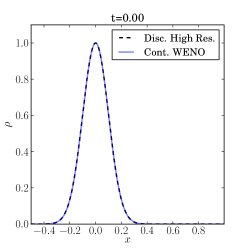
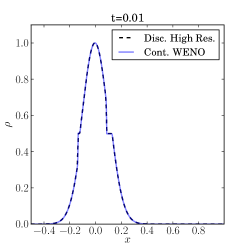
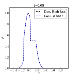
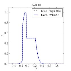
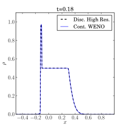
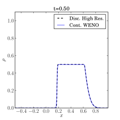
Figure 16: Time evolution of the solution with smooth initial conditions using a high resolution scheme ($\delta=10^{-5}$, $\Delta x=0.005$, $\mbox{CFL}=0.9$) and a third-order WENO scheme [2] ($\Delta x=0.0004$, $\epsilon_{w}=10^{-3}$, $\mbox{CFL}=0.9$) where $\rho_{m}=0.5$ and $\gamma=0.5$.

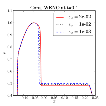
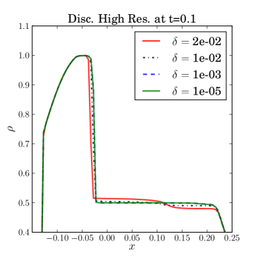
Figure 17: 17 WENO simulation for different $\epsilon_{w}$ for problem pictured in Fig. 16 where $\Delta x=0.0004$ and $\Delta t=O(10^{-6})$). 17 High resolution simulation for different $\delta$ for problem pictured in Fig. 16 where $\Delta x=0.005$ and $\Delta t=O(10^{-4})$).

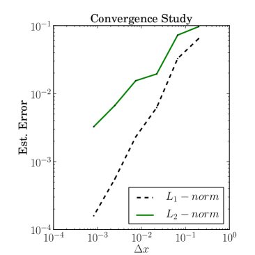
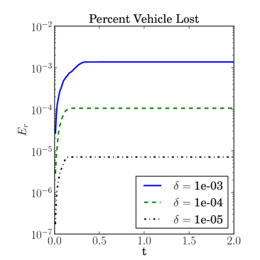
Figure 18: 18 Convergence study for the problem with smooth initial data at $t=0.05$ using $\Delta x_{0}=0.2$ and $P=6$ levels of refinement (refer to Fig. 16). 18 Percentage of the initial vehicles lost during the simulation using different $\delta$ values.

Because convergence rates provide only a rough measure of solution error, we can gain additional insight into the accuracy of the method by measuring conservation error, which is expressed in terms of the variation $V$ in the total number of vehicles via

$$E_{r}=\frac{V^{n}-V^{0}}{V^{0}}\quad\text{where}\quad V^{n}=\Delta x\sum_{j=1}^{N}Q_{j}^{n}.$$

Since we are using periodic boundary conditions and have no external sources or sinks, $V^{n}$ should remain approximately constant for all $n$. Indeed, Fig. 1818 shows that the numerical scheme accumulates only a small conservation error over time, and that the rate of vehicles lost can be controlled by reducing $\delta$.

6.3 Smooth Initial Data, With Continuous Flux Comparison

In this final set of simulations, we compare solutions of the conservation law (3) with the discontinuous piecewise linear flux (4) and the continuous piecewise linear flux

$$f_{c}(\rho)=\left\{\begin{array}[]{ll}\displaystyle\rho,&\text{if}~{}0\leqslant\rho<\rho_{m},\\ \displaystyle\frac{\rho_{m}}{1-\rho_{m}}(1-\rho),&\text{if}~{}\rho_{m}\leqslant\rho\leqslant 1.\end{array}\right.$$ (36)

Both fluxes are illustrated in Fig. 14.

We begin by emphasizing that these two seemingly very different flux functions can still give rise to similar solutions to the Riemann problem with suitably chosen piecewise constant initial data. For Cases A and C from Section 3, the convex hulls and the corresponding solutions are identical for the two fluxes. However, the convex hulls are different in Case B, where the discontinuous flux gives rise to the compound wave illustrated in Fig. 4 while the continuous flux generates a single shock (analogous to the solution in Fig. 5). Furthermore, the continuous flux (36) does not give rise to any zero waves; instead, when either $\rho_{l}=\rho_{m}$ or $\rho_{r}=\rho_{m}$, a single contact line is produced that satisfies the Rankine-Hugoniot condition.

A clear illustration of the difference between these two fluxes is provided by comparing simulations on the periodic domain $x\in[-1,1]$ for smooth initial data

$$\rho(x,0)=\frac{1}{2}\exp\left(-\frac{x^{2}}{2\sigma^{2}}\right)+\frac{2}{5},$$ (37)

where $\sigma=0.1$. This corresponds to the situation where there is a Gaussian-shaped congestion in the middle of free-flow traffic on a ring road.

Fig. 19 depicts the time evolution of the solution computed using a high resolution Godunov scheme for the continuous and discontinuous fluxes. Note that the numerical solution for the discontinuous flux requires application of the look-ahead procedure discussed in Section 5 while the continuous flux requires only the calculation of interactions between adjacent cells. Initially, the congested region begins to spread out and a horizontal plateau appears on the right side at a value of $\rho=\rho_{m}$. On the left edge of this plateau, a shock appears for the discontinuous flux in comparison with a gradual continuous variation in density for the continuous flux.

The solutions are more drastically different when comparing the dynamics on the left edge of the congested region. For the discontinuous flux, a compound wave forms to the left of the peak, resulting in the formation of a second horizontal plateau at the maximum congested flow speed $\rho=\rho_{m}$. Therefore, drivers on the far left will enter into a optimal congested flow before being hit by the left-moving congestion wave. The continuous flux, on the other hand, produces only a single left-moving congestion wave.

We conclude therefore that if the fundamental diagram is discontinuous, we expect to observe compound congestion waves. The leading congestion wave acts to push vehicles into some form of optimal congested flow, possibly a synchronized traffic state. This wave is followed up by a slower congestion wave. Note that we only expect these compound congestion waves when the upstream free flow traffic has sufficiently high density. For example, in Fig. 16, we observed only a single congestion shock because the traffic density to the left is too small to sustain this compound congestion wave.

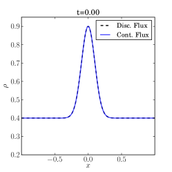
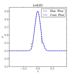
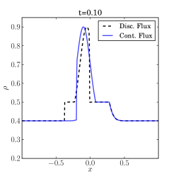
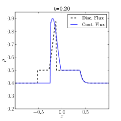
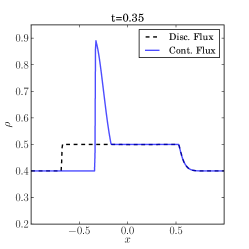
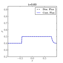
Figure 19: Time evolution of the solution with smooth initial conditions using a high resolution scheme ($\delta=10^{-5}$, $\Delta x=0.005$, $\mbox{CFL}=0.9$) for both the smooth and discontinuous flux.

7 Conclusions

In this paper, we derived analytical solutions to the Riemann problem for a hyperbolic conservation law with a piecewise linear flux function having a discontinuity at the point $\rho=\rho_{m}$. In the case when the left and right states in the Riemann initial data lie on either side of the discontinuity, the solution consists of a compound wave made up of a shock and contact line connected by a constant intermediate state at $\rho_{m}$. In the special case when either the left or right state equals $\rho_{m}$, the Riemann problem gives rise to a zero rarefaction wave that propagates with infinite speed. Even though the strength of this wave is zero, it nonetheless has a significant impact on the solution structure as it interacts with other elementary waves.

Our analytical results were validated using a high resolution Godunov-type scheme, based on our exact Riemann solver and implemented using the wave propagation formalism of LeVeque [28]. This approach builds the effect of zero waves directly into the algorithm in a way that avoids the overly stringent CFL time step constraint that might otherwise derive from the infinite speed of propagation of zero waves. We demonstrate the accuracy and efficiency of our method using several test problems, and include comparisons with higher-order WENO simulations.

We conclude with a brief discussion of several possible avenues for future research. First, a detailed convergence analysis of the algorithm would help to identify non-smooth error components that arise from the discontinuity in the flux, as well as the look-ahead procedure required to determine shock speeds in the case when $\rho_{m}=\rho_{l}$ or $\rho_{r}$. Second, we would like to consider other nonlinear forms of the piecewise discontinuous flux function since the linearity assumption in this paper simplifies our analytical solutions considerably in that elementary waves arising from local Riemann problems consist of shocks and contact lines only. For example, it would be interesting to perform a detailed comparison with the results of Lu et al. [31] who considered a discontinuous, piecewise quadratic flux. Thirdly, we mention some preliminary computations of traffic flow using a cellular automaton model [37] that give rise to an apparent discontinuity in the fundamental diagram. This connection between cellular automaton models (that only specify rules governing individual driver behaviour) and kinematic wave models (in which the two-capacity effect is incorporated explicitly via the flux function) merits further study. Finally, the situation where the flux is a discontinuous function of the spatial variable has been analyzed much more extensively (see the journal issue introduced by the article [6], and references therein). We would like to draw deeper connections between this work and the problem where the discontinuity appears in the density.

References

- [1] D. Armbruster, S. Göttlich, and M. Herty. A scalar conservation law with discontinuous flux for supply chains with finite buffers. SIAM J. Appl. Math., 71(4):1070–1087, 2011.
- [2] J. Balbas and E. Tadmor. CentPack. Available on-line at http://www.cscamm.umd.edu/centpack/software, July 2006.
- [3] J. H. Bank. Two-capacity phenomenon at freeway bottlenecks: a basis for ramp metering. Transp. Res. Rec., 1320:83–90, 1991.
- [4] J. H. Bank. The two-capacity phenomenon: some theoretical issues. Transp. Res. Rec., 1320:234–241, 1991.
- [5] R. Bürger, A. García, K. H. Karlsen, and J. D. Towers. Difference schemes, entropy solutions, and speedup impulse for an inhomogeneous kinematic traffic flow model. Netw. Heterog. Media, 3(1):1–41, 2008.
- [6] R. Bürger and K. H. Karlsen. Conservation laws with discontinuous flux: A short introduction. J. Engrg. Math., 60(3):241–247, 2008.
- [7] A. Ceder. A deterministic traffic flow model for the two-regime approach. Transp. Res. Rec., 567:16–30, 1976.
- [8] R. M. Colombo. Hyperbolic phase transitions in traffic flow. SIAM J. Appl. Math., 63(2):708–721, 2002.
- [9] C. F. Daganzo. Requiem for second-order fluid approximations of traffic flow. Transp. Res. B, 29(4):277–286, 1995.
- [10] J. P. Dias and M. Figueira. On the Riemann problem for some discontinuous systems of conservation laws describing phase transitions. Commun. Pure Appl. Anal., 3:53–58, 2004.
- [11] J. P. Dias and M. Figueira. On the approximation of the solutions of the Riemann problem for a discontinuous conservation law. Bull. Braz. Math. Soc., 36(1):115–125, 2005.
- [12] J. P. Dias and M. Figueira. On the viscous Cauchy problem and the existence of shock profiles for a p-system with a discontinuous stress function. Quart. Appl. Math., 63(2):335–341, 2005.
- [13] J. P. Dias, M. Figueira, and J. F. Rodrigues. Solutions to a scalar discontinuous conservation law in a limit case of phase transitions. J. Math. Fluid Mech., 7(2):153–163, 2005.
- [14] S. M. Easa. Selecting two-regime traffic-flow models. Transp. Res. Rec., 869:25–36, 1982.
- [15] L. C. Edie. Car-following and steady-state theory for noncongested traffic. Opns. Res., 9(1):66–76, 1961.
- [16] T. Gimse. Conservation laws with discontinuous flux functions. SIAM J. Math. Anal., 24(2):279–289, 1993.
- [17] P. Goatin. The Aw-Rascle vehicular traffic flow model with phase transitions. Math Comput. Model., 44(3–4):287–303, 2006.
- [18] S. K. Godunov. A difference method for numerical calculation of discontinuous solutions of the equations of hydrodynamics. Mat. Sb., 47:271–306, 1959.
- [19] S. Gottlieb, C. W. Shu, and E. Tadmor. Strong stability-preserving high-order time discretization methods. SIAM Rev., 43(1):89–112, 2001.
- [20] B. D. Greenshields. A study of traffic capacity. Proc. Highw. Res., 14(1):448–477, 1935.
- [21] F. L. Hall, B. L. Allen, and M. A. Gunter. Empirical analysis of freeway flow-density relationships. Transp. Res. A, 20(3):197–210, 1986.
- [22] D. Helbing. Traffic and related self-driven many-particle systems. Rev. Mod. Phys., 73:1067–1141, 2001.
- [23] B. S. Kerner. The Physics of Traffic: Empirical Freeway Pattern Features, Engineering Applications and Theory. Springer, 2004.
- [24] M. Koshi, M. Iwasaki, and I. Ohkura. Some findings and an overview on vehicular flow characteristics. In V. F. Hurdle, E. Hauer, and G. N. Steuart, editors, Proceedings of the Eighth International Symposium on Transportation and Traffic Theory, pages 403–426, Toronto, Canada, June 24–26, 1981. University of Toronto Press.
- [25] A. Kurganov and D. Levy. A third-order semi-discrete central scheme for conservation laws and convection-diffusion equations. SIAM J. Sci. Comput., 22(4):1461–1488, 2000.
- [26] N. N. Kuznetsov. Accuracy of some approximate methods for computing the weak solutions of a first-order quasi-linear equation. USSR Comput. Math. Math. Phys., 16(6):105–119, 1976.
- [27] R. J. LeVeque. Some traffic flow models illustrating interesting hyperbolic behavior. In Minisymposium on traffic flow, SIAM Annual Meeting, July 10, 2001. Available on-line at http://faculty.washington.edu/rjl/pubs/traffic/traffic.pdf.
- [28] R. J. LeVeque. Finite Volume Methods for Hyperbolic Problems. Cambridge University Press, New York, 2002.
- [29] D. Levy, G. Puppo, and G. Russo. Central WENO schemes for hyperbolic systems of conservation laws. Math. Model. Numer. Anal., 33:547–571, 2001.
- [30] M. J. Lighthill and G. B. Whitham. On kinematic waves. II. A theory of traffic flow on long crowded roads. Proc. Roy. Soc. Lond. A, 229(1178):317–345, 1955.
- [31] Y. Lu, S. C. Wong, M. Zhang, and C.-W. Shu. The entropy solutions for the Lighthill-Whitham-Richards traffic flow model with a discontinuous flow-density relationship. Transp. Sci., 43(4):511–530, 2009.
- [32] B. J. Lucier. Error bounds for the methods of Glimm, Godunov and LeVeque. SIAM J. Numer. Anal., 22(6):1074–1081, 1985.
- [33] S. Martin and J. Vovelle. Convergence of implicit finite volume methods for scalar conservation laws with discontinuous flux function. Math. Model. Numer. Anal., 42(5):699–727, 2008.
- [34] O. Oleĭnik. Uniqueness and stability of the generalized solution of the Cauchy problem for a quasilinear equation. Amer. Math. Soc. Transl., 2(33):285–290, 1964.
- [35] B. N. Persaud and F. L. Hall. Catastrophe theory and patterns in 30-second freeway traffic data – Implications for incident detection. Transp. Res. A, 23A(2):103–113, 1989.
- [36] P. I. Richards. Shock waves on a highway. Opns. Res., 4:42–51, 1956.
- [37] J. K. Wiens. Kinematic wave and cellular automaton models for traffic flow. Master’s thesis, Department of Mathematics, Simon Fraser University, Burnaby, Canada, Aug. 2011. Available on-line at http://theses.lib.sfu.ca/thesis/etd6760.
- [38] G. C. K. Wong and S. C. Wong. A multi-class traffic flow model - an extension of LWR model with heterogeneous drivers. Transp. Res. A, 36(9):827–841, 2002.
- [39] N. Wu. A new approach for modeling of fundamental diagrams. Transp. Res. A, 36:867–884, 2002.
- [40] H. M. Zhang. Anisotropic property revisited – does it hold in multi-lane traffic? Transp. Res. B, 37(6):561–577, 2003.
- [41] H. M. Zhang and T. Kim. A car-following theory for multiphase vehicular traffic flow. Transp. Res. B, 39(5):385–399, 2005.