Entropy Production and Particle Yields in Heavy Ion Collisions at LHC

Abstract

A scheme is proposed for calculating the entropy production in highly transparent colliding systems. The formalism is continuum physical and fully conform with thermodynamics; and the calculation is explicit in entropy production. We have analyzed high energy heavy ion collisions from viewpoint of thermodynamics. Entropy densities are calculated for reactions up 5.52 TeV/nucleon-pair energies. Final state particle productions are predicted using particle generating quark and hadron models. We find that at LHC energy the entropy density is 65.7. From this value we could predict particle yields. The results show that there is not yet asymptotic freedom.

1 Introduction

A group of physicists in Budapest recognised in 1987 that calculations of heavy ion collision events need i) thermodynamic approach because of the lack of any a priori knowledge about rehadronisation processes; and ii) the development of a self-consistent anisotropic continuum dynamics proper for numeric calculations, because of transparency in ultrarelativistic collisions luk84 ; luk87 ; plos ; apsl ; luk900 ; luk901 ; luk902 ; luk903 ; luk91 ; zim93 ; arv91 ; kfki93 ; luk96 ; zim00 ; holba ; luk86 ; luk89 .

Such an approach can be used only once before the start of a new accelerator, of course, and then maybe once more when the first well-established yield ratios have been known, to nail down the actual rehadronisation model at that energy.

In this paper we want to give a prediction for the hadronic yields at LHC in Pb+Pb collisions with maximal center of mass energy of 5.52 TeV/nucleon-pair. The apparatus will work at full energy and intensity in 2014; and chances are substantial that even our predictions may turn out to be wrong. However, in this case that would help, as well.

The hadronic yields depend on many factors. We know some of them fairly well. Some we believe to know fairly well. And we are sure that we do not know some well. For example, we more or less think that we can predict the specific entropy (S/N) at maximal temperature well. We believe that the state of Quark-Gluon Plasma (QGP) is described correctly. However, we know that we cannot select the correct rehadronisation process without empirical experience.

In any case, we do not yet have this experience at 5.52 TeV/nucleon-pair. So the strategy will be as follows. We use:

1) A dynamic calculation up to maximal temperature, so obtaining the specific entropy.

2) Then we switch to QGP, exploiting thermodynamics.

3) The blob starts to expand and cool, so rehadronisation comes, for which we use 10 different models, + one calculation without QGP phase.

4) The rehadronisation models give various yields. For SPS and RHIC energies (158 & 200 AGeV fixed target, 130 & 200 AGeV storage ring) they can be compared to measurements, whence we extrapolate for the best rehadronisation model at LHC energy (at least within the space spanned by the present models).

The rehadronisation models used in this paper are listed and briefly explained in Appendix A.

Thus we will give our most preferred prediction. Also we will give a few other ones for cases when some factor went against our best efforts. E.g. the dynamic calculation may be proven invalid (e.g. because of deviation from the extrapolation of the differential cross sections). If so the prediction is given for another alternative specific entropy, as well; and so on.

This way, if our present most preferred prediction proves approximately correct in some months, then we can conclude that nothing unexpected happened. If, in contrast, one of the alternative predictions is better, then we at least can guess what unexpected happened. Of course, it is possible that neither our preferred predictions nor any of the alternative ones will be good; then we will have been proven brave but unsuccessful.

In Section 2 we give a bird’s eye view of thermodynamic rehadronisation models, while Section 3 calculates the specific entropy S/N produced in the collision at SPS, RHIC and LHC energies, with flows highly anisotropic because of the substantial transparency. Section 4 gives the respective numeric values for S/N.

In Section 5 we select a finite set of rehadronisation models from among the infinite possibilities. Which of them 8 will be based on the probabilities of quark encounters, with or without, however, the inclusions of compressibility, influence of masses of resulting hadrons and/or gluon fragmentation. One more employs sequential fission as rehadronisation process, and the last one, similar to Model 7, will be defined in due course. In addition, for comparison, we will use a model without QGP, as well.

Of course, we cannot know a priori, which model is the best approximation, moreover, this may depend on the accelerator energy, as well. So we calculate the hadronic yields for the previous SPS & RHIC energies, and then we can get an educated guess for LHC.

This way we select our best candidate, together with 2 less probable ones (and we repeat the calculations for the absence of QGP, for comparison). We definitely do have a unique ”best candidate”; the success of one of the alternates would mean that some unexpected happened between 1 and 5.52 TeV.

Section 6 discusses some simplifications we deliberately have done, and tries to give corrections. Section 7 gives the conclusions.

Some of the heavy ion physicists in Budapst from time to time give predictions for future accelerators or thermodynamic comments to preliminary results back to 1987; references will come in due course. The tasks are taken with gaps of many years; this is the first prediction from us for LHC, assuming that the thermodynamic approach works at least moderately well in this regime, too.

2 On the history of thermodynamic predictions of rehadronisation

Since free quarks cannot be produced, heavy ion physics always was regarded as the only experimental way to produce Quark-Gluon Plasma. Back to 1979 the predictions were that for this either several normal nuclear densities or high temperatures (cca. $>$ 160 MeV) are needed. Because heavy ion collisions produce high density via collisions, heating up is automatic. Therefore, generally predictions tended to be optimistic: roughly always: ”just the next accelerator will produce QGP”.

Of course, the Budapest group was not immune from this optimism. In the middle of the ’80’s, AGS being constructed at BNL we guessed that 9 GeV/A beam energy (on fixed target) would be enough to get pure QGP luk84 . We were not alone with this expectation. True, in 1987 the thermodynamic investigations drew attention to the fact that the slow decay of longitudinal momentum may cause a low-density start of the phase transition luk87 which, however, cannot end for a while. AGS started in 1986, and after preliminary results we believed in QGP at 14.5 GeV/A Si+Pb plos ; we believed the high $K^{+}$/$\pi^{+}$ ratio a signal that the $K^{+}$ came from QGP. The subsequent data confirmed the high ratio tann , but a methodical comparative analysis confronting QGP & Hadronic Matter (HM) scenarios, including dynamic calculations of both collision and new phase formation would have been necessary but then partially inavailable. For example, we performed a calculation taking finite nucleation time in the phase transition into account apsl , but we did not know, of course, the nucleation time; and the highly anisotropic local state made hydrodynamics unfounded. So our next analysis could have gone only to the breakup luk900 , we only concluded about a quite normal hadronic breakup, with unknown prehistory. It became then obvious that dynamic calculations of the collisions are inevitable: for this we elaborated the equations luk901 ; luk902 , and performed some hydrodynamic calculations for the anisotropic matter formed in the collision luk903 . Since the result was a very extensive transparency preventing too much density increase, the QGP formation seemed more and more improbable at 9 GeV/A (fixed target).

Here it is necessary to stop for a moment. Hadrons cannot carry information about QGP; leptons in principle can, but for them the conclusions are not easy. We detect the hadrons from the Hadronic Matter, after rehadronisation. Now, the turbulent and unfamiliar state of matter at maximal compression may behave as Quark Phase from one aspect, and as Hadronic Phase from another. Also, very probably, the phase transition is of first order, and then, even in equilibrium, mixed phase is possible, in which case we may not recognise what happened really. It is no surprise that contradictory conclusions were drawn from AGS experiments.

From 1991 attention turned to the SPS under construction, at energies more than 1 order of magnitude higher then AGS (and to the future RHIC). It was not clear if the higher energy would be enough to get QGP; therefore, we performed a multimodel prediction, with hadronic matter phase as well as QGP with sequential fission hadronisation and with various nonequilibrium phase transitions, as well. (This model family will be used in the present paper too.) For the scheme see luk91 ; zim93 ; arv91 ; kfki93 ; luk96 .

When the SPS started to give data, worldwide expectations were equivocal, but somewhat in favour of QGP. However, after 1997 it was generally believed that no well developed QGP was present (see e.g. luk96 ; let96 ; let93 ), even if some doubts lingered. In 1999 the model ALCOR (Algebraic Coalescence Rehadronisation) was elaborated zim00 , where quarks are deliberated but do not form a genuine phase. While ALCOR itself is not explicitly part of our multimodel scenario (being the scenario formed back in 1991), its philosophy is similar to Sequential Fission, which is our Model 10. ALCOR was able to reproduce some SPS yield ratios, and we think now that it would have been successful even earlier to explain the high $K^{+}$ yields &c., unexplained in pure Hadronic Matter scenarios.

Then came the RHIC in 2000-1, and practically everybody expected QGP. However, zim00 was a warning that from yield ratios the signature may be unclear. And here observe that we simply cannot make any thermodynamically well-founded statement about the transient presence of a QGP phase at maximal temperature. For that we should prepare and observe systems with different choices of independent extensives lan61 , now particle components, so deciding if the prepared systems are similar to each other, but if one cannot do this, then the programme cannot be realised. The liberated quarks guessed in 1999 in zim00 may quite have been present, but we cannot observe it. However, we can observe the hadronic yields.

From that time (2003) there is a study comparing various scenarios when combination/recombination happens before detection, so we cannot observe the combination processes in themselves. Two of the cases were primordial hadronisation and heavy ion rehadronisation, for the second Models 1-10 were discussed upto S/N=50 holba .

We are before the start of data about the yields at 7000+7000 AGeV storage ring energies for p+p and at the corresponding 2760+2760 AGeV for Pb+Pb collisions. No doubt, the collision energies will be high enough for QGP. However, extreme transparency means that high densities are not expected; high temperatures may be present, but to decide this the collision must be followed up in some anisotropic continuum scenario. As for signatures, no doubt, at the same temperature QGP may and would result in yields very different from pure Hadronic Matter; but the yields are expected to depend strongly not only on the transient presence of QGP but also on the actually working rehadronisation process; we do not have a priori information about the process, and practically the only way to decide the dominant way of the rehadronisation is to deduce it from the yields. However, we think that now we are in a position to make definite predictions.

Namely, it is almost consensus that QGP was present already in the RHIC experiments. So some of our rehadronisation models with QGP, or at least some combinations of them, must give tolerable yields at 65+65 & 100+100 AGeV, and then we can guess the best model for 2760+2760 AGeV. This will be our method in this paper.

3 Formulae of entropy production

3.1 On the anisotropic state

For simplicity throughout the whole paper we consider a matter composed of a single, conserved particle component. This restriction is not necessary at all, could be lifted, but now strongly simplifies the equations. This conserved component is, of course, the baryons.

This only component has a flux vector, $n^{i}$. Except for very exotic, probably unphysical situations this flux vector is timelike (a spacelike flux would mean acausal motion for the particles, and a lightlike one would be a limiting situation in the best case). It is algebraically clear that a timelike flux vector field always can be decomposed as

$$n^{i}\equiv nu^{i};\,\,\,\,\,u_{r}u^{r}=1$$ (1)

where $u^{i}$ is the velocity field of the continuum and $n$ is the comoving particle number density. (According to the Einstein convention of General Relativity, if an index appears pairwise, above and below, then summation is automatically meant.) In local equilibrium the velocity field $u^{i}$ is not only the average of the individual particle velocities, but also a significant part of the particles have velocities near to $u^{i}$. However, in the present case of very energetic collisions the two original nuclei do not stop each other but they interpenetrate. Then the resulted momentum distribution is not even similar to a ”thermal” one, but the momenta bins about $m*u^{i}$ are almost depopulated. This is a nontrivial, challenging situation for Thermodynamics.

Almost any thermodynamic description is possible in 2 conventions. Either energy E is the thermodynamic potential, the function of the (independent) extensives, of which entropy S is one, or S is the potential, and E is one of the extensives. The two conventions are almost equivalent, and again the exotic details have nothing to do with anisotropy. So just for definiteness’ sake, let the potential be S.

Then S must be a unique function of the set of independent extensives, moreover a homogeneous linear function,

$$S=Y_{R}X^{R}=S,_{R}X^{R}$$ (2)

(beware the Einstein convention). Without (2) there would be no Thermodynamics at all.

Now, which are the independent extensives? We cannot know the answer a priori lan61 . Indeed, there are cases when even the number of independent particle components is not obvious luk86 . While that is 1 in this Section, the correct way is always first to take a set of extensives which seems to be minimal; and if that is not sufficient, we introduce one more and so on.

In Ref. luk87 we manufactured the simplest extension for anisotropic local states, with an extra extensive Q. In the simplest case Q has a dimension momentum*volume, so Q/V is momentum (or, alternately, Q is the momentum*particle number), and if Q=0 then the local state is isotropic. So for order of magnitude we expect Q/N to be similar to the measure of momentum anisotropy.

At this point we chose simple nuclear and quark equations of state, and we used some Fundamental Laws of Thermodynamics and so. The result was: at 0 anisotropy the deconfinement phase transition starts at 5 times the normal nuclear densities and ends at 11 times the normal nuclear densities. In between there is an n-q mixture. With increasing anisotropy the phase transition starts at lower and lower densities, but ends at higher and higher ones.

Since we do not know how big the anisotropy will be at full overlap, generally we cannot avoid detailed dynamic calculations, but the approach does not need the calculation of distributions. Anyway, as transparency increases, anisotropy increases as well, so nobody should be much surprised if any possible experiment would end with n-q mixtures.

Ref. luk87 used the simplest nuclear equations of state, and a perturbative QCD one for the quark plasma. In luk89 we made the anisotropic equations of state for Skyrme potential; not as if we believed it but as an explicitly momentum-dependent one. If there is a favourite potential + nice arguments, we can repeat the construction in luk89 for that one. Now let us focus on entropy production.

3.2 Dynamics

We have the more complicated task: an anisotropic, strongly interacting, transparent system, starting from maximally anisotropic but cold state, and the question is (more or less): what will be/was present at maximal density? (The observation is at asymptotic outgoing state, so well after maximal density).

But we have 2 undisputable equations and 1 undisputable unequality:

$$T^{ir}_{;r}=0$$ (3)

$$n^{r}_{;r}=0$$ (4)

$$s^{r}_{;r}\geq 0$$ (5)

The derivations of the dynamic+thermodynamic equations are given in luk901 ; here we give only Schlagwörter. Everything has an energy-momentum tensor T (see GR); the system is compact and separated, so Eq. (3) is true. Eq. (4) is true for conserved particles; if they are not conserved, write a rhs. And Eq. (5) is the Second Law of Thermodynamics. Of course, Eq. (5) is an unequality as an identity: not just as an accident. These choices of equations of state (with some simplifications) will be enough as it will be seen.

We have some anisotropy. It has a direction (at the beginning surely the beam direction), and a measure. So it is a vector. We dub it $t^{i}$ (anyways, letters $t\,\&\,u$ are neighbours). Surely $t^{i}$ is spacelike. So the local state has at least two preferred vectors: timelike unit $u^{i}$, and spacelike non-unit $t^{i}$. The most general $T^{ik}$ with two preferred vector fields is:

$$T^{ik} = \alpha u^{i}u^{k}+\beta(u^{i}t^{k}+t^{i}u^{k})+\gamma t^{i}t^{k}+(d^{i}u^{k}+u^{i}d^{k})$$ (6)

$$+(b^{i}t^{k}+t^{i}b^{k})+c^{ik}$$

where

$$d_{r}u^{r}=d_{r}t^{r}=b_{r}u^{r}=b_{r}t^{r}=c_{ir}u^{r}=c_{ir}t^{r}=0$$ (7)

Vector $d^{i}$ is well known as heat current; in many cases local equilibrium approach neglects it as, e. g., the perfect fluid approximation. If so, we may neglect $b^{i}$, as well. We may assume that $c^{ik}$ (a 2*2 tensor) is ”as isotropic as possible”. Then

$$T^{ik}=eu^{i}u^{k}+\beta(u^{i}t^{k}+t^{i}u^{k})+k\{g^{ik}+u^{i}u^{k}-t^{i}t^{k}/t^{2}\}$$ (8)

where we wrote $\alpha\rightarrow e$ due to the usual definition

$$T^{ik}u_{i}u_{k}\equiv e$$ (9)

OK, this seems to be a toy model, and maybe it is too simplified. But now the energy-momentum tensor is inherently anisotropic, and still we shall get in due course all the evolution equations from Eqs. (3,4) and from Uneq. (5); excepting some simple ”material equations”.

As for the scalar coefficients, equations of state are needed; $\beta$ is 0 in a mirror-symmetric state, see luk902 for the statistical physical approximation; here we remain at $\beta$=0 for simplicity. The entropy current vector cannot be anything else than

$$s^{i}=su^{i}+zt^{i}$$ (10)

because of the approximation (7). As for the coefficient $z$ we shall get an equation immediately.

Then Eq. (3) is an evolution equation for the extensive density $e$, plus the equation for the acceleration (so for $u^{i}$). Eq. (4) is the equation for $n$. We still need an evolution equation for the anisotropy $t^{i}$ , but we have Uneq. (5).

Here a short interlude is needed. Obviously the extent of anisotropy is characterized by the absolute value of the anisotropy vector; this quantity will be called $t$, which is now not the time. (Sorry for the convention; it goes back to 1990.) We may use the Ansatz that the direction of $t^{i}$ is the beam direction. However, surely, $t$ is not an extensive; it looks like rather as a specific extensive. However, a good candidate seems to be e.g.

$$Q=Vnt$$ (11)

and then the extra extensive density is

$$q\equiv nt$$ (12)

and the proper thermodynamic potential density $s$ is

$$s=s(e,n,q)$$ (13)

in the simplest case. However, just for now for simplicity let us use the noncanonical quantity $\hat{s}$

$$\hat{s}\equiv\hat{s}(e,n,t)=s(e,n,q=nt)$$ (14)

For a straightforward but tiresome step see Appendix B. The results is a few equations and unequalities as follows:

$$k=p(e,n,t)+\omega T\hat{s},_{t}+\delta u^{r}_{;r}$$

$$p=T(\hat{s}-n\hat{s},_{n}-e\hat{s},_{e})$$

$$z=\beta/T$$

$$\omega\geq 0$$

$$\delta\geq 0$$

$$1/T\equiv\hat{s},_{e}$$ (15)

where

$$Dt=\lambda+\nu(T_{,r}+Tu_{r;s}u^{s})t^{r}+\theta t^{r}t^{s}u_{r;s}+\omega u^{r}_{;r}$$ (16)

and

$$\hat{s},_{t}\lambda\geq 0$$

$$\nu=\beta/T^{2}\hat{s},_{t}$$

$$\theta=(k/t^{2}-\gamma)/\hat{s},_{t}$$ (17)

Eq. (B.34) shows that $\lambda$ contains the characteristic time for the decay of the longitudinal (=beam direction) momentum, so a weighted cross section. As we told, just now $\beta=0$. As well, we can take the approximation $\omega=\delta=0$ for the present. And then $\lambda$ is the only new quantity needed. It governs ”thermalisation”.

Then we have got the full system of evolution equations as:

$$Dn+nur_{;r}=0$$

$$De+(e+p+q)u^{r}_{;r}=0$$

$$Du+\{D(p+q)+(p+q),_{x}\}/(e+p+q)=0$$

$$Dq+(q+q/v)u^{r}_{;r}-\lambda=0$$ (18)

where x is the beam direction, and for the connection of $q$ and its canonical conjugate $v$ see luk89 ; the connection, of course, depends on the equations of state. The system (Eq. (18)) contains the evolution equations for all independent extensive densities (now for simplicity’s sake $e$ is one of the extensive densities and $s$ is the potential density; remember Eq. (B.34)) plus for the velocity; so we can calculate the local state plus the energy-momentum tensor the next moment.

We are now ready with the evolution equations; still the equation of state must be specified to establish the extensive-intensive relations, and also $\lambda$, the coefficient of the decay of longitudinal momentum must be calculated.

The quantity $v$ is the new entropic intensive canonically conjugate to Q=Vq. Its actual functional form depends on the equation of state. In luk900 and luk902 we used a simple enough model when the matter is dominantly 2 cold interpenetrating particle currents, still there is a temperature T with a simple parabolic compression potential and a gluon radiation field. luk89 is nicer, with a Skyrme potential in the hadronic phase; but now we are giving only the formulae for the quark phase, where

$$p = nT+(\pi^{2}/30)T^{4}+(K/9)n_{0}x^{2}(v\ arctg(v)-1$$

$$+x(2/y-y))$$

$$e = mny+(3/2)nT+(\pi^{2}/10)T^{4}+(K/18)n(x-1)^{2}$$

$$+(K/9)n(y-1)(x/y^{2}((y+1)(x/y-1)$$

$$+(1-x^{2}/y)/2)$$

$$q = mxn_{0}ln(v+y)+(K/9)n_{0}((x/2)ln(v+y)$$

$$-x^{2}arctg(v)+vx^{2}((3x/2y)-1/y^{2}-xv^{2}/y^{3}))$$

$$y \equiv (1+v^{2})^{1/2}$$

$$x \equiv n/n_{0}$$

$$n_{0} = 0.16fm^{-3}$$

$$m = 938MeV$$ (19)

These equations are somewhat implicit, but hence $v$ can be calculated as function of $e$, $n$ and $q$, and then the evolution Eqs. (18) are complete indeed.

As for $\lambda$, Eq. (18) shows that it is the decay rate of the density of extra momentum in beam direction $nt$. In ultrarelativistic situations, as now, the momentum distribution in beam direction has two peaks with widths $\sim$$T$ and separation $\sim$$t$$\sim$$E_{beam}$. So in first approximation the distribution is sharp.

Now consider a collision. Most collisions happen between particles moving oppositely with almost $\pm P_{beam}$. So it is enough to evaluate such a collision. The details go into Appendix C because of unavoidable inconsistencies in the notation.

We would need differential cross sections, but that is not easy for inelastic collisions at such high energies. We chose the compromise to use the total (elastic+inelastic) cross section with the shape of the elastic one in the momentum transfer variable. For the latter we used the curve of Islam and al. islam .

3.3 Some results and outlook

We solved the dynamic equations in the range of E/A $\sim$ 1 GeV long time ago luk903 . But the equations can be solved in the 100 GeV - 10 TeV range as easily as below. Ref. luk902 (at 1 GeV/A) gave quite rational results (for 1 GeV/A). The particle density is cca. 2$n_{o}$ at the center, cca. $n_{0}$ at the periphery and evolves in between. At the beginning T is cca. 150 MeV in the center, dropping towards the periphery; later slightly higher well inside. The anisotropy is highest somewhere between the center and periphery, decreasing slowly in time. Indeed, anisotropy exists when both left-moving and right-moving particles are present in the same volume element; because of transparency some anisotropy remains even until the end of the overlap (and afterwards the calculation must stop, with a stage of breakup).

At 200 GeV/nucleon-pair the transparency will be higher. So while the kinetic energy would be much enough for deconfinement phase transition, it would be transformed very ineffectively into temperature, and even more ineffectively into compression. So without full dynamic calculations there is no unequivocal prediction for or against deconfinement phase transition.

But the full dynamic system of equations is given above and can be used. And such a scheme is explicit for/in the generation of the entropy.

4 Numeric results

Our simplifications for the entropy production of the collision are as follows:

1. Slab geometry (it does not seem too important).

2. Homogeneity (more or less true due to interpenetration).

3. The equations of state given in Section 3 with K=0.

4. No collision after crossing over (this is more or less true).

5. Breakup just afterwards.

With these simplifications and with Islam’s differential cross sections islam we have numerically solved Eqs. (18) and we have calculated the S/N production for the accelerator energies used so far, as well as for LHC. The results are shown in Table 1 and Fig. 1.

We have calculated S/N of central Pb+Pb collisions for 6 CM energies 17.3 GeV, 19.4 GeV (158 & 200 GeV fixed target), 130 GeV, 200 GeV, 7000 GeV & 14000 GeV, respectively. While the last 2 energies seem to be possible only for p+p collisions, the calculations are meaningful, as it will be seen. The results are shown by Fig. 1.

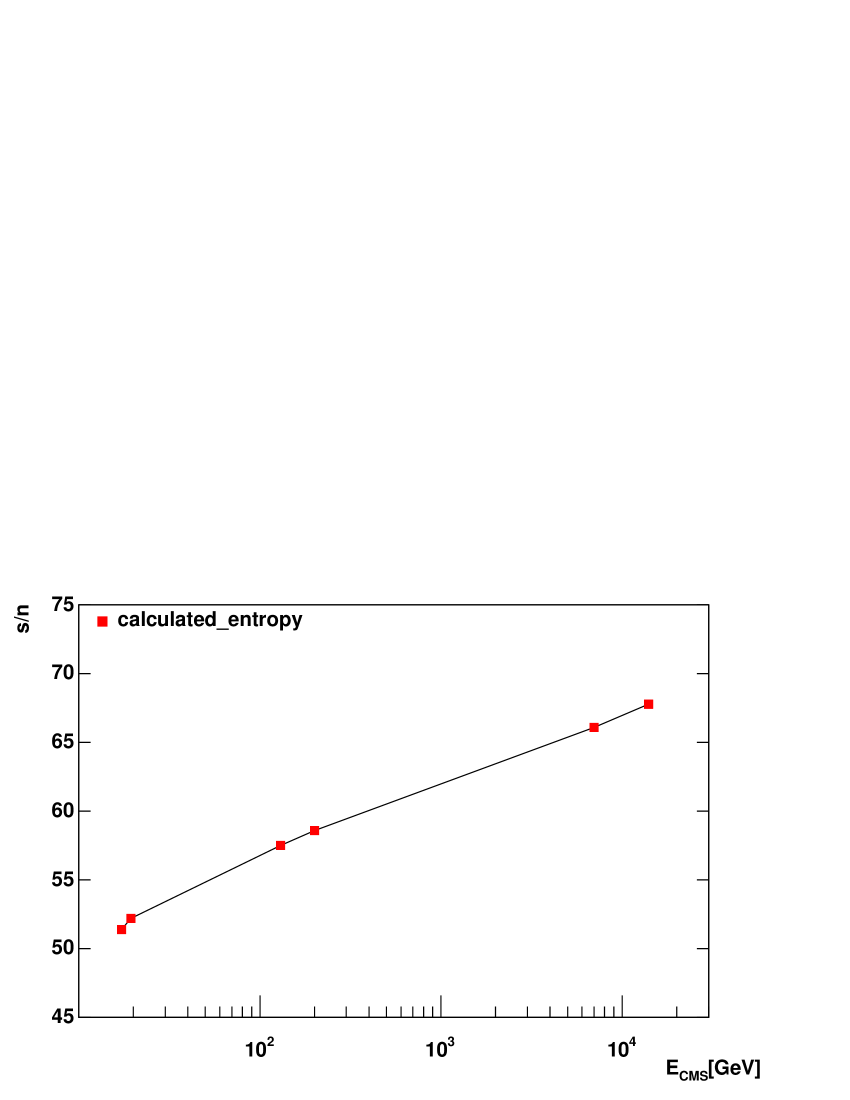
Figure 1: Calculated specific entropies at different center of mass energies. The solid line is drawn for guiding eyes.

The analysis of the curve shows that a power fit is not too bad but with a hardly interpretable power law 0.03, while a logarithmic fit S/N $\approx$ 45.31 + 2.38ln($E_{CM}$ [GeV]) is even better. The logarithmic behaviour is not surprising in an ultrarelativistic regime without energy scale.

We cannot determine the error of the calculation, but we can give mean $\chi^{2}$ deviations from the logarithmic curve. However, doing this one can see that the main deviation would come from the two SPS data points; obviously below 20 GeV we are not in the true ultrarelativistic regime. Removing these points the fit is much better, resulting in S/N $\approx$ 47.019 + 2.168 ln($E_{CM}$ [GeV]), with a $\chi^{2}$ error $\delta$(S/N) = 0.14. The error is quite low, and we will use it from 200 GeV onward. So, for the relevant energies the specific entropies are given in Table 1. The dynamic calculations give S/N=66.1 for 7000 GeV and 67.8 for 14000 GeV.

ECM [GeV]	S/N
17.3	51.4
19.4	52.2
130	57.5
200	58.6
2760	64.2
5520	65.7

Table 1: Specific entropies at various energies of center of mass.

The entropies are in the expected range. Indeed, Letessier, Rafelski & Tounsi read out almost these values from yields and energy distributions cca. 15 years ago. At $E_{beam}$ / A = 200 GeV, which is the second energy of the Table, $\sqrt{s}$ = 19.4 GeV. In 1993 the value was $50\pm 4$  let93 , in 1995 42 $\langle$ S/N $\langle$ 48  let95 and in 1996 35 $\langle$ S/N $\langle$ 60  let96 , any of them an excellent first guess.

5 Application of rehadronization schemes

The most direct experimental facts about QCD are the particle yields at the detectors. However, these particles are hadrons, coming from a hadronic phase after rehadronisation. Only their quark constituents keep the memory of the QGP phase. Therefore, the actual rehadronisation process seriously influences the yields, but we do not know a priori the correct rehadronisation model.

Here we use a variety of rehadronisation models simultaneously: each one would lead to a set of yields, and at the end one of them or at least a combination of them might be satisfactorily near to measured yields at lower energies. Then we may take this model or the combination or an extrapolation. This decision will be done in the next Section; now let us see the models used here. Calculations in models 1-10 were made a few times; of course, in contexts of much lower energies luk91 ; zim93 ; arv91 ; kfki93 ; luk96 . We consider here 10 rehadronisation models (+1 without QGP) from amongst the virtual infinity of them.

Models 1-8 assume a QG plasma at maximal compression; in the QG plasma there is complete thermal, chemical and mechanical equilibrium (processes are rapid enough). Then an expansion starts and somewhere the matter reaches the phase boundary. As a matter of simplification the phase boundary is fixed on the p-T plane, and for the actual choice see koc86 . Then rehadronisation starts, but the growing HM droplets remain in equilibrium with the QG environment (no supercooling &c.). The process goes until the last remnants of QGP vanish: then we detect the hadrons.

Even this scenario means an infinity of models, of which here we take 8, as follows. We have 3 properties of the models, and $2^{3}=8$.

1) Gluon fragmentation may occur during rehadronisation: we may neglect it (0) or may calculate it as 15% $s\overline{s}$ and 85% $q\overline{q}$. For the suggestion of this particular ratio see koc86 ; for most probable strength see zim93 ; kfki93 ; koc86 .

2) The probability of hadronic combinations may come from the quark numbers by simple combinatorics (0) or they may contain an extra factor $\sim e^{-F/T}$ (1), where F is the free energy. This latter idea is obtained from the numbers of final state microstates $\sim e^{S}$ kam86 , and for technical reasons here we will approximate F by the hadronic rest mass $m$.

3) The hadronic phase may have a compressibility of $240MeV/fm^{3}$ (1) or not (0).

The 3 numbers are regarded digital, and then add 1: so they are indeed Models 1-8. Model 9 is the absence of QGP phase at all, for simplicity’s sake with complete thermal, chemical and mechanical equilibrium throughout the whole collision, and Model 10 is a sequential fission one arv91 . A comparison of the results of Models 1-10 was given in holba up to SPS energies. We will add Model 11 in due course. All of these hadronisation models end in stables. Models ending in resonances are not considered here, because very various such models would be possible. We will later discuss the consequances of this approximation.

12 hadrons are included into the scheme, with the assumed QG precursors, as indicated:

$$N=qqq$$

$$Y(\equiv\Lambda\,\&\,\Sigma)=qqs$$

$$\Xi=qss$$

$$\Omega=sss$$

$$+antibaryons+$$

$$\pi=q\overline{q}$$

$$K=q\overline{s}$$

$$\overline{K}=s\overline{q}$$

$$\eta=s\overline{s}$$ (20)

for a while without distinguishing $u$ and $d$. All of these are ”stables”, i.e., they do not decay in strong interaction. Obviously in the initial state there is a slight $d$ excess, which may cause a bias (see next Section), but not too much, and the last mesonic representation is highly debatable but $\eta$ will not in fact be used explicitly.

Then we get unique predictions for the 12 yields if the model and the specific entropy are fixed. To demonstrate the model and specific entropy dependences, consider the ratio $\Xi/n$, for the Models 1-10 between S/N = 5 and 95 and separately between 0 and 10 on Fig. 2 and Fig. 3, respectively.

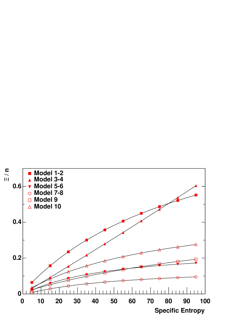
Figure 2: $\Xi/n$ ratios of model predictions above S/N=5. The solid lines are drawn for guiding eyes.

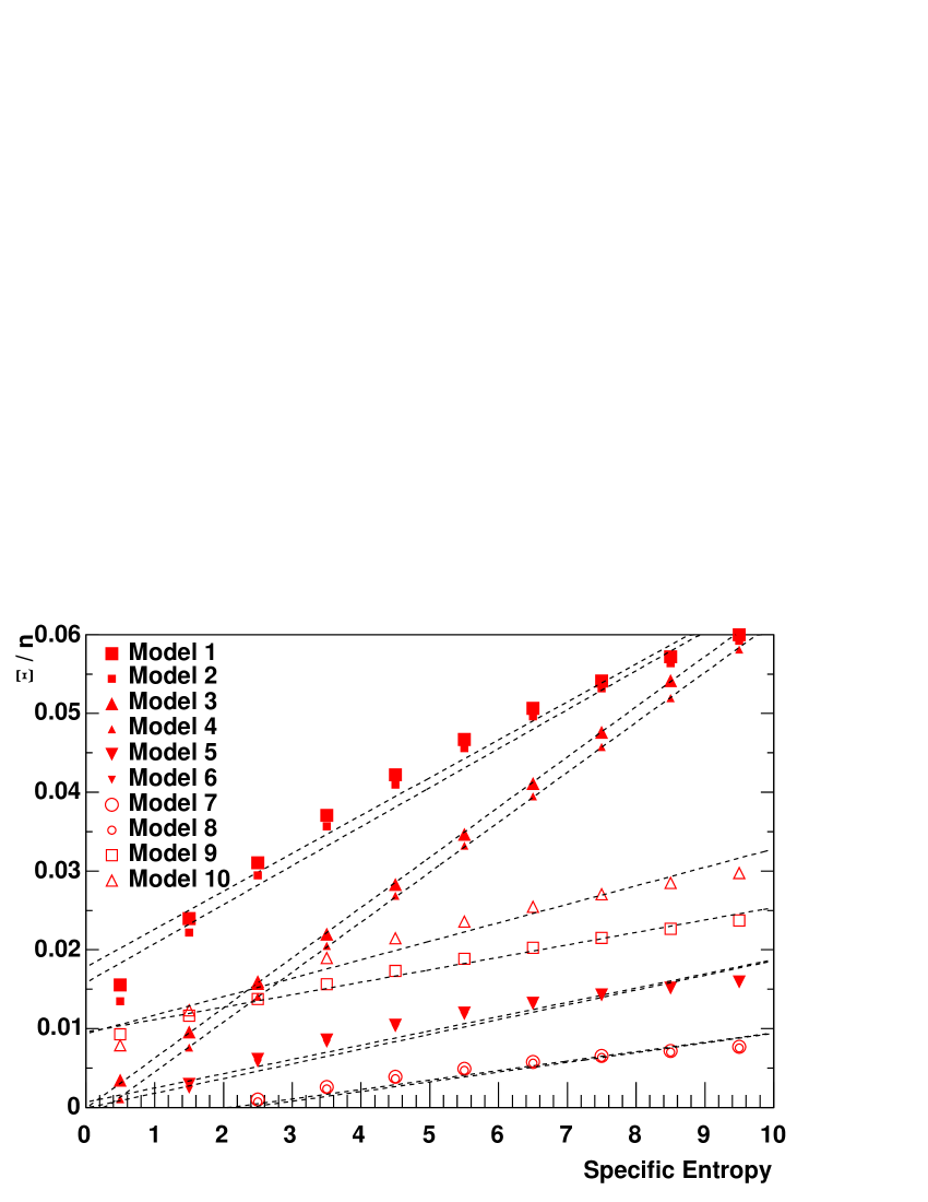
Figure 3: $\Xi/n$ ratios of model predictions between S/N=0 and 10. The solid lines are drawn for guiding eyes.

As it can be seen, for Models 1-8 there are 8 different predictions at low S/N’s, but model pairs practically coincide for S/N$>$20. So henceforth, it will be superfluous at RHIC and LHC energies to refer separately to Models 2,4,6 & 8.

Of course, very probably none of the rehadronisation models will be satisfactory because i) the rehadronisation processes do not clearly separate; and ii) some of the present models have fixed parameters which are not necessarily the true ones. Problem i) is seldom formulated explicitely, although it is serious. As an example, it is quite possible that in rehadronisation the result is not $p=uud$ but $\Delta^{+}=uud$ with parallel spins. Then $\Delta^{+}$ decays in the hadronic phase giving extra mesons, mainly pions. None of the the 11 rehadronisation models include resonances, for obvious difficulties. One of them is that very probably some $uud$ triads would correct the spin positions still in quark phase, while some $\Delta^{+}$s are formed and then decay in the hadronic phase; and we do not know, how much. (There is some indication for such decays and extra $\pi$’s at 200 AGeV RHIC as it will be seen in Section 5) We think only $\pi$ numbers will be sensitive on this. As for to overcome the second problem we can try with linear combinations of models with weights fitted to the observed yields. However, at 200 GeV the available yield ratios are limited. So we give here the method only for 3 models selected in the same time. Let the models be denoted by f, g and h, respectively; the index $i$ denotes the actual ratio. Then the actual yields are given by the combinations

$$R_{i}=a(E)f_{i}+b(E)g_{i}+(1-a-b)h_{i}+\sigma_{i}$$ (21)

where the $\sigma_{i}$’s are the errors of the combined model, to be minimized in average. This means that

$$(N-2)\sigma^{2}\equiv\Sigma_{i=1}^{N}\sigma_{i}^{2}=min.$$ (22)

Hence

$$a\Sigma_{i=1}^{N}(f_{i}-h_{i})^{2}+b\Sigma_{i=1}^{N}(f_{i}-h_{i})(g_{i}-h_{i})$$

$$=\Sigma_{i=1}^{N}(R_{i}-h_{i})(f_{i}-h_{i})$$

$$a\Sigma_{i=1}^{N}(f_{i}-h_{i})(g_{i}-h_{i})+b\Sigma_{i=1}^{N}(g_{i}-h_{i})^{2}$$

$$=\Sigma_{i=1}^{N}(R_{i}-h_{i})(g_{i}-h_{i})$$ (23)

Hence we get the best weights, and substitute them back Eq. (23) gives the average $\sigma^{2}$.

Model	158 GeV	200 GeV	130 GeV	200 GeV
	SPS	SPS	RHIC	RHIC
1 & 2	0.394	0.759	0.012	0.0503
3 & 4	1.326	2.819	0.009	0.0306
5 & 6	0.120	0.141	0.005	0.0330
7 & 8	0.165	0.283	0.005	0.0308
9	0.020	0.028	0.072	0.0950
10	0.084	0.176	0.054	0.1288

Table 2: The average predictive squared errors of the individual models.

Now we are going to compare the measured particle ratios at 158 & 200 GeV fixed target (SPS) and 130 & 200 GeV storage ring (RHIC) experiments to the predictions of the rehadronisation models 1-8, 10 plus Model 9 without QGP to find the best one or the best combination. We took the ratios from let96 ; let93 ; let95 ; let97 ; let972 ; red02 ; red022 ; tom03 ; bic04 ; let973 ; bar90 ; when we found more than one ratio but still near to each other, at a few $\sigma$, we averaged with least squares. (When they were too different we discarded one of them.) We tried to use low impact factor collisions, as far as possible. Later Table 7 will give the ratios we used in the analysis. The deviation $\sigma$ is the quantity in Eq. (22): the average ”error” of the rehadronisation model. It is dimensionless. Table 2 gives the average squared errors for individual models. However, note that if a single model is evaluated the divisor changes from N-2 to N-1.

158 GeV fixed target means 17.3 GeV in storage ring situation, at least for symmetric situations. For 200 GeV the equivalent energy is 19.4 GeV. As shown by Fig. 2 at the entropies relevant now the first 8 models give only 4 different results up to 3 digits.

The picture is clear enough: at the two lowermost energies the best predictions are given by Model 9, so a model with no QGP at all. Even Model 10, a sequential fission, is much worse. The higher error at the higher energy probably comes simply from the fact that we used less ratios there; still Model 9 wins clearly. So it seems that at those energies no well developed QGP was formed. This seems to be conform with the opinion of Ref. let96 and let973 from 1996-7 even if in the previous years still the hopes were high for 19.4 GeV, and even if Ref. let99 in 1999 still was optimistic. Just oppositely, for 130 & 200 GeVs Ref. let06 expects QGP in 2006, and indeed at this energies QGP models win. At 130 GeV the best models are 5 through 8; at 200 GeV even 3 & 4 are as good, but at the highest energy we could use only 5 ratios. So we are giving greater weight to the 130 GeV errors; but clearly we have to try with the linear combinations, as well.

There is no doubt at the two lower energies. The three-component combinations of smaller $\sigma_{i}^{2}$ always contain Models 9 or 10; if both then the weight of 10 is either smaller or even negative. With a dual combination of 9 & 10 the error minimum is at combinations with weight slightly above 1 for Model 9 and slightly negative for Model 10. Since weights either $\rangle$ 1 or $\langle$ 0 are aphysical, this means that in the whole 9-dimensional space of the linear combinations of Models 1-10 the physical optimum is at (or very near to) the pure Model 9.

For RHIC at 130 GeV the situation is more complicated. Models 5-6 and 7-8 give very similar small errors. Trial combinations with both 5 and 7 give various minima but always at aphysical weights. Dual combination of 5 and 7 is optimal at positive weight of 7 and negative one for 5. Finally an analysis of 5-7 combinations gives monotonous decrease in the physical domain from pure 5 to pure 7, but the whole difference is small: for Model 5 $\sigma_{i}^{2}$=0.0061, for Model 7 0.0058.

At 200 GeV the result is similar, although the overall error is higher (less ratios were used) and Model 3 is very sligthly better then Model 7. The squared average is generally high (which is the reason that we remain at Model 7 as best). We refer to this point in due course.

All the models 5-8 contain gluon fragmentation. So at least from the particle yields, it seems as if both a well-developed QGP and substantial gluon fragmentation appeared somewhere in the range between 20 and 130 GeV. It would be interesting to see yields between 20 and 130 GeV; but for now we go directly to 5520 GeV. We cannot expect Models 9 & 10 to overcome again at high entropy; our best educated guess is Model 7(-8). However, we give predictions of Model 5, as well, having been almost as good at 130 GeV. Because of the substantial presence of gluon fragmentation we give a Model 11, as well, which is Model 7 but with exaggerated gluon fragmentation, tuned up to the energetically possible limit. (In our language it is 1.36 instead of 1 for the gluon fragmentation parameter zim93 ; kfki93 .) Also, Model 11 may mimic somewhat rehadronisation into resonances (both processes resulting in extra light mesons).

Now, we are in the position to give the 5.52 TeV predictions. (This energy is valid only for Pb+Pb, being then Z=82 and for average isotopic coposition A=207. However this energy is almost constant in a wide range, e.g. in Au+Au it is 5.61 TeV, for example.) First we give Table 3 for stables defined in Eq. (20), still not distinguishing between the light quarks. Then we list 4 simplifications inherent in the calculations but easy to estimate for the errors caused, and even correct it in some cases.

Particle	Model 5	Model 7	Model 9	Model 11	Model 7	Mass
					(with S/N=75)	(MeV)
N	528.79	475.95	389.19	585.18	512.60	939
$\overline{N}$	326.50	301.58	152.70	365.80	350.83	939
Y	610.63	711.38	261.25	658.50	801.15	1174
$\overline{Y}$	412.91	479.61	113.76	461.67	557.46	1174
$\Xi$	79.09	38.49	59.65	26.79	44.11	1318
$\overline{\Xi}$	64.00	30.98	32.14	22.33	35.94	1318
$\Omega$	19.79	1.01	8.03	0.35	1.17	1672
$\overline{\Omega}$	19.79	1.01	5.53	0.35	1.17	1672
$\pi$	3755.23	3686.70	1775.05	4104.40	4212.90	138
K	1285.38	1388.59	965.63	1273.83	1579.55	496
$\overline{K}$	1057.50	1141.80	757.30	1068.06	1319.53	496
$\eta$	162.89	125.60	358.21	96.23	144.64	549

Table 3: The quantities of Point 4 at 5.52 TeV. Y stands for ($\Lambda,\Sigma$). The bold column is our favoured prediction.

Point 1. Slight Simplification: Insensivity on Charge and its Consequences

So far, we have not distinguished between the 2 light quarks. Therefore, N($p$)=N($n$) &c. This is definitely not true for the initial state with heavy nuclei, although it is still not an absurd approximation. The final results can somewhat be corrected according to the u/d ratio of the initial condition; but then the ratios should be calculated individually for different beams. For Pb+Pb N($u$)/N($d$)=0.87. Here we are going to make the correction.

In the charge insensitive approximation:

$$\textnormal{If}\,\,N(u)=N(d),\textnormal{then}$$

$$N(p)=N(n)$$

$$N(\Sigma^{+})=N(\Sigma^{-})=N(\Sigma^{0})=N(\Lambda)/2$$

$$N(\Xi^{0})=N(\Xi^{-})$$

and similarly for antibaryons,

$$N(\pi^{+})=N(\pi^{-})=N(\pi^{0})/2$$

$$N(K^{0})=N(K^{-})$$

and similarly for the antiparticles. (24)

(For the Y’s see App. C.)

Now, consider a well-developed QGP. Really, N($d$) $>$ N($u$). However, the asymmetry is smaller then in the initial state, because the processes creating quarks & antiquarks are charge symmetric. At the state just before the rehadronisation

$$N(d)+N(u)=1242+N(\overline{d})+N(\overline{u})$$

$$N(s)=N(\overline{s})$$ (25)

(The second formula is invalid for Model 10, and there are no quarks at all for Model 9.)

All antiquarks have been produced in charge-symmetric processes and all quarks above the initial 1242 ones, as well. Since the rehadronisation uses the same pool for any hadron, the final result is (with $R\equiv d/u$) cca. as follows. Left hand sides are the charge asymmetric yields, right hand sides are the quantities in Eq. (20).

$$p=N/(R+1),\,\,\,\overline{p}=\overline{N}/2$$

$$n=N*R/(R+1),\,\,\,\overline{n}=\overline{N}/2$$

$$\Lambda=Y*/2,\,\,\,\overline{\Lambda}=\overline{Y}/2$$

$$\Sigma^{-}=Y*R^{2}/2(R+1)^{2},\,\,\,\overline{\Sigma^{-}}=\overline{Y}/8$$

$$\Sigma^{0}=Y*R/(R+1)^{2},\,\,\,\overline{\Sigma^{0}}=\overline{Y}/4$$

$$\Sigma^{+}=Y*1/2(R+1)^{2},\,\,\,\overline{\Sigma^{+}}=\overline{Y}/8$$

$$\Xi^{0}=X*1/(R+1),\,\,\,\overline{\Xi^{0}}=\overline{X}/2$$

$$\Xi^{-}=X*R/(R+1),\,\,\,\overline{\Xi^{-}}=\overline{X}/2$$

$$\Omega^{-}=\Omega,\,\,\,\overline{\Omega^{-}}=\overline{\Omega}$$

$$\pi^{+}=\pi*(1/2)/(R+1),\,\,\,\pi^{0}=\pi/2,\,\,\,\pi^{-}$$

$$=\pi*(1/2)*R/(R+1)$$

$$K^{+}=K*1/(R+1),\,\,\,\overline{K^{+}}=\overline{K}/2$$

$$K^{0}=K*R/(R+1),\,\,\,\overline{K^{0}}=\overline{K}/2$$

$$\eta=\eta$$ (26)

For colliding nuclei others than Pb the charge-symmetric Table 3 scales with $N_{B}$, the initial $u+d=3N_{B}$, and R can be calculated from the initial u/d and from the rescaled Table 3. For Au+Au N($u$)/N($d$) = 0.88.

Point 2. A Minor Neglection in the ($\Sigma,\Lambda$) Segment

There is a slight difference between the $\Sigma$ and $\Lambda$ masses. This here will be ignored (as it will be seen, $\Sigma^{0}$ is not really observable, anyway). There is an even slighter difference amongst the $\Xi$ masses, also ignored. The reason of the mass differences is among $\Sigma$s and between $\Xi$’s that the quarks are the final components. So minimal $\Sigma$ energy is in uus combination. These differences are a few MeV’s. The mass difference between $\Lambda$ and $\Sigma^{0}$ is, however, 77 MeV. While this may still be not too serious, the real problem is that both have uds composition the relative spin positions differ. Therefore, in the ($\Lambda,\Sigma$) sector the resolution depends in somewhat arbitrary assumptions until resonances will be included. Our present assumption is discussed in Appendix D; it gives the numbers in Eq. (26) and this problem will also appear in next Section.

Point 3. The Stables

Our model includes the ”stable hadrons” of the particle physicist convention, that is those which would be stable were the s quark stable (no weak interaction). These ”stables” are:

$$n,p,\Sigma^{+},\Sigma^{0},\Sigma^{-},\Lambda,\Xi^{0},\Xi^{-},\Omega^{-}$$

the respective antihyperons, and the mesons

$$\pi^{+},\pi^{0},\pi^{-},K^{-},K^{0}_{L},K^{0}_{S},K^{+},\eta.$$ (27)

They do not decay on $10^{-23}$s scale. Without distinguishing between $u$ an $d$ (charge insensitive case) there were 12 stables as in Eq. (20); distinguishing them there will be 26 ones as in Eq. (26). However, really $\eta$ is rather obscure and it contains both $q\overline{q}$ and $s\overline{s}$. Now, observe that $\Sigma^{0}$, $\pi^{0}$ and $\eta$ are not detected. (They are ”stables”, but they do not reach the detectors). The lifetimes are long enough to survive breakup but not long enough to directly detect them. So it is only of secondary importance what is the exact quark content of $\pi^{0}$ & $\eta$. (Really, in the $O^{-}$ nonett two heavy and not too familiar measons, $\eta$ and $\eta$’, are represented by our symbolic $\eta$.) Here we regard them as the lighter composed of a light quark pair and the heavier of a strange pair. In addition obviously, Models 1-8 contain a very important neglection, mentioned already briefly. Namely, some hadrons probably will be first resonances not stables. But both rehadronisation and resonance decay are in $10^{-23}$s characteristic time, so some resonances decay in the hadronic matter, giving extra light mesons, mostly pions. This process is not included in the models, and it would be rather difficult to do it. Here, we only declare that the numbers are very probably underestimated, therefore, in all the models.

Also, there is the well known $K^{0}$ problem. For all this, see the next Point 4.

Point 4. The Observables

For handling $\Sigma^{0}$, $\pi^{0}$ & $\eta$ observe that neglecting leptons & photons $\Sigma^{0}$ decays solely to $\Lambda$, $\pi^{0}$ decays solely to nothing, and $\eta$ gives a $\pi^{0}$ (which then decays into nothing) or either nothing else or a $\pi^{+}\pi^{-}$ pair. Since $\Sigma^{0}$, $\pi^{0}$ & $\eta$ decay before the detectors, in them we get:

$$\Sigma^{0}\rightarrow 0$$

$$\Lambda\rightarrow\Sigma^{0}+\Lambda$$

$$\pi^{0}\rightarrow 0$$

$$\eta\rightarrow 0$$

$$\pi^{+}\rightarrow\pi^{+}+0.29*\eta$$

$$\pi^{-}\rightarrow\pi^{-}+0.29*\eta$$ (28)

where $\rightarrow$ does not mean any temporal sequence but a calculation of detectables. For $K^{0}$’s the detectable components are $K^{0}_{L}$ and $K^{0}_{S}$, for which

$$K^{0}_{L}=K^{0}_{S}=(K^{0}+\overline{K^{0}})/2$$ (29)

This way we still have, say, $\Sigma^{0}$ if it can be reconstructed, which is sometimes claimed.

6 Discussion

Earlier we have told that at lower energies (158 & 200 GeV/nucleon fixed target) the model best for reproducing the yield ratios amongst the 11 ones included in the present survey was Model 9, the only one without QGP phase at all. This is a signal that at these energies pure quark phase is still absent. However, at 130 & 200 GeV per nucleon storage ring energies the two best models are 5 (”100”) and 7 (”110”). Model 7 is marginally better, and linear combination does not improve the performance: at 200 GeV the situation is not clear but Model 7 is better then Model 5. Note that individual yields may differ between Models 5 & 7; only they are near to each other in overall performance.

Since this fact indicates well-developed QGP already at 200 GeV, we do not expect anything else at 5.52 TeV. Therefore, our favourite prediction is Model 7; but we do not deny a slight chance from Model 5. As for Model 9, the one without QGP, we give its yields only for comparison. Model 11 is Model 7 but with the maximal possible gluon fragmentation. Finally, we give also the predictions of Model 7 for S/N = 75 (instead of the expected 65.7); the reason will come. The final results are in Table 6; then you can calculate any ratios of the observables taking into account Eqs. (28, 29). As for the error of the prediction, in theory the $\chi^{2}$ test at 200 GeV suggests  $\pm 0.02$ in ratios, but the $\sigma$’s in Table 2 show that there are serious biases, too.

Of course most biases/systematic errors are unknown, but we can estimate 2 of them.

First, as told in Point 1 of Section 5, the simplified model overestimates the number of quarks $u$. Because of heavy nuclei in the beam the true $u/d$ ratio is $\approx$ 0.87 ($Pb+Pb$). Now, all in the ratios $\Sigma^{+}/p$, $\Omega^{-}/\Xi^{-}$ and $\pi^{-}/K^{-}$ the ratio N($s$)/N($d$) appears, and N($d$) is in reality greater than in the model by cca. 6 % relative. However, note that this distortion is less in Model 7 where the gluon fragmentation somewhat dilute the $d$ surplus, and even less in Model 11. And in Table 6 we will give the charge-sensitive yields according to Eq. (26).

The second type of error may come from the thermodynamic nature of the models; in them particle number conservations are not explicit. But the final particle numbers can check the accuracies. Table 4 summarizes some results of Table 3.

Total $N^{o}$	Initial	Model 5	Model 7	Model 9	Model 11
Particle	-	8322.50	8382.70	4878.44	8653.47
Strangeness	0	0.02	0.00	1.68	-0.01
Baryon	414	415.10	413.65	413.99	420.68

Table 4: Conservation checks for Pb+Pb collisions with 5.52 TeV/nucleon-pair.

We can see that Models 7 & 9 are excellently consistent with the conservation laws, and the relative errors are low even for Models 5 & 11, because the baryon number & strangeness conservations should be maintained in the presence of lots of particles with negative quantum numbers. If we relate the above errors to the averages of numbers of particles with + & - quantum numbers, then at the worst cases the relative error is 0.1% for strangeness and 0.7% for baryon number.

Observe the tremendous particle production in the collisions. Just after breakup there are at least an order of magnitude more particles present than in the initial condition. As for the differences between the total yields of the models we see some 1% difference between Models 5 & 7, hardly more between 7 & 11 and the only serious difference is Model 9 without QGP phase.

Charge conservation will be checked after the charge-asymmetric Table 6.

Table 5 gives us the data for estimating the efficiency turning the beam energies into ”something”. At the initial condition there are 414 nucleons, each with 2760 GeV kinetic energy. Just after rehadronisation/breakup some of the kinetic energy has turned into rest mass, some into internal energy in thermodynamic sense, and some energy has gone away in the beams. Calculating with a 160 MeV temperature at rehadronisation as approximately got in Models 1-8 & 11, the numbers are as follows: where $E_{transf}$ does include the rest masses, but not the ones present in the beginning. At the initial condition $E_{transf}$ was 0, and $M_{tot}$/414 was 0.94 GeV.

Model #	$E_{tot}/414$ [GeV]	$M_{tot}/414$ [GeV]	$E_{transf}/414$ [GeV]
5	2760	9.73	13.62
7	2760	9.80	13.72
9	2760	5.77	7.66
11	2760	9.78	13.86

Table 5: Conversion of initial kinetic energy $E_{tot}$ into energy transferred to new particles.

So we can see that the efficiency of conversion is predicted to be $(3~{}-~{}5)*10^{-3}$ at 5.52 TeV. The reason is of course the forward-peaked differential cross section. (As told earlier if rehadronisation goes through resonances, not included in the models, then the resonances yield extra light mesons. This, of course increases the kinetic energy transferred to masses. However, the effect is not big. Doubling the number of pions the last column of Table 5 goes up with cca. 1.5)

At last, we are going to investigate the unavoidable consequences of the present lack of observations at energies between Tevatron and LHC. In Section 4 we evaluated the expected LHC specific entropy and we got 65.7. However, the experimental differential cross sections are not yet measured above Tevatron momenta; we have used extrapolations islam assuming that nothing new happens there. This is probably so; but if we cross the energy range of ”something new” between Tevatron and LHC energies, then in first approximation a ”reasonance peak” is expected, so increasing the cross section and so the S/N. This ”something new” might be anything (e.g. crossing the supersymmetry energy scale) and we have no preferred candidate, at all. It will not be necessary either; we can simply perform calculations with our best, Model 7, with S/N = 75 (some 10% increase) for the observables according to Point 5.

Now, we make the charge-sensitive evolution of yields for Pb+Pb. Accepting the charge-insensitive yields of Table 3, we operate as told earlier for u’s and d’s in Point 1, so finally:

$$N(u)=578+(1/2)[N(q)-1242]$$

$$N(d)=664+(1/2)[N(q)-1242]$$

$$N(s)=N(\overline{s})$$

$$N(\overline{u})=N(\overline{d})=(1/2)[N(q)-1242]$$ (30)

with this we get Table 6, with stables, with our definite prediction in column 3, Model 7, S/N=65.7; if any of the other columns will have been proven superior, one can at least guess hence the reason. For the detected ones one can use Eqs. (28, 29). We have chosen this way, because indirect methods may reconstruct at least $\Sigma^{0}$ and $\pi^{0}$. For comparision, the last column gives figures of Model 7 for 200AGeV at RHIC. At this point we can check charge conservation. Interestingly, charge conservation depends on the handling of the ($\lambda,\Sigma$) sector. We tried two different decompositions of $Y$’s into $\lambda$ and $\Sigma$ which will be discussed in Appendix D. Exact charge conservation would mean Z=164; at the first choise $Z\approx 174$ for all the models, in the second one $Z\approx 172$. So we used the second for yields, but our calculations seem to indicate that further supression of $\Sigma$s do not help in charge conservation. Note, that our rehadronisation models are thermodynamic, charge asymmetric states are not of minimal energy. Therefore, thermodynamic models have the tendency to violate charge conservation. Anyway, the net error 5% correspond to error/all charged $\approx$ 0.2%, in the order of the errors for strangeness conservation.

Particle	Model 5	Model 7	Model 9	Model 11	Model 7	Model 7
					(with S/N=75)	(200 GeV RHIC)
p	261.53	235.41	190.87	289.62	253.85	221.30
$\overline{p}$	163.25	150.79	76.35	182.90	175.42	131.99
n	267.26	240.54	198.32	295.56	258.76	226.66
$\overline{n}$	163.25	150.79	76.35	182.90	175.42	131.99
$\Sigma^{+}$	74.68	87.01	31.42	80.65	98.23	78.45
$\overline{\Sigma^{+}}$	51.61	59.95	14.22	57.71	69.68	52.52
$\Sigma^{0}$	152.64	177.82	65.29	164.61	200.27	160.69
$\overline{\Sigma^{0}}$	103.23	119.90	28.44	115.42	139.37	105.04
$\Sigma^{-}$	77.99	90.85	33.92	83.99	102.07	82.29
$\overline{\Sigma^{-}}$	51.61	59.95	14.22	57.71	69.68	52.52
$\Lambda$	457.95	533.51	195.91	493.86	600.84	482.12
$\overline{\Lambda}$	309.68	359.71	85.32	346.25	418.10	315.13
$\Xi^{0}$	39.12	19.04	29.25	13.26	21.84	16.90
$\overline{\Xi^{0}}$	32.00	15.49	16.07	11.16	17.97	13.60
$\Xi^{-}$	39.97	19.45	30.40	13.54	22.26	17.30
$\overline{\Xi^{-}}$	32.00	15.49	16.07	11.16	17.97	13.60
$\Omega^{-}$	19.79	1.01	8.03	0.35	1.17	0.89
$\overline{\Omega^{-}}$	19.79	1.01	5.53	0.35	1.17	0.89
$\pi^{+}$	928.62	911.72	435.26	1015.69	1043.13	811.42
$\pi^{0}$	1877.62	1843.35	887.53	2052.50	2106.45	1642.49
$\pi^{-}$	948.99	931.63	452.26	1036.51	1063.32	831.07
$K^{+}$	635.72	686.80	473.57	630.45	782.21	613.97
$K^{-}$	528.75	570.90	378.65	534.03	659.77	503.06
$K^{0}_{L}$	589.21	636.35	435.36	588.70	728.55	565.94
$K^{0}_{S}$	589.21	636.35	435.36	588.70	728.55	565.94
$\eta$	162.89	125.6	358.21	86.23	144.64	111.06

Table 6: The predicted hadronic observables in a central $Pb+Pb$ collision at 5.52 TeV/nucleon-pair CM energy.

In Table 7 we give all the abundance ratios which we used in Section 5; the data will show the qualities of the models in the last column. The experiments and the references are identified, too. We have ignored individual data that seem to be direct contradictions to data referred here. In case of 158 AGeV SPS we have not used $K^{+}/\pi^{+}$ and in case of 130 AGeV RHIC we have not used $\Omega/\pi^{-}$, $K^{-}/\pi^{-}$, $\overline{p}/\pi^{-}$ because we were not convinced that the pion background does not adulterate the ratios. (Again, hadronisation into resonances being neglected) In contrast, such ratios were kept for 200 AGeV RHIC because of the shortage of ratios at this energy. If one does not like such ratios, one can use a derived experimental ratio $K^{-}/\overline{p}$ instead of the last 2 rows given in the brackets. The predictions of the models with least average errors are given, too: Model 9 for the first 2 energies and Model 7 for RHIC energies.

Energy/nucl.	Ratio	Experiment	Reference	Measurement	Model 9
158 GeV SPS	$\Xi^{0}/\Lambda$	WA97	let972	$0.14\pm 0.02$	$0.14\pm 0.13$
	$\overline{\Xi^{0}}/\overline{\Lambda}$	WA97	let972	$0.26\pm 0.05$	$0.19\pm 0.13$
	$\Omega/\Xi^{0}$	WA97	let972	$0.19\pm 0.04$	$0.27\pm 0.13$
	$\overline{\Omega}/\overline{\Xi^{0}}$	WA97	let972	$0.30\pm 0.09$	$0.35\pm 0.13$
	$\overline{\Lambda}/\Lambda$	WA97, NA49	let972	$0.145\pm 0.024$	$0.38\pm 0.13$
	$\overline{\Xi^{-}}/\Xi^{-}$	WA97	let972	$0.27\pm 0.05$	$0.49\pm 0.13$
	$\overline{\Omega}/\Omega$	WA97	let972	$0.42\pm 0.12$	$0.66\pm 0.13$
	$(\Xi^{-}+\overline{\Xi^{-}})/(\Lambda+\overline{\Lambda})$	NA49	let972	$0.13\pm 0.03$	$0.16\pm 0.13$
	$\overline{\Lambda}/\overline{p}$	NA49	let06	$1.05\pm 0.16$	$1.12\pm 0.13$
	$K^{-}/K^{+}$	NA49	red02	$0.59\pm 0.05$	$0.77\pm 0.13$
200 GeV SPS	$\overline{\Lambda}/\overline{p}$	NA35	let97	$0.80\pm 0.25$	$1.12\pm 0.14$
	$\Xi^{-}/\Lambda$	WA85	let96	$0.19\pm 0.01$	$0.15\pm 0.14$
	$\overline{\Xi^{-}}/\overline{\Lambda}$	WA85	let96 ,let97	$0.21\pm 0.02$	$0.19\pm 0.14$
	$(\Omega+\overline{\Omega})/(\Xi^{-}+\overline{\Xi^{-}})$	NA35	let97	$0.80\pm 0.4$	$0.28\pm 0.14$
	$\overline{\Lambda}/\Lambda$	NA35	bar90	$0.18\pm 0.06$	$0.38\pm 0.14$
					Model 7
130 GeV RHIC	$\overline{p}/p$	STAR	red02 , red022	$0.64\pm 0.05$	$0.59\pm 0.06$
	$\overline{\Omega}/\Omega$	STAR	tom03	$1.00\pm 0.2$	$1.00\pm 0.06$
	$\overline{\Lambda}/\Lambda$	STAR	red02 , red022	$0.77\pm 0.05$	$0.65\pm 0.06$
	$\overline{\Xi^{-}}/\Xi^{-}$	STAR	red02 , red022	$0.81\pm 0.05$	$0.78\pm 0.06$
	$\pi^{-}/\pi^{+}$	PHOBOS	red022	$0.95\pm 0.06$	$1.02\pm 0.06$
	$K^{-}/K^{+}$	STAR	red022	$0.90\pm 0.05$	$0.82\pm 0.06$
200 GeV RHIC	$\overline{p}/p$	PHOBOS, PHENIX	tom03 , bic04	$0.84\pm 0.04$	$0.60\pm 0.16$
		STAR, BRAHMS
	$K^{-}/K^{+}$	PHOBOS, PHENIX	tom03 , bic04	$0.98\pm 0.04$	$0.82\pm 0.16$
		BRAHMS
	$\pi^{-}/\pi^{+}$	PHOBOS	bic04	$1.02\pm 0.02$	$1.02\pm 0.16$
	$K^{-}/\pi^{-}$	STAR, BRAHMS	tom03	$0.15\pm 0.02$	$0.61\pm 0.16$
	$\overline{p}/\pi^{-}$	BRAHMS	tom03	$0.08\pm 0.01$	$0.16\pm 0.16$
	($K^{-}/\overline{p}$	STAR, BRAHMS	tom03	$1.87\pm 0.34$	$3.81\pm 0.16$)

Table 7: Experimental and model particle ratios for different collision energies. The errors of the penultime column are that of the ratio measurements. The average errors of the models can be obtained from Table 2 as: 0.13 for 158 GeV SPS, 0.14 for 200 GeV SPS, 0.06 for 130 GeV RHIC, and 0.16 for 200 GeV RHIC.

Now, let us compare methodically the measured and predicted ratios. Generally, they must agree because the model errors were estimated in Eq. (22) and Table 2 from the differences. However, it is interesting to see the possible individual big differences which would signal shortcomings of even the best model of the original 1-10. Henceforth we study the deviations $r_{i,obs}-r_{i,mod}$ whose errors are composed from the individual measurement errors and the model error. As for the error of the difference $\Delta$, its distribution is the convolution of those of the r’s, so the second central momentum is the sum of the constituents janos , i.e.

$$\sigma^{2}=\sigma_{1}^{2}+\sigma_{2}^{2}$$ (31)

but of course we do not know the distribution, only that it is nearer to Gaussian than those of the r’s.

Using the good rehadronisation model, the observed r’s should fluctuate around the model predictions, so the set ${\Delta_{i}}$ denoting individual ratios should fluctuate around 0. Table 6 contains 26 independent ratios. Which of them 16 is not farther from 0 than 1$\sigma$. For the remaining 7 we get Table 8.

Experiment	Ratio	$\Delta$	$\sigma$	Deviation/$\sigma$	Error integral
158 GeV SPS	$\overline{\Lambda}/\Lambda$	-0.235	0.13	1.85	0.06
158 GeV SPS	$\overline{\Xi^{-}}/\Xi^{-}$	-0.22	0.14	1.57	0.12
158 GeV SPS	$\overline{\Omega}/\Omega$	-0.24	0.18	1.33	0.18
158 GeV SPS	$K^{-}/K^{+}$	-0.18	0.14	1.28	0.20
200 GeV SPS	$\overline{\Lambda}/\overline{p}$	0.32	0.29	1.10	0.27
200 GeV SPS	$(\Omega+\overline{\Omega})/(\Xi^{-}+\overline{\Xi^{-}})$	0.52	0.42	1.24	0.22
200 GeV SPS	$\overline{\Lambda}/\Lambda$	-0.20	0.15	1.33	0.18
130 GeV RHIC	$\overline{\Lambda}/\Lambda$	0.12	0.08	1.50	0.13
200 GeV RHIC	$\overline{p}/p$	0.24	0.16	1.50	0.13
200 GeV RHIC	$K^{-}/\pi^{-}$	-0.46	0.16	2.88	0.004

Table 8: 10 ratios in Table 7 whose $\sigma$’s are above 1 with one ratio whose $\sigma$’s is above 2. The difference $\Delta$ of columns 5 & 6 is within 1$\sigma$ in 16 cases.

There was really no measurement for the synthetic last bracketed ratio at 200 GeV RHIC, so that value is not analysed here. The last column is the error integral

$$1-erf(n)=\sqrt{2/\pi}\int_{n}^{\infty}\!e^{-u^{2}/2}\mathrm{d}u$$ (32)

Were the distribution of $\Delta$ Gaussian, the last column would show the probability of such a random fluctuation; it is at least an estimation for it. The position is the position within the actual group in Table 7.

Individual measurements up to 2$\sigma$ are generally not regarded as too problematic. So 9 out of the 10 ratios outside 1$\sigma$ are not necessarily signals of problems. $\chi^{2}$ tests might be advisable, but will not be done here. However, the $K^{-}/\pi^{-}$ ratio at 200 GeV RHIC is surely problematic.

Our guess is that we see consequences of enhanced pion yields, and it is probably enhanced by rehadronisation into resonances. As discussed already in Section 4, Point 2, the encounter of quarks may result in resonances instead of stables. Were the timescale of phase transition significantly longer than the resonance lifetimes, the quarks could try again. However, both timescales are $10^{-23}$ s, so the two processes do not clearly separate; some resonances may decay in the hadronic phase, giving extra mesons, mainly $\pi$’s.

We are not really manufacturing a full Model 12 including resonances; a lot of presently badly known new parameters should be used for that. But just for demonstration consider the case when the final baryon yields are unchanged, but half of them come through the corresponding member of the decuplet. (Of course, $\Omega$ is an exception, being a stable and, in the same time, a member of the decuplet.) Then 3 model predictions of the 5 200 GeV RHIC yields in Table 6 are unchanged, but 2 gives new results. For estimation take the model errors equal to that of Model 7; then we get Table 9. That is our ”Model 12”; The quotation marks are used because it not a fully elaborated model but rather an estimation.

Experiment	Ratio	$\Delta$	$\sigma$	Deviation/$\sigma$
200 GeV RHIC	$K^{-}/\pi^{-}$	-0.11	0.16	0.69
200 GeV RHIC	$\overline{p}/\pi^{-}$	0.09	0.16	0.57

Table 9: The so far problematic ratios at 200 GeV RHIC in ”Model 12”.

Both problematical ratios have got within 1$\sigma$ to 0.

So surely there are stables which resulted through resonances. Surely pion numbers will be then higher than in the present models. However, kaon numbers would be unchanged in first approximation since the decays mainly go as $X^{*}\rightarrow X\pi$. So either we should handle the resonances properly before predictions are made; or as a first step we should ignore any ratio involving pions. As a second step, the $\pi$ surplus will be between 0 and the sum of the numbers of 1/2-spin baryons + antibaryons.

The synthetic ratio $K^{-}/\overline{p}$ is still rather high from Model 7 compared to the ratios of 2 measured ratios. However, the statistics of such derived quantities need serious cautions.

We emphasize that an almost infinite number of different models can reproduce more or less the yields published so far. Our models are focused on rehadronisation, but they were not too interested about, say, collective phenomena in the QG or hadron phase. Such collective phenomena may cause quite remarkable effects, as e.g. verte can predict very enhanced $\eta$’ yields, and then $\pi$ production, via the mass of $\eta$’ meson much lower than the free mass. Such effects are actually quite importans. However, note that $\eta$’, while it is technically a stable, is rather a short lived particle with $10^{-21}$s lifetime and the situation is unfamiliar as in luk86 shown many years ago that even existing particleis may or may not form an independent thermodynamic degree of freedom. In addition, lots of formally different approches may result in similar yields, as it was shown in luk86 . At the present status of knowledge we rather want to compare as many models as possible and we are not looking for the best one.

At the end of this Section it is the proper place to note that there are very preliminary yields from the new range about $E_{CM}$ = 2.76 TeV. E.g. mulle gives 2*4 ratios for nearly central collisions, without error bars. For antiparticles the ratios are almost exactly the same as for particles, and, according to what we mentioned above, it is better to leave out the pions. Then we remain with three ratios, $K^{+}/p$, $\Xi^{-}/p$ and $\Omega/p$. Comparing these very approximate ratios with predictions of Model 7 for 0.2 & 5.52 TeVs we get Table 10.

Ratio	0.2 TeV, Model 7	2.76 TeV, prelimininary	5.52 TeV, Model 7
		measurement
$K^{+}/p$	2.8 $\pm$ 0.34	3.2	2.9 $\pm$ 0.49
$\Xi^{-}/p$	0.078 $\pm$ 0.013	0.12	0.083 $\pm$ 0.014
$\Omega/p$	0.004 $\pm$ 0.0007	0.02	0.004 $\pm$ 0.0007

Table 10:

Comparison to non-pionic preliminary ratios for 2.76 TeV in mulle . The errors of the model calculatios are based on Table 6.

While the first two ratios would be within error after the manner of Table 7, $\Omega/p$ of Model 7 is too big, by cca. a factor of 5. However, Model 5 would give a ratio even bigger by almost 8. This again would suggest something between Models 5 & 7 as it was seen in Section 5 at RHIC energies.

7 Conclusion

At the end we should answer the question of QG phase. In some sense we have done that: we predict the yields of our Model 7, with S/N=65.7, Column 3 of Table 6. Now, Model 7 contains a phase transformation into QGP, then a definite amount of gluon fragmentation, and then a rehadronisation according to some rules. So if the yield ratios will be near to those calculable from our preferred Column 3, then indeed the detected ratios confirm the transient existence of the QGP. However, the old story of too much $K^{+}$ in 1987 plos ; tann ; luk900 is a warning that even a good agreement with the predicted ratios would not be a proof. A proof would be almost impossible. Observe that, e.g., a completely hadronic explanation of ”too much” $K^{+}$ at 14.5 GeV fixed target could be ”simply” an enhanced rate of the reaction

$$p+p\rightarrow p+K^{+}+\Lambda$$ (33)

above T=150 MeV.

Namely, the existence of a QG phase is something with definite meaning only in thermodynamic context; and lan61 gives the rigorous prescription to decide if a definite thermodynamic phase is present. We cannot perform the needed operations in the later hadronic phase. In principle leptons may originate in QGP and so carry some direct information; but that is beyond the scope of the present paper.

As told earlier, our preferred prediction is Column 3 of Table 6. You can form then the actual ratios measured in the future. (Corrections for the slight $d$ to $u$ surplus at initial condition have been done in Table 6.) The other columns are partly for comparison, partly for cases when ”something unexpected happens” between TEVATRON and LHC energies.

We have seen that at RHIC energies the performance of our Model 5 was only slightly worse that of Model 7; but combination of the two models did not help, so Model 7 was chosen as the absolute best. Now, Model 5, without the selecting mechanism of hadronic final state data, results in more heavy hyperons than Model 7 (in $\Omega$ the increase is almost 20-fold), and therefore, slightly less lighter ones. It is not quite impossible that with increasing energy the combinations feel less the final state masses; not because of higher energy (entropy would not increase much) but because less time for new trials in hadron formation; but still we believe rather in Model 7. But data of mulle suggest that the model might suppress $\Omega$ too strongly, while Model 5 does not do it sufficiently.

Model 11, Model 7 with enhanced gluon fragmentation, would be observed, according to Column 5, as slight increases in lighter antihadrons and slight decreases in heavier ones. The differences are moderate, and it is questionable if the observations will be able to distinguish Models 7 & 11. Yield ratios nearer to Model 11 than to Model 7 would not automatically suggest enhanced gluon fragmentation; rehadronisation into resonances and then decay in the hadronic matter leads to a $\pi$ surplus which is also true at enhanced gluon fragmentation. On the other hand, it seems that higher S/N (last column in Table 6) would be distinguishable from resonance decay. Anyway, $K^{-}/\pi^{-}$ and $\overline{p}/\pi^{-}$, we think, again could signal resonance decays in hadronic phase if the ratios were much smaller than any columns of Table 6. ”Model 12”, as told, is not a full model but an estimation for the pion surplus from resonances. We simply assumed that during the hadronisation half of the emerging baryons were stables and the other halp resonances. The resonances decay in the hadronic phase. This ”Model” has been explained at the end of Section 6.

Column 6 shows the outputs for Model 7 at a higher S/N=75. The entropy would increase if something unexpected happens with the cross sections between TEVATRON and LHC energies. For ratios the differences between Columns 3 & 6 are slight, because all particle yields increase in Column 6. Maybe the difference would be observable in the antiparticle/particle ratios; they are higher in Column 6, but the difference is not greater than 3 %.

And finally, let us see the famous $K^{+}/\pi^{+}$ ratio which provoked discussions back to 1987 about the formation of QGP plos ; tann ; luk900 ; which lead to the ALCOR model in 1999 zim00 , and which was in early times in general expected a good QGP signal. For comparison we give $K^{-}/\pi^{-}$ in Table 11, as well.

	Year-1987	Model 5	Model 7	Model 9	Model 11	Model 7
Note	14.5 GeV fixed t.	fragmentation	favourite	hadronic	enh.fragmentation	S/N=75
$K^{+}/\pi^{+}$	0.24	0.685	0.753	1.088	0.621	0.750
$K^{-}/\pi^{-}$	$\approx$0	0.557	0.613	0.837	0.515	0.620

Table 11: $K/\pi$ ratios in Pb+Pb reactions at 5.52 TeV.

Now, the morale is clear but somewhat disturbing. At ”low energies” a $K/\pi$ ratio much higher for kaons than for antikaons had been believed to be a quark signal. But for 5.52 TeV all models give higher $K^{+}/\pi^{+}$ than $K^{-}/\pi^{-}$ ratios; and the highest ratios are given by Model 9 completely without QGP! (See also the $K/\pi$ discussion in holba )

One possible conclusion is that great care is needed when looking for signals. Another is that maybe at high energies the situation differs from those at lower ones. Both conclusions are indeed probable, even if not quite quantitative. However, there is something more, to which Table 11 is a warning.

Models 1-8 & 10-11 contain QGP, with quarks in equilibria within (probably a good assumption, reaction times being guessed short in QGP); the rehadronisation assumptions differ (and they may be not equilibrium ones). The completely hadronic Model 9 contains hadrons in equilibria.

Now, for the QGP quark to antiquark surplus is necessary because of initial condition, except for s, where $\overline{s}/s$=1 because all strange quarks were produced in QGP and strangeness is conserved.

Being $K^{+}=(u\overline{s})$ and $K^{-}=(\overline{u}s)$, the ratio $K^{+}/K^{-}>$ 1 is nontrivial from quark composition. However, note that all models with QGP feel the initial conditions, so produ ce baryon to antibaryon surplus. Then $K^{+}/K^{-}>$ 1 is a necessary consequence of conservations.

As for Model 9 without QGP it is an equilibrium model. If time were long enough, high $K/\pi$ ratios would be obtained. Now, in 1987 the time estimated seemed not enough for this, and we still believe this, because $K^{-}/\pi^{-}$ was cca. 0 tann . Namely, consider initial N+N collisions. The simplest result is 3 particles, say N, a hyperon and a kaon. Antikaon instead of kaon is impossible for 3 particles because of strangeness conservation. Therefore, reactions resulting in $K^{-}$ would have low rates anyways; although the energy barrier is much lower in QGP for $qqq\rightarrow qqqs\overline{s}$ then in HM for $NN\rightarrow NK\Lambda$, cca. 300 MeV in the first case and almost 700 MeV in the second. So $K^{-}/K^{+}<<$ 1 in 1987 in itself was not a signal either for or against liberated quarks, only against quarks in complete equilibrium; a ”too high” $K^{+}$ number suggested liberated quarks, but because of $K^{-}/K^{+}<<$ 1 is not a ”quite proper” QGP.

It seems that at RHIC energy, S/N=58 a proper QGP phase was formed. We cannot prove this being the QGP unreachable for us; but the hadronic yields prefer QGP. Then we have no reason to doubt in QGP at 5.52 TeV.

Acknowledgements

We think formal acknowledgements are unnecessary to the colleagues referred below. J. Zimányi triggered the studies and gave lots of impetus for us. H-W. Barz, T. S. Biró, L. P. Csernai, T. Csörgő, B. Jakobsson, B. Kämpfer, Gy. Kuti, P. Lévai, K. Martinás, L. Polonyi, K. Szlachányi, Gy. Wolf were not only coauthors of one of the present author in works cited here, but also they worked in producing/improving the models used here. Thanks go to Gösta Gustafson of University of Lund for valuable discussions. The authors gratefully acknowledge the support of the Hungarian OTKA grant NK 101438.

Appendix

Appendix A List of the used rehadronisation models

Here we use 12 models, that, however, are practically 8 at LHC energies. They are as follows. Models from 1 to 8 are rehadronisation model in $2^{3}$ arrangement, as a binary number + 1. The models were discussed in Ref. luk91 & luk96 . The conditions for the states of the 3 digits are as follows:

1. Final state compressibilty is involved (1) or not (0). On this digit, however, dependence is negligible at 2.76+2.76 TeV.

2. Final state hadronic masses are taken into account (1) or not (0). This influences the yields and the best model cannot be selected a priori because the rehadronisation is not an equilibrium process.

3. Gluon fragmentation takes place in QGP (1) or it does not (0). If it does, we take its parameters from Ref. koc86 .

So Models 1-8 refer to the 3 digit states ”000”-”111” according to Table 12, in summary.

Model	Gluon	Hadronic	Final state
#	fragmentation	masses	compressibility
1	0	0	0
2	0	0	1
3	0	1	0
4	0	1	1
5	1	0	0
6	1	0	1
7	1	1	0
8	1	1	1

Table 12: A group of rehadronisation models including the 3 options in columns 2-4.

Model 9 is a purely hadronic phase one, and Model 10 is a sequential fission one, see Refs. luk91 & luk96 .

Model 11 is a version of Model 7, but with gluon fragmentation enhanced to the energetically possible maximum, see Ref. zim93 & kfki93 .

Model 12 is not an entirely elaborated model, but an educated guess, when everything starts as in Model 7, but half of the resulting baryons enter the hadronic phase as resosances and the decay there, giving surplus mesons, mainly $\pi$’s.

Appendix B Transformation to partially specific variables

Eq. (12-14) guarantee that we can calculate functions from $\hat{s}$. Now, let us use $\hat{s}$.

As told Uneq. (5) must hold, for any timelike $u^{i}$ field. In $\hat{s}_{;r}$ the derivatives $n_{,r}u^{r}$ and $e_{,r}u^{r}$ can be substituted from Eqs. (3,4) and then we get

$$\hat{s},_{t}Dt+(\hat{s}-n\hat{s},_{n}-e\hat{s},_{e}-k\hat{s},_{e})u^{r};_{r}+t^{r}(z,_{r}-\hat{s},_{e}\beta,_{r})$$

$$+t^{r};_{r}(z-\hat{s},_{e}\beta)-\hat{s},_{e}\beta t^{r}u^{s}u^{r;s}-\hat{s},_{e}(\gamma-k/t^{2})t^{r}t^{s}u_{r;s}$$

$$\geq 0$$

$$D\equiv u^{s}\partial_{s}$$ (B.34)

identically i.e. for any u; and several terms apppear with quite various u-dependences. Collecting the terms with the same u-dependences, Uneq. (5) is guaranteed only if the terms of different u-dependences satisfy equations independently. That is set in Eq. 15).

Appendix C Evaluation of $\lambda$ of ultrarelativistic collisions

This Appendix is necessary to avoid inconsistencies in the main text. Namely, in this paper t stands for 3 quite different quantities: time, the specific extra extensive and one invariant familiar in 2-particle collisions. Similarly, s means both entropy density and another invariant, while $u$ is both the velocity vector and the third invariant. So we have separated the part most confusing and here we try to be careful and explicit in the formulation.

Consider an elastic two-body collision where the incoming two particles have the original momenta of the beams. By appropriate choice of the coordinate system and by momentum conservation we always can write:

$$u_{1/2}^{i}=\{(1+v^{2})^{1/2},\pm v,0,0\}$$

$$u_{3/4}^{i}=\{(1+v^{2})^{1/2},\pm(v^{2}-w^{2})^{1/2},\pm w,0\}$$ (C.35)

Now, the collision is characterised by a triad (s,t,u) which here for clarity will be written in bold. They are defined as

$${\bf s}=(p_{1}+p_{2})^{2}$$

$${\bf t}=(p_{1}-p_{3})^{2}$$

$${\bf u}=(p_{1}-p_{4})^{2}$$ (C.36)

but here we will not use $\bf u$. Using Eqs. (C.35,C.36) we get

$${\bf s}=4m^{2}(1+v^{2})$$ (C.37)

$${\bf t}=-2m^{2}v(v-(v^{2}-w^{2})^{1/2})$$ (C.38)

Expressing it with the decrease of $v,(v^{2}-w^{2})\equiv v-\Delta$, it is simply

$$\Delta={\bf t}/2m^{2}c^{2}v$$ (C.39)

The average loss of the longitudinal momentum per collision is then

$$<\Delta>=(1/2m^{2}c^{2}v)(\int{{\bf t}\sigma({\bf t})d{\bf t}}/\int{\sigma({\bf t})d{\bf t}})$$ (C.40)

where v can be substituted by s via Eq. (C.40).

Since $\lambda$ is the source term of q, the density of the momentum-like extra extensive, $\lambda$ must be the product of 3 terms: the collisions/time calculated from the total cross section, the average momentum loss in one collision (this is $<\Delta>$), and the actual density. The last is cca. $2n_{0}$. As for the $s$ dependence we used the almost $ln^{2}s$ curve of islam and ferro .

Appendix D The $\Lambda$-$\Sigma$ sector

Among the stables we find 4 hyperons with ($qqs$) quark composition: ($uus$) is $\Sigma^{+}$, ($dds$) is $\Sigma^{-}$, but ($uds$) may both be $\Sigma^{0}$ and $\Lambda$. The difference is in the relative spin positions. Measurements indicate that ($qq$) is parallel in $\Sigma$ and antiparallel in $\Lambda$; and the antiparallel configuration is absent for ($uu$) and ($dd$) (For $\Sigma$ $J^{P}$ is $1(\frac{1}{2}^{+})$, for $\Lambda$ $J^{P}$ is $0(\frac{1}{2}^{+})$ ). No doubt, we see a consequence of the Pauli principle.

Of course, in the spin-3/2 decuplet antiparallel spin position is per definitionem impossible, so there only a triplet $\Sigma^{*}$ appears with $J^{P}=1(\frac{3}{2}^{+})$. The interesting fact is the 77 MeV mass difference between $\Lambda$ and $\Sigma^{0}$; $\Lambda$ is preferred. Obviously this comes from the spin positions, but our rehadronisation models neglected the energy difference within the sectors. But then the yields amongst the Y’s are debatable from purely the quark numbers, while the total Y yield is unique, and the differences do not influence the other baryons. We think that the final answer would need the handling of resonances in rehadronisation, and in this moment that would delay the predictions. So instead we elaborated 2 simple models and chose that which kept charge conservation better. Here we discuss only the charge-symmetric distinction of $\Lambda$ and $\Sigma$; afterwards the inclusion of u/d $\neq$ 1 is as for the other particles.

Proposal 1 was $\Sigma$=2*Y/3, $\Lambda$=Y/3. This assumes that every initial spin position remains if a stable is possible, and fades away if not. So $\Sigma^{\pm}$ is Y/6 and $\Sigma^{0}$ = $\Lambda$ =Y/3.

Proposal 2 is $\Sigma$ = $\Lambda$ =Y/2, the parallel and antiparallel positions of the non-strange quarks are equally probable. Then the charged pre-$\Lambda$’s first form $\Sigma^{*}$’s, which then decay into $\Lambda$ and $\pi$’s.

While Proposal 1 seemed more logical, it generally resulted in Z $\approx$ 174, while Proposal 2 in Z $\approx$ 172. Exact charge conservation would be Z=164. Probably, $\Lambda$ $>$ $\Sigma^{0}$ because the $\Lambda$ mass is less; but this would not help the Z conservation, and here for now we stop.

References

- (1) H-W. Barz, B. Kämpfer, L. P. Csernai & B. Lukács: Dynamical Aspects of the Transition from Nuclear Matter to a Quark-Gluon Plasma in Heavy Ion Collisions. Phys. Lett. 143B, 334 (1984).
- (2) H-W. Barz, B. Kämpfer, B. Lukács, K. Martinás & G. Wolf: Deconfinement Transition in Anisotropic Matter. Phys. Lett. 194B, 15 (1987).
- (3) P. Lévai, B. Lukács & J. Zimányi: Kaons as Signitures for Quark-Plasma Formation in Stopping Regime? Proc. of the Workshop on Physics of Intermediate and High Energy Heavy Ion Reactions, Sept 28-30, 1987, Krakow, Poland, (World Scientific, 1988) Ed. by M. Kutschera, M. Ploszajczak, p. 245.
- (4) B. Kämpfer, H-W. Barz & B. Lukács: Quark-Gluon Plasma Formation in Relativistic Heavy Ion Collisions within the Hydrodynamical Description. Acta Phys. Slov. 37, 137 (1987).
- (5) P. Lévai, B. Lukács & J. Zimányi: Entropy Content from Strange-particle Ratios in the E802 Experiment. J. Phys. G16, 1019 (1990).
- (6) B. Kämpfer, B. Lukács, K. Martinás & H-W. Barz: Fluid Dynamics in Anisotropic Media. KFKI-1990-47.
- (7) H-W. Barz, B. Kämpfer, B. Lukács & G. Wolf: Obobshennaya gidrodinamika vzaimopronikayushchih potokov yadernoi materii. Yad. Phys. 51, 366 (1990).
- (8) B. Kämpfer, B. Lukács, G. Wolf & H-W. Barz: Description of the Stopping Process within Anisotropic Thermodynamics. Phys. Lett. 240B, 237 (1990).
- (9) B. Lukács, A. Rácz, & J. Zimányi: Hadronic Yields from High Temperature Quark Matter in Various Models. In T. Csörgö & al. (eds.): Proc. Relativistic Heavy Ion Physics at Present and Future Accelerators, KFKI-1991-28, p. 144.
- (10) J. Zimányi, P. Lévai, B. Lukács & A. Rácz: Rehadronisation of Quark-Gluon Plasma. In H. H. Gutbrod & J. Rafelski (eds.): Particle Production in Highly Excited Matter, Plenum Press, NY, 1993, p. 243.
- (11) Z. Árvay, T. Csörgő & J. Zimányi: Production of Strange Clusters by Quark/Gluon Plasma Fragmentation. In T. Csörgő & al. (eds.): Proc. Relativistic Heavy Ion Physics at Present and Future Accelerators, KFKI-1991-28, p. 95.
- (12) J. Zimányi, P. Lévai, B. Lukács & A. Rácz: Rehadronisation Mechanisms in Ultrarelativistic Heavy Ion Collisions. In T. Csörgő, S. Hegyi & P. Lévai (eds): Proceedings of the Budapest Workshop on Relativistic Heavy Ion Collisions, Budapest, 1993, KFKI-1993-11, p. 15.
- (13) B. Lukács & A. Rácz: A Note on Thermal Models. Acta Phys. Hung. 4, 435 (1996).
- (14) J. Zimányi, T. S. Biró, T. Csörgő & P. Lévai: Quark liberation and coalescence at CERN SPS. Physics Letters 472B, 243-246, 2000.
- (15) Ágnes Holba & B. Lukács: Detecting in a New Phase: A Comparison of Disciplines. In I. Lovas: Proc. Non-Euclidean Geometry in Modern Physics, Tirgu-Mures, Romania, (2002).
- (16) B. Lukács & K. Martinás: Dynamically Redundant Particle Components in Mixtures. Acta Phys. Slov. 36, 81 (1986).
- (17) H-W. Barz, B. Kämpfer, B. Lukács & G. Wolf: Anisotropic Nuclear Matter with Momentum-Dependent Interactions. Europhys. Lett. 8, 239 (1989).
- (18) M. J. Tannenbaum: Collisions at 14.5 GeV per Nucleon: The Study of Baryon-Rich Matter at High Energy. Nucl. Phys. A488, 555 (1988).
- (19) J. Rafelski, J. Letessier & A. Tounsi: Strange Particles from Dense Hadronic Matter. Acta Phys. Pol. B27, 1037 (1996).
- (20) J. Letessier, A. Tounsi, U. Heinz, J. Sollfrank & J. Rafelski: Evidence for a High-Entropy Phase in Nuclear Collisions. Phys. Rev. Lett. 70, 3530 (1993).
- (21) P. T. Landsberg: Thermodynamics. Interscience, New York, 1961.
- (22) M. M. Islam, R. J. Luddy & A. V. Prokudin: pp Elastic Scattering at LHC and Nucleon Structure. Mod. Phys. Lett. A18, 743 (2003).
- (23) J. Letessier, A. Tounsi, U. Heinz, J. Sollfrank & J. Rafelski: Strangeness Conservation in Hot Nuclear Fireballs. Phys. Rev. D51, 3408 (1995).
- (24) P. Koch, B. Müller & J. Rafelski: Strangeness in Relativistic Heavy Ion Collisions. Phys. Rep. 142, 167 (1986).
- (25) B. Kämpfer, H-W. Barz, L. Münchow & B. Lukács: Decay of the Baryon-Rich Quark-Gluon Plasma Produced in Relativistic Heavy Ion Collisions. Acta Phys. Pol. B17, 685 (1986).
- (26) J. Rafelski, J. Letessier & A. Tounsi: QGP Formation and Strange Antibaryons. Phys. Lett. B390, 363 (1997).
- (27) J. Rafelski, J. Letessier & A. Tounsi: Hadronic Signatures of Deconfinement in Relativistic Nuclear Collisions. Acta Phys. Pol. B28, 2841 (1997).
- (28) K. Redlich: The Statistical Model of Hadrogenesis in A+A Collisions from AGS to SPS and RHIC. AIP Conf. Procs., Vol. 610, p. 92 (2002).
- (29) K. Redlich, J. Cleymans, H. Oehschler & A. Tounsi: Particle Production and Equilibration in Heavy Ion Collisions. Acta Phys. Pol. B33, 1609 (2002).
- (30) J. Thomas: Surprises in the RHIC Data. arXiv: nucl-ex/0305023 (2003).
- (31) Abigail Anne Bickley: Charged Antiparticle to Particle Ratios Near Midrapidity in d+Au and p+p Collisions at = 200 GeV. Ph.D. Theses, University of Maryland, 2004.
- (32) J. Rafelski, J. Letessier & A. Tounsi: Strangeness in Pb+Pb Collisions at 158 A GeV. Phys. Lett. 410B, 315 (1997).
- (33) J. Bartke & al.: Neutral Strange Particle Production in SS and pS Collisions at 200 GeV/Nucleon. Z. Phys. C48, 191 (1990).
- (34) J. Rafelski & J. Letessier: Diagnosis of QGP with Strange Hadrons. Acta Phys. Pol. B30, 3559 (1999).
- (35) J. Rafelski & J. Letessier: Status of Strangeness-Flavor Signature of QGP. Acta Phys. Pol. B37, 3315 (2006).
- (36) L. Jánossy: Theory and Pracatice of the Evaulation of Measurements. Clarendon Press, Oxford (1965).
- (37) R. Vértesi, T. Csörgő & J. Sziklai: In-medium Reduction of ’ Mass in = 200 GeV Au+Au Collisions. Phys. Rev. Lett. 105, 182301 (2010).
- (38) B. Müller, J. Schukraft & B. Wyslouch: First Results from Pb+Pb collisions at the LHC. CERN-OPEN-2012-005 (2012).
- (39) F. Ferro: TOTEM early measurements. Proceedings of the First International Workshop on Multiple Partonic Interactions at the LHC. MPI’08, October 27-31, 2008, Perugia, Italy, p. 143.