Nonlinear Boundary Dynamics and Chiral Symmetry in Holographic QCD

Abstract

In a hard-wall model of holographic QCD, we find that nonlinear boundary dynamics are required in order to maintain the correct pattern of explicit and spontaneous chiral symmetry breaking beyond leading order in the pion fields. With the help of a field redefinition, we relate the requisite nonlinear boundary conditions to a standard Sturm-Liouville system. Observables insensitive to the chiral limit receive only small corrections in the improved description, and classical calculations in the hard-wall model remain surprisingly accurate.

I Introduction

Holographic QCD is an extra-dimensional approach to modeling hadronic physics at low energies Csaki:1998qr ; Polchinski:2000uf ; Brodsky:2003px ; deTeramond:2005su ; Erlich:2005qh ; Da Rold:2005zs . Hadronic resonances are interpreted as Kaluza-Klein modes of five-dimensional (5D) fields with quantum numbers of the corresponding QCD states. Motivated by the AdS/CFT correspondence Maldacena:1997re ; Witten:1998qj ; Gubser:1998bc , in hard-wall models Polchinski:2000uf ; Brodsky:2003px ; deTeramond:2005su ; Erlich:2005qh ; Da Rold:2005zs the background is chosen to be a slice of Anti-de Sitter space (AdS₅), with metric

$$ds^{2}=\frac{R^{2}}{z^{2}}\left(\eta_{\mu\nu}dx^{\mu}dx^{\nu}-dz^{2}\right),\ \epsilon<z<z_{m},$$ (1)

where $\eta_{\mu\nu}$ is the Minkowski metric with mostly negative signature in 3+1 dimensions, $R$ is the AdS radius, and $\epsilon$ provides a short-distance cutoff in the model. The size of the extra dimension depends on $z_{m}$, which sets the Kaluza-Klein scale and is related holographically to the confining scale of QCD. Alternative spacetime backgrounds have been motivated by D-brane configurations in string theory which give rise to QCD-like theories with chiral symmetry breaking and confinement, as in the Sakai-Sugimoto model based on the D4-D8 system Sakai:2004cn . Non-normalizable (i.e. infinite-action) backgrounds of fields act as sources of corresponding operators in QCD, and normalizable (i.e. finite-action) backgrounds determine the expectation values of those operators Balasubramanian:1998sn ; Klebanov:1999tb . The established AdS/CFT dictionary between physics in 3+1 and 4+1 dimensions motivates a model in which a complex scalar field in 4+1 dimensions, with the quantum numbers of the quark bilinears $q_{Li}\overline{q}_{Rj}$ with flavor labels $i,j$, fluctuates about a background configuration related to the quark mass (the source of $\overline{q}q$) and chiral condensate (the expectation value of $\overline{q}q$). We will review this version of the hard-wall model in more detail in Sec. II. As a demonstration of the pattern of chiral symmetry breaking in the model, the Gell-Mann-Oakes-Renner (GOR) relation for the pion mass was shown to be approximately satisfied Erlich:2005qh ; Erlich:2008gp ,

$$m_{\pi}^{2}f_{\pi}^{2}=2m_{q}\sigma,$$ (2)

where $m_{\pi}$ and $f_{\pi}$ are the pion mass and decay constant calculated from the model, and $m_{q}$ and $\sigma$ are parameters in the scalar field background playing the role of the quark mass and chiral condensate, respectively. The GOR relation is also satisfied in an SU(3) extension of the hard-wall model with an independent strange quark mass parameter Abidin:2009aj .

Classical calculations in the hard-wall model have reproduced a variety of QCD observables with surprising accuracy, generally at the 10-15% level Erlich:2005qh ; Da Rold:2005zs . The hard-wall model fails at high energies Csaki:2008dt where the Kaluza-Klein spectrum diverges from the Regge spectrum Shifman:2005zn , a problem partially corrected in the soft-wall model Karch:2006pv . More surprisingly, it was discovered that pion condensation in the hard-wall model has qualitatively different features from predictions of the chiral Lagrangian Albrecht:2010eg . If the isospin chemical potential increases beyond a critical value, hadronic matter is expected to undergo a phase transition to a state in which a linear combination of the pion fields condenses Migdal:1976zc ; Sawyer:1973fv ; Kaplan:1986di . In chiral perturbation theory without unphysically large low-energy coefficients, the pion condensation transition is second order and approaches the Zel’dovich equation of state for stiff matter smoothly across the phase boundary Son:2000xc . The pion condensation transition has been studied using other approaches including lattice QCD Kogut:2002zg ; deForcrand:2007uz ; Detmold:2008fn ; Detmold:2008yn , with results in agreement with chiral perturbation theory. However, in the hard-wall model the transition from the hadronic phase to the pion condensate phase was found to be first order, rapidly approaching the Zel’dovich equation of state across the phase boundary. The holographic model takes as input the pattern of chiral symmetry breaking, so disagreement with lowest-order chiral perturbation theory is surprising.

Another more subtle puzzle related to chiral symmetry lies in the form of the GOR relation when the chiral condensate $\sigma$ is allowed to have a phase with respect to the quark mass. As deduced from a linear sigma model, the quark mass and condensate are in phase, a fact related to the existence of an anomalous chiral U(1) symmetry. However, beginning with the non-Abelian nonlinear sigma model we can ask what would happen if the parameter $\sigma$ corresponding to $\langle\overline{q}_{L}q_{R}\rangle$ were complex. In unpublished work, it was found that the resulting GOR relation as derived in the hard-wall model with complex $\sigma$ disagrees with the analogous prediction of the chiral Lagrangian. In particular, in the hard-wall model the GOR relation takes the form Ron-thesis

$$m_{\pi}^{2}f_{\pi}^{2}\log\left(\frac{\sigma}{\sigma^{*}}\right)=2m_{q}\left(\sigma-\sigma^{*}\right),$$ (3)

while the corresponding prediction based on the chiral Lagrangian and PCAC is the same as Eq. (2) with $\sigma$ replaced by its real part. It is the goal of this paper to reconcile these discrepancies and restore consistency between holographic QCD and chiral perturbation theory.

We will show that the incorrect structure of pion interactions in the hard-wall model is a result of the choice of boundary conditions imposed on the 5D fields. Care must be taken in order that the boundary conditions respect the symmetry breaking structure. The subtlety compared with other extra-dimensional models is that here the background of a bulk field not only spontaneously breaks the gauge invariance in the bulk, but a non-normalizable term in the background also explicitly breaks the gauge invariance. In the hard-wall model the bulk gauge invariance is responsible for the global chiral symmetry of the effective 4D theory, so it is important that the explicit and spontaneous breaking be correctly accounted for at the boundary.

We will demonstrate that nonlinear boundary conditions on the bulk scalar field, or else nonlinear boundary terms in the action, may be consistently chosen so as to restore the proper pattern of chiral symmetry breaking in the hard-wall model. The nonlinear boundary dynamics we propose are an alternative to the description in Ref. Domenech:2010aq , which also leads to acceptable symmetry structure (and also accommodates a bulk Chern-Simons term absent in the present model). The nonlinear boundary conditions relate the 5D $\sigma$-model scalars to products of pseudoscalars $\pi^{a}\pi^{a}$, $(\pi^{a}\pi^{a})^{2}$, etc. In order to motivate these unusual boundary conditions and to demonstrate their relation to a Sturm-Liouville system, as required for consistency of the standard Kaluza-Klein decomposition of the fields and their interactions, we reparametrize the 5D fields by a nonlinear field redefinition. The reparametrization introduces a new surface term (i.e. a total derivative) involving the pions in the 5D action but replaces the nonlinear boundary conditions with ordinary linear boundary conditions consistent with the desired symmetry-breaking pattern. As opposed to the boundary conditions proposed to describe multitrace operators in the AdS/CFT correspondence Witten:2001ua ; Berkooz:2002ug , the nonlinear boundary conditions in the hard-wall model arise away from the boundary of AdS, at the infrared boundary of the spacetime.

The modifications of the hard-wall model as described in Ref. Erlich:2005qh required to restore the structure of chiral symmetry breaking have a number of phenomenological consequences. The GOR relation for the pion mass, Eq. (2), is correctly normalized only after the quark mass and chiral condensate are rescaled. This same rescaling is consistent with the AdS/CFT correspondence, and is a result of the modified boundary physics. The pion potential is modified so as to reconcile properties of the pion condensation transition with predictions of chiral perturbation theory. Most hadronic observables receive only small corrections which vanish in the chiral limit, so the hard-wall model remains surprisingly accurate in many of its predictions for low-energy QCD observables.

II Review of the Hard-Wall Model

Following the conventions of Ref. Erlich:2005qh , the hard-wall model is defined by the 5D action

$${\cal S}=\int d^{5}x\sqrt{|g|}{\rm Tr}\left\{-\frac{1}{4g_{5}^{2}}\left((F_{MN}^{(L)})^{2}+(F_{MN}^{(R)})^{2}\right)+|D_{M}X|^{2}+\frac{3}{R^{2}}|X|^{2}\right\},$$ (4)

where $F^{(L)}=F^{(L)a}\sigma^{a}/2$ and $F^{(R)}=F^{(R)a}\sigma^{a}/2$ are field strengths for the 5D SU$(2)_{L}\times$SU$(2)_{R}$ gauge fields; $\sigma^{a}$ are the three Pauli matrices; $M,N\in 0,\dots,4$ are Lorentz indices contracted with the AdS₅ metric from Eq. (1); and $X$ is a 2$\times$2 matrix of complex scalar fields transforming in the bifundamental representation of SU$(2)_{L}\times$SU$(2)_{R}$. For the calculations in this paper we work with $R=1$.

The equations of motion have a solution with vanishing gauge fields and scalar field profile

$$X_{0}(z)=\frac{1}{2}(\tilde{m}_{q}z+\sigma z^{3})\openone\equiv\frac{\tilde{v}(z)}{2}\openone,$$ (5)

where $\openone$ is the 2$\times$2 identity matrix. The fields $X$ have the quantum numbers of the scalar quark bilinears, which are the operators whose coefficients in the Lagrangian of the 3+1 dimensional theory are quark masses. We approximate isospin as unbroken, so that the up and down quarks have equal mass. The term in the solution Eq. (5) proportional to $z$ is non-normalizable and is related by the AdS/CFT dictionary to the quark mass, which explicitly breaks the chiral symmetry; and the term in the solution proportional to $z^{3}$ is normalizable and is related to the condensate $\langle q_{L}\overline{q}_{R}\rangle$, which spontaneously breaks the chiral symmetry Balasubramanian:1998sn ; Klebanov:1999tb .

The non-normalizable mode in the scalar field background explicitly breaks a bulk gauge invariance, but the presence of this mode is equivalent to spontaneous breaking due to a heavy Higgs field localized on the ultraviolet boundary ($z=\epsilon$) in the decoupling limit. To see this, we write the Higgs doublet $(\phi^{+},\phi^{0})$ as a matrix,

$$H=\left(\begin{array}[]{cc}\overline{\phi^{0}}&\phi^{+}\\ -\phi^{-}&\phi^{0}\end{array}\right),$$ (6)

which transforms in the bifundamental representation of the chiral symmetry. In this form, the up and down quark Yukawa couplings take the form ${\cal L}_{\rm Yuk}=-\lambda{\rm Tr}\left\{H^{\dagger}q_{L}\overline{q}_{R}+h.c.\right\}$. Replacing $(-)q_{L}\overline{q}_{R}$ with the 5D field $X$, the localized Higgs field has boundary action

$${\cal S}_{\epsilon}=\int_{z=\epsilon}d^{4}x\,{\rm Tr}\left\{\left|\partial_{\mu}H\right|^{2}-V(H)+\frac{\lambda}{\epsilon^{3}}\left(HX^{\dagger}+XH^{\dagger}\right)\right\},$$ (7)

where $V(H)$ is the Higgs potential exhibiting spontaneous symmetry breaking. A similar coupling appears in bosonic technicolor models Carone:1993xc ; Carone:2006wj . The factor of $1/\epsilon^{3}$ in the last term ensures the proper scaling with the field $X$ near the UV boundary. We impose Neumann boundary conditions on $X$ in the ultraviolet, modified by the presence of the boundary term (7). Replacing the Higgs field $H$ by its vacuum expectation value $\langle H\rangle=\langle\phi^{0}\rangle\openone$, chosen real, the equations of motion and boundary condition for $X$ are given by:

$$\partial_{z}\left(\frac{1}{z^{3}}\partial_{z}X\right)-\frac{1}{z^{3}}\Box X+\frac{3}{z^{5}}X=0,$$ (8)

$$\partial_{z}X\big{|}_{\epsilon}=-\lambda\langle H\rangle,$$ (9)

where $\Box\equiv\eta^{\mu\nu}\partial_{\mu}\partial_{\nu}$. Greek indices will always refer to 3+1 dimensions, and capital Latin indices will refer to 4+1 dimensions.

By identifying the diagonal quark mass $M_{q}=-\lambda\langle H\rangle$, the boundary condition becomes $\partial_{z}X\big{|}_{\epsilon}=M_{q}$. Near the boundary as $\epsilon\rightarrow 0$, the solution for $X$ consistent with this boundary condition takes the form $X\approx M_{q}z$. Thus, the coupling of $X$ to a Higgs field localized at the UV boundary gives rise to the appropriate non-normalizable background solution for $X$, which justifies the presence of the non-normalizable background and its AdS/CFT interpretation as the source for the operator $q\overline{q}$. However, the overall normalization of $M_{q}$ in terms of the physical quark mass depends on the normalization of the field $X$, and may also be modified by infrared dynamics as will be the case here. In Eq. (5) we have set $M_{q}=\tilde{m}_{q}/2$, although other normalizations better match QCD predictions for correlators of products of scalar quark bilinears Cherman:2008eh .

The fluctuations of $X$, which contain scalars and pseudoscalars (pions), are typically decomposed as Erlich:2005qh ; Da Rold:2005zs ; DaRold:2005vr :

$$X_{old}(x,z)=\left(\frac{1}{2}(\tilde{m}_{q}z+\sigma z^{3})\openone+\tilde{S}(x,z)\right)\tilde{U}(x,z),$$ (10)

where $\tilde{S}$ is a Hermitian matrix of scalars and $\tilde{U}={\rm exp}[i\tilde{\pi}^{a}(x,z)\sigma^{a}]$ is unitary. Any matrix can be written as a product of a Hermitian and a unitary matrix, and any Hermitian matrix function of $x$ and $z$ can be written as the term in parentheses in Eq. (10), so this ansatz is completely general up to a U(1) factor relevant for the chiral anomaly but which will not be discussed here.

The scalars and pseudoscalars decouple at quadratic order in the action, so we temporarily limit our attention to fluctuations with $\tilde{S}=0$. In order to simplify the discussion we also temporarily decouple the vector fields by taking $g_{5}=0$. We will include the gauge couplings in Sec. V, but they are an added complication which is not necessary to understand the main conclusions.

The lightest pion Kaluza-Klein mode, $\tilde{\pi}(x,z)=\tilde{\pi}^{a}(x,z)\sigma^{a}/2=\tilde{\pi}^{a}(x)\psi(z)\sigma^{a}/2$, has action

$$\begin{split}{\cal S}&=\int d^{5}x\,{\rm Tr}\left\{\frac{\tilde{v}(z)^{2}}{4z^{3}}(\partial_{\mu}\tilde{U}\partial^{\mu}\tilde{U}^{\dagger}-\partial_{z}\tilde{U}\partial_{z}\tilde{U}^{\dagger})\right\}\\ &=\int d^{5}x\,{\rm Tr}\left\{\frac{\tilde{v}(z)^{2}}{4z^{3}}\left(\partial_{\mu}\tilde{U}\partial^{\mu}\tilde{U}^{\dagger}-4\psi^{\prime}(z)^{2}\,\tilde{\pi}(x)^{2}\right)\right\}.\end{split}$$ (11)

As explained in Ref. Erlich:2005qh and will also be explained in Sec. III, the pion wavefunction is flat with $\psi(z)\approx 1$ except near $z=\epsilon$, so integrating over $z$ yields the effective 4D action for the pions,

$${\cal S}_{eff}=\int d^{4}x\,\frac{f_{\pi}^{2}}{4}{\rm Tr}\left\{\partial_{\mu}\tilde{U}\partial^{\mu}\tilde{U}^{\dagger}-4m_{\pi}^{2}\tilde{\pi}^{2}\right\},$$ (12)

where $m_{\pi}^{2}$ is determined by the equations of motion and boundary conditions, and from the kinetic term we identify the pion decay constant

$$\begin{split}f_{\pi}^{2}&\approx\int_{\epsilon}^{z_{m}}dz\,\sigma^{2}z^{3}\\ &=\frac{\sigma^{2}z_{m}^{4}}{4}\end{split}$$ (13)

as $\epsilon\rightarrow 0$. The expression (13) for $f_{\pi}$ also follows from an AdS/CFT calculation of the transverse part of the axial vector current-current correlator Albrecht:2010eg .

III Chiral Symmetry Breaking in the Hard-Wall Model

The structure of the pion effective action (12) demonstrates the discrepancy between the hard-wall model as defined above and chiral perturbation theory. The pion mass term in Eq. (12) does not include the higher-order pion interactions required for the chiral symmetry to be maintained while the quark mass matrix transforms in the bifundamental representation under the chiral symmetry (like a Higgs spurion). In the chiral Lagrangian the pion mass term is proportional to ${\rm Tr}\,(M_{q}U^{\dagger}+M_{q}^{\dagger}U)$, which displays the proper pattern of explicit and spontaneous chiral symmetry breaking. Beyond quadratic order in the pion fields, the hard-wall model as described above disagrees with the chiral Lagrangian, leading to unusual pion phenomenology inconsistent with chiral perturbation theory. The absence of quartic terms in the pion potential in this context was also noted in Ref. Kelley:2010mu .

Restoration of the correct pattern of chiral symmetry breaking may be achieved by modifying the boundary conditions in a nonlinear way which mixes the scalar modes $\tilde{S}$ and products of pseudoscalars $\tilde{\pi}^{a}\tilde{\pi}^{a}$, as we discuss below. It will be convenient to rescale the quark mass parameter $\tilde{m}_{q}=-2m_{q}$, so that the background profile of the field $X$ takes the form

$$X_{0}(z)=-m_{q}z+\frac{\sigma z^{3}}{2}\equiv\frac{v(z)}{2}\openone.$$ (14)

We then consider a nonlinear redefinition of the 5D fields as follows:

$$X(x,z)=-m_{q}z+\left(\frac{\sigma}{2}z^{3}+S(x,z)\right)U(x,z),$$ (15)

which is to be compared with Eq. (10). We write $U(x,z)=\exp(i\pi^{a}(x,z)\sigma^{a})$. Now the pseudoscalar fluctuations in $U(x,z)$ multiply the term in the background responsible for the spontaneous breaking of the chiral symmetry, but not the term responsible for the explicit breaking. With boundary conditions $S(x,\epsilon)=\pi^{a}(x,\epsilon)=S(x,z_{m})=0$, and a Neumann condition on $\pi^{a}$ at $z_{m}$, the scalar and pseudoscalar modes again decouple and the pion action takes the form

$${\cal S}=\int d^{5}x\,{\rm Tr}\left\{\frac{\sigma^{2}z^{3}}{4}(\partial_{\mu}U\partial^{\mu}U^{\dagger}-\partial_{z}U\partial_{z}U^{\dagger})\right\}+\int d^{4}x\,{\rm Tr}\left\{\frac{m_{q}\sigma}{2}(U+U^{\dagger})\big{|}_{z_{m}}\right\},$$ (16)

where the last term is an IR localized boundary term due to a total derivative in the action. The field parametrization Eq. (15) is an alternative to those of Refs. Panico:2007qd ; Domenech:2010aq which also lead to an acceptable model, but with a nonlinear term at the UV boundary $z=\epsilon$ rather than at the IR boundary $z=z_{m}$. The Kaluza-Klein modes are solutions to the linearized equations of motion, which follow from the quadratic part of the action:

$${\cal S}=\int d^{5}x\,\frac{\sigma^{2}z^{3}}{2}(\partial_{\mu}\pi^{a}\partial^{\mu}\pi^{a}-\partial_{z}\pi^{a}\partial_{z}\pi^{a})-\int d^{4}x\,m_{q}\sigma(\pi^{a}\pi^{a})\big{|}_{z_{m}},$$ (17)

where $\pi^{a}(x,z)=\pi^{a}(x)\psi(z)$. The linearized equation of motion for the pion wavefunction is

$$\partial_{z}(z^{3}\partial_{z}\psi)=-m_{\pi}^{2}z^{3}\psi.$$ (18)

The Neumann boundary condition in the IR is modified by the boundary term in the action, with the result

$$\partial_{z}\psi(z)\big{|}_{z_{m}}=-\frac{2m_{q}}{\sigma z_{m}^{3}}\psi(z_{m}).$$ (19)

Note that the boundary conditions here are linear, and the nonlinear boundary terms in the action are treated as interactions. In this form, the pions are described by a standard Sturm-Liouville system. The solutions are in terms of Bessel functions and the normalizable solution has the expansion

$$\psi(z)=\left(1-\frac{m_{\pi}^{2}z^{2}}{8}+\textrm{higher order in }m_{\pi}z\right).$$ (20)

If $m_{\pi}z_{m}\ll 1$ then $\psi(z)\approx 1$ in the entire interval $\epsilon<z<z_{m}$. Substituting the expansion of $\psi(z)$ into the boundary condition Eq. (19), we find to leading order in $m_{q}$,

$$m_{\pi}^{2}\frac{\sigma^{2}z_{m}^{4}}{4}=2m_{q}\sigma.$$ (21)

Using Eq. (13), which is not affected by the field redefinition, Eq. (21) is just the Gell-Mann-Oakes-Renner relation

$$m_{\pi}^{2}f_{\pi}^{2}=2m_{q}\sigma,$$ (22)

justifying the interpretation of $m_{q}$ and $\sigma$ as the quark mass and chiral condensate, respectively, up to a simultaneous rescaling of $m_{q}$ and $\sigma$ as in Ref. Cherman:2008eh . Note that the quark mass, and in particular the product $m_{q}\sigma$, is rescaled from the old parameter $\tilde{m}_{q}$ and even has a different sign. This rescaling is required in order to obtain the correct normalization in the GOR relation, but is also consistent with the AdS/CFT interpretation of $m_{q}$ as the source for the operator $(-)q_{L}\overline{q}_{R}$ whose expectation value is the chiral condensate. The condensate is obtained by varying the action with respect to the source $m_{q}$. Because of the additional boundary term, which scales as $m_{q}$, the quark mass needs to be rescaled with respect to the chiral condensate as above.

We now derive the 4D effective Lagrangian for the redefined pions. Let us first focus on the $z$-derivative piece. Ignoring the higher KK modes and writing $U={\rm exp}(i\pi^{a}(x)\psi(z)\,\sigma^{a})$, we find

$$\int d^{5}x\,{\rm Tr}\left(\frac{\sigma^{2}z^{3}}{4}\partial_{z}U\partial_{z}U^{\dagger}\right)=\int d^{4}x\,\left[\int dz\,\frac{\sigma^{2}z^{3}}{2}\psi^{\prime}(z)^{2}\right]\pi^{a}(x)\pi^{a}(x),$$ (23)

as before. Integrating by parts and using the equations of motion and the boundary condition for $\psi$ we arrive at:

$${\cal S}\supset\int d^{4}x\left[\int dz\,(-m_{\pi}^{2}\sigma^{2}z^{3})\psi(z)^{2}+2m_{q}\sigma\right]\frac{1}{2}\pi^{a}(x)\pi^{a}(x).$$ (24)

Using the flatness of the $\psi(z)$ profile, the expression for $f_{\pi}^{2}$ in Eq. (13), and the GOR relation, the above expression in brackets vanishes. Including the boundary term in Eq. (16), the approximate 4D effective Lagrangian is equivalent to the lowest-order chiral Lagrangian:

$${\cal S}=\int d^{4}x\,{\rm Tr}\left\{\frac{f_{\pi}^{2}}{4}\partial_{\mu}U\partial^{\mu}U^{\dagger}+\frac{m_{\pi}^{2}f_{\pi}^{2}}{4}(U+U^{\dagger})\right\}.$$ (25)

As a consequence, the properties of the pion condensate phase and other aspects of pion physics now agree with the predictions of chiral perturbation theory thanks to the modified boundary dynamics.

IV Nonlinear Boundary Conditions

The nonlinear reparametrization of the bulk field $X$ in Eq. (15) allows for independent linear boundary conditions on the scalar and pseudoscalar modes while maintaining the proper pattern of chiral symmetry breaking. In terms of the original decomposition of $X$ as per Eq. (10), the boundary conditions required to maintain the pattern of chiral symmetry mix the scalar and pseudoscalar fields in a nonlinear way. To understand the structure of the nonlinear boundary conditions we can expand the two field decompositions, Eqs. (10) and (15):

$$\begin{split}X&=\left[\frac{1}{2}(\tilde{m}_{q}z+\sigma z^{3})+\tilde{S}\right]\left(1+2i\tilde{\pi}-2\tilde{\pi}^{2}+\dots\right)\\ &=-m_{q}z+\left(\frac{\sigma z^{3}}{2}+S\right)\left(1+2i\pi-2\pi^{2}+\dots\right),\end{split}$$ (26)

where $\tilde{\pi}=\tilde{\pi}^{a}\sigma^{a}/2$, and similarly for $\pi$. Equating the anti-Hermitian parts of the two descriptions gives, to quadratic order in the fields,

$$\begin{split}\pi&=\tilde{\pi}\left(1+\frac{\tilde{m}_{q}}{\sigma z^{2}}\right)+\frac{1}{\sigma z^{3}}\left[(\tilde{S}\tilde{\pi}-S\pi)+(\tilde{\pi}\tilde{S}-\pi S)\right]+\dots\\ &=\tilde{\pi}\left(1+\frac{\tilde{m}_{q}}{\sigma z^{2}}\right)+\frac{1}{\sigma z^{3}}\left\{\left[\tilde{S}\tilde{\pi}-\tilde{S}\tilde{\pi}\left(1+\frac{\tilde{m}_{q}}{\sigma z^{2}}\right)\right]+\textrm{h.c.}\right\}+\dots\\ &=\tilde{\pi}\left(1+\frac{\tilde{m}_{q}}{\sigma z^{2}}\right)-\frac{\tilde{m_{q}}}{\sigma^{2}z^{5}}\left(\tilde{S}\tilde{\pi}+\tilde{\pi}\tilde{S}\right)+\dots.\end{split}$$ (27)

Similarly, the Hermitian parts give,

$$\begin{split}S&=\tilde{S}-\tilde{m}_{q}z\,\tilde{\pi}^{2}-\sigma z^{3}\left(\tilde{\pi}^{2}-\pi^{2}\right)+i\left[\tilde{S}\left(\tilde{\pi}-\pi\right)-\textrm{h.c.}\right]+\dots\\ &=\tilde{S}+\tilde{m}_{q}z\,\tilde{\pi}^{2}-i\frac{\tilde{m}_{q}}{\sigma z^{2}}\left(\tilde{S}\tilde{\pi}-\tilde{\pi}\tilde{S}\right)+\dots.\end{split}$$ (28)

These expressions have been left in terms of the old mass parameter $\tilde{m}_{q}$, which is equivalent to $-2m_{q}$, and terms higher order in $\tilde{m}_{q}$ have been dropped.

In the new decomposition of the field $X$, the boundary conditions consistent with the chiral symmetry breaking structure are:

$$S(x,\epsilon)=S(x,z_{m})=0=\pi(x,\epsilon)=0,\ \ \ \partial_{z}\pi(x,z)|_{z_{m}}=\frac{\tilde{m}_{q}}{\sigma z_{m}^{3}}\pi.$$ (29)

In terms of the original decomposition of the field $X$, the boundary conditions are,

$$S=0\ \rightarrow\ \tilde{S}=-\tilde{m}_{q}z\,\tilde{\pi}^{2}+\dots,$$ (30)

$$\partial_{z}\pi=\frac{\tilde{m}_{q}}{\sigma z^{3}}\pi\ \rightarrow\ \partial_{z}\tilde{\pi}=\frac{3\tilde{m}_{q}}{\sigma z^{3}}\tilde{\pi}+\dots,$$ (31)

where the ellipses include terms higher order in the fields and in $\tilde{m}_{q}$, and terms that vanish when traced over.

For these boundary conditions to be physically acceptable, the boundary variation of the action must vanish. Expanding the action (4) with $g_{5}=0$ about the background as in Eq. (10), we obtain

$$\begin{split}{\cal S}=\int d^{5}x\,{\rm Tr}\Bigg{\{}&\frac{1}{z^{3}}\partial_{\mu}X\partial^{\mu}X^{\dagger}-\frac{1}{z^{3}}(\partial_{z}\tilde{S})^{2}-\frac{\tilde{v}^{\prime}(z)}{z^{3}}\partial_{z}\tilde{S}-\frac{1}{z^{3}}\left(\frac{\tilde{v}}{2}+\tilde{S}\right)^{2}\partial_{z}\tilde{U}\partial_{z}\tilde{U}^{\dagger}\\ &+\frac{3}{z^{5}}\left(\tilde{v}\tilde{S}+\tilde{S}^{2}\right)\Bigg{\}}+\textrm{constant}.\end{split}$$ (32)

where $\tilde{v}(z)=\tilde{m}_{q}z+\sigma z^{3}$ as in Eq. (5). The terms in Eq. (32) with $z$-derivatives lead to boundary terms in the variation of the action. Expanding to quadratic order in $\tilde{S}$ and $\tilde{\pi}$, we find for the boundary variation of ${\cal S}$,

$$\delta{\cal S}=\int_{\epsilon,z_{m}}d^{4}x\,{\rm Tr}\left\{\left[-\frac{2}{z^{3}}\partial_{z}\tilde{S}-\frac{1}{z^{3}}\left(\tilde{m}_{q}+3\sigma z^{2}\right)\right]\delta\tilde{S}\right.-\left.\left[\frac{2(\tilde{m}_{q}z+\sigma z^{3})^{2}}{z^{3}}\partial_{z}\tilde{\pi}\right]\delta\tilde{\pi}\right\}.$$ (33)

To leading order in $\tilde{m}_{q}$ and in the fields, using

$$\delta\tilde{S}=-\tilde{m}_{q}z\left(\tilde{\pi}\,\delta\tilde{\pi}+\delta\tilde{\pi}\,\tilde{\pi}\right)+\dots$$ (34)

from Eq. (30), we find that the boundary variation $\delta{\cal S}$ indeed vanishes. The cancellation of boundary variations in this nonlinear fashion is novel in the context of extra-dimensional models, though it is reminiscent of the mixed boundary conditions of certain Higgsless models Csaki:2003dt in which the contributions to the boundary variation of the action from different fields cancel one another.

In Kaluza-Klein theories an effective description of the lightest modes is often derived by simply neglecting the heavier modes and integrating the action over the extra dimension. Indeed, that is how we derive the pion effective action in this paper. However, consistency of this approach relies on orthogonality and completeness relations dependent on the Sturm-Liouville structure of the equations of motion and boundary conditions. It is a mathematical question which classes of systems of differential equations with nonlinear boundary conditions satisfy the completeness and orthogonality theorems of Sturm-Liouville systems. In holographic QCD we have seen that there is a nonlinear field redefinition after which the boundary conditions are of the linear Sturm-Liouville form. This justifies the effective description obtained by keeping only the lightest modes.

V Couplings to Vector and Axial-Vector Fields

Having derived the chiral Lagrangian in the $g_{5}\rightarrow 0$ limit, we turn to the case of nonzero 5D gauge couplings with dynamical gauge bosons representing the vector and axial vector mesons. Including the gauge fields, the action takes the form of Eq. (4). The field $X$ transforms as a bifundamental under the gauge group $SU(2)_{\mathrm{L}}\times SU(2)_{\mathrm{R}}$ and we will use the gauge fixing condition $L_{z}^{a}=R_{z}^{a}=0$. We will also be working mainly with the linear combinations $A_{\mu}^{a}=(L_{\mu}^{a}-R_{\mu}^{a})/2$, the axial vector field, and $V_{\mu}^{a}=(L_{\mu}^{a}+R_{\mu}^{a})/2$, the vector field. The normalization of these combinations by a factor of 2 (rather than $\sqrt{2}$) is so that their kinetic terms are canonically normalized given the unconventional normalization of the gauge fields in Eq. (4).

We parameterize the fluctuations of the field $X$ as in Eq. (15). To leading order the scalars and pseudoscalars are decoupled, so we focus only on the pseudoscalars and set $S=0$ for the present discussion. As in the previous section, the boundary condition on the pion is modified as in Eq. (19).

We will determine the pion decay constant as in Refs. Erlich:2005qh ; Da Rold:2005zs by the residue of the axial current two-point correlator at $q^{2}=0$. The AdS/CFT calculation of the correlator is performed by taking two functional derivatives, with respect to the source of the axial current operator, of the action evaluated on the classical solution to the linearized equation of motion for the transverse part of $A_{\mu}^{a}$. The resulting correlator is in terms of the bulk-to-boundary propagator for $A_{\mu}^{a}$, which is a particular solution to the transverse-projected linearized equation of motion. This equation of motion for $A_{\mu}^{a}(q,z)_{\perp}$ is

$$\left[\partial_{z}\left(\frac{1}{z}\partial_{z}A_{\mu}^{a}\right)+\frac{q^{2}}{z}A_{\mu}^{a}-\frac{v^{2}g_{5}^{2}}{z^{3}}A_{\mu}^{a}\right]_{\perp}=0.$$ (35)

If we have a solution to Eq. (35) of the form $A_{\mu}^{a}(q,z)=A(q,z)A_{0\mu}^{a}(q)$, with boundary conditions $\partial_{z}A(q,z)|_{z_{m}}=0$ and $A(q,\epsilon)=1$, then $A(q,z)$ is identified as the bulk-to-boundary propagator and $A_{0\mu}^{a}(q)$ is the source for the axial current. The AdS/CFT prediction for the pion decay constant is then,

$$f_{\pi}^{2}=-\frac{1}{g_{5}^{2}}\left.\frac{\partial_{z}A(0,z)}{z}\right|_{z=\epsilon}.$$ (36)

In order to study the pions we note that the pion fluctuations identified in the field $X$ mix with the longitudinal part of the axial vector field $A_{\mu}^{a}\rightarrow\partial_{\mu}\phi^{a}$, which has the same quantum numbers. The pions will be identified as the lowest mode of this coupled system. Since we have in mind a Kaluza-Klein decomposition of the fields and since, for the purposes of deriving the low energy theory, we are only interested in the lowest mode, we will make the substitutions $\pi^{a}(x,z)\rightarrow\pi^{a}(x)\psi(z)$ and $\phi^{a}(x,z)\rightarrow\pi^{a}(x)\phi(z)$. The linearized equations of motion for $\psi(z)$ and $\phi(z)$ are

$$v\phi-\sigma z^{3}\psi=\frac{z^{3}}{vg_{5}^{2}}\partial_{z}\left(\frac{1}{z}\partial_{z}\phi\right),$$ (37)

$$m_{\pi}^{2}(v\phi-\sigma z^{3}\psi)=\partial_{z}\left(\sigma z^{3}\partial_{z}\psi\right),$$

where the fields satisfy the boundary conditions $\partial_{z}\phi(z)|_{z_{m}}=\phi(\epsilon)=\psi(\epsilon)=0$, and Eq. (19).

V.1 Approximate Analytic Results

We can obtain an approximate solution to the equations of motion, Eqs. (37), in the chiral limit, in a similar fashion to Ref. Erlich:2005qh . We find that the approximate solutions near the $\epsilon$ boundary are $\phi(z)=1-A(0,z)$ and $\psi(z)=0$, while those away from the $\epsilon$ boundary are $\phi(z)=1-A(0,z)$ and $\psi(z)\approx 1$. Plugging the first equation of Eq. (37) into the second, approximating $v(z)\approx\sigma z^{3}$, and integrating once we arrive at

$$\frac{m_{\pi}^{2}}{\sigma g_{5}^{2}}\left(\frac{1}{z}\partial_{z}\phi-\left.\frac{1}{z}\partial_{z}\phi\right|_{\epsilon}\right)=\sigma z^{3}\partial_{z}\psi.$$ (38)

Now if we evaluate this expression on the IR boundary, using our approximate solution for $\phi(z)$ and recalling the boundary conditions, we find

$$m_{\pi}^{2}\left(-\frac{1}{g_{5}^{2}}\left.\frac{\partial_{z}A(0,z)}{z}\right|_{\epsilon}\right)=2m_{q}\sigma\psi(z_{m}).$$ (39)

By utilizing Eq. (36) and the fact that $\psi(z_{m})\approx 1$, we have once again derived the GOR relation.

The derivation of the chiral Lagrangian mass term is similar to that of previous sections. The only contributions come from the term proportional to $\partial_{z}U\partial_{z}U^{\dagger}$ and the boundary term proportional to $U+U^{\dagger}$. In particular we have, upon integration by parts,

$$\begin{split}{\cal S}&\supset\int d^{4}x\left[\int dz\,\partial_{z}\left(\sigma z^{3}\partial_{z}\psi\right)\psi+2m_{q}\sigma\psi(z_{m})^{2}\right]\frac{1}{2}\pi^{a}(x)\pi^{a}(x)\\ &\quad+\int d^{4}x\,{\rm Tr}\left\{\frac{m_{q}\sigma}{2}(U+U^{\dagger})\big{|}_{z_{m}}\right\}.\end{split}$$ (40)

If we make use of the equations of motion, Eq. (37), and substitute our approximate solutions for $\phi$ and $\psi$, we find that the two terms in the square brackets cancel, to first order in $m_{q}$. Thus, to this order in $m_{q}$, we are left with the mass term of the chiral Lagrangian:

$${\cal S}_{\mathrm{4D}}\supset\int d^{4}x\,{\rm Tr}\left\{\frac{m_{\pi}^{2}f_{\pi}^{2}}{4}(U+U^{\dagger})\right\}.$$ (41)

V.2 Numerical Results

We will now present a numerical analysis of the equations of motion, Eqs. (37). We choose a value $\epsilon=10^{-7}\ {\rm MeV}$ for the UV cutoff, and determine the location of the IR boundary to be $z_{m}=1/(323\ {\rm MeV})$, by setting the rho mass to $776\ {\rm MeV}$ Erlich:2005qh . We take $g_{5}=2\pi$ as in Ref. Erlich:2005qh , noting that the derivation of this assignment is unaffected by our new choice for the form of the field $X(x,z)$, with different background. With the values $m_{q}=2.36\ {\rm MeV}$ for the quark mass and $\sigma=(333\ {\rm MeV})^{3}$ for the condensate, we have $m_{\pi}=140\ {\rm MeV}$ for the pion mass and $f_{\pi}=92.0\ {\rm MeV}$ for the pion decay constant. The solutions for $\psi(z)$ and $\phi(z)$ are plotted in Fig. 1, along with their approximate solutions, namely $\psi(z)=1$ and $\phi(z)=1-A(0,z)$.

 

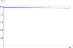
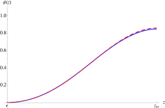
Figure 1: Figures (a) and (b) display the numerical solutions to Eq. (37) for $\psi(z)$ and $\phi(z)$, respectively. In both figures there are two curves plotted: the blue curves are the numerical solutions and the red, dashed curves are the approximate solutions ($\psi(z)=1$ in figure (a) and $\phi=[1-A(0,z)]$ in figure (b)). These plots were made with $m_{q}=2.36\ {\rm MeV}$ and $\sigma=(333\ {\rm MeV})^{3}$.

The functions $\psi(z)$ and $\phi(z)$ are normalized to obtain a canonically normalized kinetic term in the low energy theory. The plotted numerical solutions illustrate the extent to which the approximations of the previous section are valid.

We would also like to understand numerically how robust the GOR relation is in this model, with respect to varying some of the parameters. In particular, fixing $m_{\pi}=140\ {\rm MeV}$ (by adjusting $m_{q}$ for fixed values of $\sigma$) we would like to see what happens for different values of $\sigma$. Varying the condensate by sampling a discrete number of points from $(290\ {\rm MeV})^{3}$ to $(360\ {\rm MeV})^{3}$, the pion decay constant takes values ranging from $79\ {\rm MeV}$ to $102\ {\rm MeV}$ and the quark mass goes from $2.52\ {\rm MeV}$ down to $2.21\ {\rm MeV}$. In Fig. 2, we plot the ratio $(m_{\pi}^{2}f_{\pi}^{2})/(2m_{q}\sigma)$ for the above specified range of values for the condensate. If the GOR relation holds, the ratio should be approximately 1 and we can see that the plot shows good agreement over the entire region.

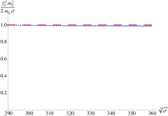
Figure 2: The red long-dashed line is a horizontal line at 1. The blue dots are the values of the function, $(m_{\pi}^{2}f_{\pi}^{2})/(2m_{q}\sigma)$. For this plot, the quark mass is adjusted to fix $m_{\pi}=140\ {\rm MeV}$ at each point.

VI Consequences for Holographic QCD

We check that the change of background does not adversely affect some standard predictions of the hard-wall model; that is, we will compare our predictions with those of “Model A” in Ref. Erlich:2005qh . We might expect the modifications to be marginal because only the pion physics should be sensitive to changes in $m_{q}$, but we have also changed a sign. Aside from the substitution $\tilde{m}_{q}\rightarrow-2m_{q}$, the derivations of the equations of motion for the gauge fields and of the vector current correlators are unaffected by the new form of the $X$-field. Since the expressions for the related observables we compute are likewise unchanged, we refer the reader to Ref. Erlich:2005qh , for more detail. In the following, we summarize the methods for obtaining the results. To calculate the mass of the $a_{1}$, we solve Eq. (35) for the normalizable mode $\psi_{a_{1}}(z)$ with boundary conditions $\psi_{a_{1}}(\epsilon)=\partial_{z}\psi_{a_{1}}(z_{m})=0$. The wavefunction $\psi_{a_{1}}$ is normalized such that $A_{\mu}(x)$ has a canonical kinetic term, where $A_{\mu}(x,z)=\psi_{a_{1}}(z)A_{\mu}(x)$ . As derivable from the two-point vector current correlator, we use the following expression to calculate the decay constants in terms of the profile in the extra dimension: $F^{1/2}=\sqrt{\psi^{\prime\prime}(0)/g_{5}}$. And finally, by looking at the terms cubic in the fields, coupling $V\pi\pi$, we make a prediction for $g_{\rho\pi\pi}$. All relevant cubic terms are the following:

$${\cal S}\supset\epsilon^{abc}\int d^{5}x\ V_{\mu}^{b}\left[\frac{1}{zg_{5}^{2}}\partial_{z}\partial^{\mu}\phi^{a}\partial_{z}\phi^{c}+\frac{1}{z^{3}}\partial^{\mu}\left(v\phi^{a}-\sigma z^{3}\pi^{a}\right)\left(v\phi^{c}-\sigma z^{3}\pi^{c}\right)\right],$$ (42)

where we have used the equations of motion for the vector field to obtain this expression. In order to calculate the on-shell $g_{\rho\pi\pi}$ from the effective 4D theory, we integrate out the extra dimension and identify $g_{\rho\pi\pi}$ as the coefficient of $\epsilon^{abc}\partial^{\mu}\pi^{a}(x)\rho_{\mu}^{b}(x)\pi^{c}(x)$, where $\rho_{\mu}^{b}$ is the lowest mode in the vector field KK decomposition. Extracting this coefficient from Eq. (42) we find

$$g_{\rho\pi\pi}=\frac{g_{5}}{f_{\pi}^{2}}\int dz\ \psi_{\rho}(z)\left[\frac{1}{zg_{5}^{2}}(\partial_{z}\phi)^{2}+\frac{1}{z^{3}}\left(v\phi-\sigma z^{3}\psi\right)^{2}\right],$$ (43)

where the $z$-integral of the expression in brackets is normalized to $f_{\pi}^{2}$. The results are presented in Table 1 and we find that the new predictions have not changed significantly compared to “Model A” – they are still on the $10\%$ level, with the exception of $g_{\rho\pi\pi}$.

Observable	Measured (MeV)	Model (MeV)	Model A (MeV)Erlich:2005qh
$m_{\pi}$	140	140	140
$m_{\rho}$	776	776	776
$m_{a_{1}}$	1230	1370	1360
$f_{\pi}$	92.4	92.0	92.4
$F_{\rho}^{1/2}$	345	329	329
$F_{a_{1}}^{1/2}$	433	493	486
$g_{\rho\pi\pi}$	6.03	4.44	4.48

Table 1: The predictions of the model as compared with “Model A” and experimental values Erlich:2005qh . The results are based on fitting to $m_{\pi}$, $f_{\pi}$, and $m_{\rho}$, leading to the parameter choice $m_{q}=2.36\ {\rm MeV}$, $\sigma=(333\ {\rm MeV})^{3}$, and $z_{m}=1/(323\ {\rm MeV})$.

VII Conclusions

Holographic QCD models are surprisingly successful in their predictions of low-energy QCD observables. However, it was discovered in earlier work that the pion condensation transition in one version of the hard-wall model has qualitatively different features than the predictions of chiral perturbation theory and other approaches. We have shown that this disagreement is due to a boundary effect related to the explicit breaking of the gauged chiral symmetry by the non-normalizable background of a 5D scalar field. To restore agreement with the chiral Lagrangian we modified the boundary dynamics, either by introducing nonlinear boundary conditions on the fields, or by performing a nonlinear field redefinition which induced an infrared boundary term in the action. The field redefinition allowed us to relate the system with nonlinear boundary conditions to a standard Sturm-Liouville system which manifestly maintains the proper symmetry structure, justifying the subsequent Kaluza-Klein decomposition of the fields. The chirally improved hard-wall model makes predictions for low-energy QCD observables that agree with the original model to within 1-2%.

It would be useful to further explore the consequences of the modified boundary physics with regard to pion observables. It would also be interesting to find additional applications of nonlinear boundary conditions to extra-dimensional model building, for example to Higgsless models and holographic technicolor models. Finally, the necessity for nonlinear boundary dynamics in the hard-wall model provides motivation for further study of the mathematical problem of differential equations with nonlinear boundary conditions. In particular, it would be useful to classify those systems of equations and boundary conditions that can be related to a Sturm-Liouville system by a change of variables.

- (1) C. Csaki, H. Ooguri, Y. Oz and J. Terning, JHEP 9901, 017 (1999) [hep-th/9806021].
- (2) J. Polchinski and M. J. Strassler, arXiv:hep-th/0003136.
- (3) S. J. Brodsky and G. F. de Teramond, Phys. Lett. B 582, 211 (2004) [arXiv:hep-th/0310227].
- (4) G. F. de Teramond and S. J. Brodsky, Phys. Rev. Lett. 94, 201601 (2005) [arXiv:hep-th/0501022].
- (5) J. Erlich, E. Katz, D. T. Son and M. A. Stephanov, Phys. Rev. Lett. 95, 261602 (2005) [arXiv:hep-ph/0501128].
- (6) L. Da Rold and A. Pomarol, Nucl. Phys. B 721, 79 (2005) [arXiv:hep-ph/0501218].
- (7) J. M. Maldacena, Adv. Theor. Math. Phys. 2, 231 (1998) [Int. J. Theor. Phys. 38, 1113 (1999)] [arXiv:hep-th/9711200].
- (8) E. Witten, Adv. Theor. Math. Phys. 2, 253 (1998) [arXiv:hep-th/9802150].
- (9) S. S. Gubser, I. R. Klebanov and A. M. Polyakov, Phys. Lett. B 428, 105 (1998) [arXiv:hep-th/9802109].
- (10) T. Sakai and S. Sugimoto, Prog. Theor. Phys. 113, 843 (2005) [arXiv:hep-th/0412141]; T. Sakai and S. Sugimoto, Prog. Theor. Phys. 114, 1083 (2005) [arXiv:hep-th/0507073].
- (11) V. Balasubramanian, P. Kraus and A. E. Lawrence, Phys. Rev. D 59, 046003 (1999) [hep-th/9805171].
- (12) I. R. Klebanov and E. Witten, Nucl. Phys. B 556, 89 (1999) [hep-th/9905104].
- (13) J. Erlich and C. Westenberger, Phys. Rev. D 79, 066014 (2009) [arXiv:0812.5105 [hep-ph]].
- (14) Z. Abidin and C. E. Carlson, Phys. Rev. D 80, 115010 (2009) [arXiv:0908.2452 [hep-ph]].
- (15) C. Csaki, M. Reece and J. Terning, JHEP 0905, 067 (2009) [arXiv:0811.3001 [hep-ph]].
- (16) M. Shifman, hep-ph/0507246.
- (17) A. Karch, E. Katz, D. T. Son and M. A. Stephanov, Phys. Rev. D 74, 015005 (2006) [hep-ph/0602229].
- (18) D. Albrecht and J. Erlich, Phys. Rev. D 82, 095002 (2010) [arXiv:1007.3431 [hep-ph]].
- (19) A. B. Migdal, O. A. Markin and I. N. Mishustin, Zh. Eksp. Teor. Fiz. 70, 1592 (1976).
- (20) R. F. Sawyer and D. J. Scalapino, Phys. Rev. D 7, 953 (1973).
- (21) D. B. Kaplan and A. E. Nelson, preprint HUTP-86/A023; Phys. Lett. B 175, 57 (1986).
- (22) D. T. Son and M. A. Stephanov, Phys. Rev. Lett. 86, 592 (2001) [arXiv:hep-ph/0005225]; D. T. Son and M. A. Stephanov, Phys. Atom. Nucl. 64, 834 (2001) [Yad. Fiz. 64, 899 (2001)] [arXiv:hep-ph/0011365].
- (23) J. B. Kogut and D. K. Sinclair, Phys. Rev. D 66, 034505 (2002) [arXiv:hep-lat/0202028].
- (24) P. de Forcrand, M. A. Stephanov and U. Wenger, PoS LAT2007, 237 (2007) [arXiv:0711.0023 [hep-lat]].
- (25) W. Detmold, M. J. Savage, A. Torok, S. R. Beane, T. C. Luu, K. Orginos and A. Parreno, Phys. Rev. D 78, 014507 (2008) [arXiv:0803.2728 [hep-lat]].
- (26) W. Detmold, K. Orginos, M. J. Savage and A. Walker-Loud, Phys. Rev. D 78, 054514 (2008) [arXiv:0807.1856 [hep-lat]].
- (27) R. Wilcox, “The Pion in AdS/QCD,” Thesis (B.S.), College of William and Mary (2011).
- (28) O. Domenech, G. Panico and A. Wulzer, Nucl. Phys. A 853, 97 (2011) [arXiv:1009.0711 [hep-ph]].
- (29) E. Witten, hep-th/0112258.
- (30) M. Berkooz, A. Sever and A. Shomer, JHEP 0205, 034 (2002) [hep-th/0112264].
- (31) C. D. Carone and H. Georgi, Phys. Rev. D 49, 1427 (1994) [hep-ph/9308205].
- (32) C. D. Carone, J. Erlich and J. A. Tan, Phys. Rev. D 75, 075005 (2007) [hep-ph/0612242].
- (33) A. Cherman, T. D. Cohen and E. S. Werbos, Phys. Rev. C 79, 045203 (2009) [arXiv:0804.1096 [hep-ph]].
- (34) L. Da Rold and A. Pomarol, JHEP 0601, 157 (2006) [hep-ph/0510268].
- (35) T. M. Kelley, S. P. Bartz and J. I. Kapusta, Phys. Rev. D 83, 016002 (2011) [arXiv:1009.3009 [hep-ph]].
- (36) G. Panico and A. Wulzer, JHEP 0705, 060 (2007) [hep-th/0703287].
- (37) C. Csaki, C. Grojean, H. Murayama, L. Pilo and J. Terning, Phys. Rev. D 69, 055006 (2004) [hep-ph/0305237].