Bayesian model choice and information criteria in sparse generalized linear models

Abstract.

We consider Bayesian model selection in generalized linear models that are high-dimensional, with the number of covariates $p$ being large relative to the sample size $n$, but sparse in that the number of active covariates is small compared to $p$. Treating the covariates as random and adopting an asymptotic scenario in which $p$ increases with $n$, we show that Bayesian model selection using certain priors on the set of models is asymptotically equivalent to selecting a model using an extended Bayesian information criterion. Moreover, we prove that the smallest true model is selected by either of these methods with probability tending to one. Having addressed random covariates, we are also able to give a consistency result for pseudo-likelihood approaches to high-dimensional sparse graphical modeling. Experiments on real data demonstrate good performance of the extended Bayesian information criterion for regression and for graphical models.

1. Introduction

Information criteria provide a principled approach to a wide variety of model selection problems. The criteria strike a balance between the fit of a parametric statistical model, measured by the maximized likelihood function, and its complexity, measured by a penalty term that involves the dimension of the model’s parameter space. The two classical criteria are Akaike’s information criterion (AIC) (Akaike, 1974), which targets good predictive performance, and the Bayesian information criterion (BIC) introduced in Schwarz (1978), which is motivated by a connection to fully Bayesian approaches to model determination and which has been proven to enjoy consistency properties in a number of settings. If we call a model “true” if it contains the underlying data-generating distribution, then consistency refers to selection of the smallest true model in a suitable large-sample limit. In this paper we will be concerned with the BIC for generalized linear models with random covariates in a sparse high-dimensional setting, where the number of covariates is large but only a small fraction of the covariates is related to the response. Our main results show that extensions of the BIC are consistent, and are accurate approximations of Bayesian procedures, in asymptotic scenarios where the number of covariates grows with the sample size. The results can be interpreted either as giving a precise Bayesian motivation for recently-proposed information criteria, or as proving that Bayesian procedures enjoy favorable frequentist properties. In particular, our work gives uniform error bounds for Laplace approximations to the large number of marginal likelihood integrals arising in a Bayesian treatment of sparse high-dimensional generalized linear models, and results in consistent model selection for high-dimensional graphical models with binary variables (the Ising model).

1.1. Classical theory

Suppose we observe a sample of $n$ observations for which we consider the parametric model $\mathcal{M}$ with log-likelihood function $\ell_{[n]}(\theta)$. Then, written in the most commonly encountered form, the BIC for this model is

$$\mathrm{BIC}(\mathcal{M})=-2\,\ell_{[n]}(\widehat{\theta}_{\mathcal{M}})+\dim(\mathcal{M})\cdot\log(n)\;,$$

with a lower value being desirable. Here $\dim(\mathcal{M})$ is the dimension of the model’s parameter space $\Theta_{\mathcal{M}}$, and

$$\widehat{\theta}_{\mathcal{M}}=\arg\max_{\theta\in\Theta_{\mathcal{M}}}\,\ell_{[n]}(\theta)$$

is the maximum likelihood estimator (MLE) in model $\mathcal{M}$. The classical large-sample theory underlying the BIC considers a finite family of competing models that is closed under intersection, and for which strict inclusion implies strictly lower dimension. In order to prove consistency of the BIC, it then suffices to make pairwise comparisons between models $\mathcal{M}_{1}$ and $\mathcal{M}_{2}$ showing that, with asymptotic probability one, $\mathrm{BIC}(\mathcal{M}_{1})<\mathrm{BIC}(\mathcal{M}_{2})$ if either (i) $\mathcal{M}_{1}$ is true and $\mathcal{M}_{2}$ is not, or (ii) both $\mathcal{M}_{1}$ and $\mathcal{M}_{2}$ are true but $\dim(\mathcal{M}_{1})<\dim(\mathcal{M}_{2})$. In case (i), a proof shows that the difference in the likelihood terms in the BIC outgrows the logarithmic penalty term as $n\to\infty$, whereas in case (ii) the logarithmic term outgrows the difference in log-likelihood values, which remains bounded in probability; compare, for instance, Nishii (1984), Haughton (1988) or monographs on model selection and information criteria such as Burnham and Anderson (2002); Claeskens and Hjort (2008); Konishi and Kitagawa (2008).

The penalty term appearing in the BIC is only one of many possible choices to balance model fit and complexity in a way that leads to consistency. However, the logarithmic dependence on the sample size makes a connection to Bayesian approaches. Consider the prior $f_{\mathcal{M}}(\theta)$ for the parameter $\theta$ in model $\mathcal{M}$, and write $P(\mathcal{M})$ for the prior probability of $\mathcal{M}$. Then the posterior probability of $\mathcal{M}$ is proportional to

(1) $$P(\mathcal{M})\cdot\int_{\theta}\exp\{\ell_{[n]}(\theta)\}\,f_{\mathcal{M}}(\theta)\;d\theta,$$

where the integral is commonly referred to as the marginal likelihood. In well-behaved models, for large $n$, the integrand in the marginal likelihood takes large values only in a neighborhood of the MLE $\widehat{\theta}_{\mathcal{M}}$. Moreover, in such a neighborhood the log-likelihood $\ell_{[n]}(\theta)$ can be approximated by a quadratic function, while the prior $f_{\mathcal{M}}(\theta)$ is approximately constant. Evaluating the resulting Gaussian integral reveals that the logarithm of the marginal likelihood equals $-\nicefrac{{1}}{{2}}\cdot\mathrm{BIC}(\mathcal{M})$ plus a remainder term that is bounded in probability when the $n$ observations are drawn from a distribution in $\mathcal{M}$ and the sample size $n$ tends to $\infty$. The remainder term can be estimated to be

$$\frac{1}{2}\dim(\mathcal{M})\log(2\pi)+\log f_{\mathcal{M}}(\widehat{\theta}_{\mathcal{M}})-\frac{1}{2}\log\det\left(\frac{1}{n}H_{[n]}(\widehat{\theta}_{\mathcal{M}})\right)+\mathbf{O}_{P}(n^{-1/2}),$$

where $H_{[n]}$ is the Hessian of the negated log-likelihood function (and scales with $n$). The work of Haughton (1988) provides a rigorous probabilistic treatment of this Laplace approximation to the marginal likelihood in the general setting of smooth (or curved) exponential families. Considering a finite family of models, it suffices to treat one model at a time in this analysis.

1.2. Recent extensions of the BIC

In the last decade, new applications of the BIC have emerged in problems of selecting sparse models for high-dimensional data, including problems such as tuning parameter selection in Lasso and related regularization procedures; see e.g. Zou et al. (2007). Following a proposal from Bogdan et al. (2004), the work of Chen and Chen (2008) treats an extended BIC for variable selection in sparse high-dimensional linear regression with deterministic covariates. The extension allows for a more stringent penalty to address the (ordinary) BIC’s tendency to select overly large models in this setting. The asymptotic scenario underlying the theoretical analysis of the new criterion allows for subexponential growth in the number of covariates $p$ as a function of the sample size $n$, with a bound on the number of covariates that appear in the true mean function. The main result of Chen and Chen (2008) shows variable selection consistency under these asymptotics. Chen and Chen (2011) extend the results to generalized linear models (GLMs), and further improvements for linear regression are given in Luo and Chen (2011a) and in Zhang and Shen (2010). Consistency in Gaussian graphical models has been studied by Foygel and Drton (2010) and Gao et al. (2011). Composite likelihood-based criteria are treated by Gao and Song (2010). The main difficulty in showing consistency in these high-dimensional settings is the need to control a diverging number of models. We remark that a related study of the ordinary BIC that focuses on pairwise model comparisons is given by Moreno et al. (2010).

In the literature on the extended BIC, the key idea for treating the high-dimensional setting is to augment the BIC with an informative prior on models. In the regression setting, which is our focus in this paper, the competing models correspond to different subsets of covariates. If $p$ denotes the number of covariates, then a model corresponds to a subset ${J}\subset[p]\coloneqq\{1,\dots,p\}$, and the extended BIC is based on the prior

(2) $$P(J)=\frac{1}{p+1}{p\choose|J|}^{-1}$$

that gives equal probability to each model size, and to each model given the size. Clearly, this priors favors an individual small model over an individual model of moderate size. More generally, priors of the form

(3) $$P(J)\propto{p\choose|J|}^{-\gamma}\cdot{\mathbbm{1}}\left\{{|J|\leq q}\right\}$$

with a hyperparameter $\gamma\in[0,1]$ have been considered to allow one to interpolate between the classical BIC of Schwarz (1978), obtained for $\gamma=0$, and the prior in (2) given by $\gamma=1$, while at the same time invoking an upper bound $q$ on the number of covariates. Some of our later asymptotic results suggest that it can be useful to consider $\gamma>1$ if the number of covariates $p$ is very large. Priors of this form have also been shown to be useful in fully Bayesian approaches to high-dimensional regression; compare Scott and Berger (2010) who motivate this and related priors in a construction that includes each covariate with a fixed probability that itself is given a Beta prior.

Writing $J$ for a particular subset of the available covariates, inclusion of the prior from (3) into the information criterion yields the extended BIC (EBIC)

$$\mathrm{BIC}_{\gamma}(J)=-2\ell_{[n]}(\widehat{\theta}_{J})+|J|\cdot\log(n)+2\gamma|J|\cdot\log(p)\,.$$

Under suitable conditions on the design matrix (ensuring, for instance, that removing a covariate from the smallest true model will substantially lower the achievable likelihood), Chen and Chen (2008, 2011) show consistency of the EBIC in both the normal linear regression and the univariate GLM setting with fixed (i.e., non-random) covariates. Consistency holds as long as $\gamma>1-\frac{1}{2\kappa}$, where $\kappa$ determines the rate of growth of the number of covariates, and thus the space of possible models, with $p=\mathbf{O}(n^{\kappa})$.

While our focus is entirely on consistency properties of model selection procedures for high-dimensional regression, we should mention that other properties are of interest and have been studied. For instance, Shao (1997) considers a similar problem, proving results about selection of the best predictive model, rather than consistency in variable selection. Jiang (2007) points out that in applied settings, the question of variable selection is not always well-defined due to many coefficients that are approximately rather than exactly zero, and considers the problem of estimating the true parameter vector under the assumption of approximate sparsity. This paper uses a prior on models similar to the one in (2).

1.3. Recent work on Bayesian model selection in high-dimensional settings

Several recent papers have examined the properties of Bayesian model selection in scenarios where the model size may be large relative to the sample size. For instance, a consistency result for Bayesian linear regression has recently been obtained by Shang and Clayton (2011). This work focuses on a specific Bayesian model that assumes the regression coefficients to follow a particular prior distribution that is a mixture of a normal distribution and a point mass at zero. There has also been work on the problem of choosing between a pair of models, including a recent article by Kundu and Dunson (2011) that shows consistency of Bayesian pairwise model comparison under a flexible, non-parametric noise model. These results are not directly comparable to the problem discussed here, where we consider the problem of searching for the smallest true model from among a combinatorially large set of possible sparse models in a generic regression setting.

1.4. New results

With a penalty term reflecting a particular type of prior on models, the EBIC has a clear Bayesian motivation. However, it is not immediately clear that the EBIC and fully Bayesian approaches using the same prior on models should lead to asymptotically equivalent model choice in a high-dimensional asymptotic scenario that has the number of covariates $p$ grow with the sample size $n$. Our first main result, Theorem 1, addresses this issue for generalized linear models and shows that such equivalence indeed occurs at a fairly general level. More precisely, our result shows that a Laplace approximation to the marginal likelihood of each one of a growing number of models results into errors that are, with high probability, uniformly bounded as $\mathbf{O}\big{(}\sqrt{{\log(np)}/{n}}\big{)}$.

Our second main result, Theorem 2, provides a consistency result for the EBIC. The result is very closely related to those of Chen and Chen (2011). The primary difference is that we consider random rather than deterministic covariates and allow for unbounded covariates, subject to a moment condition, in some special cases such as logistic regression. Consistency is proven under the same conditions that we use to obtain the equivalence of the EBIC and fully Bayesian model selection. Combining the two Theorems yields Corollary 1, which states consistency for fully Bayesian model determination.

Theorem 2 also allows us to obtain consistency results for pseudo-likelihood methods in graphical model selection, where regressions are performed to model each node’s dependence on the other nodes in the graph (“neighborhood selection” for each node), and these neighborhoods are then combined to hypothesize a sparse graphical model; see Meinshausen and Bühlmann (2006) and Ravikumar et al. (2010). Since in each regression, the covariates consist of random observations from the potential “neighbors” of the node in question, it is crucial that our analysis of consistency allows for random covariates. Furthermore, for consistent model selection, the neighborhood selection procedure must succeed simultaneously for each node, and therefore we make use of the explicitly-calculated finite-sample bounds in Theorem 2. Our results for the graphical Ising model are given in Theorem 4.

The remainder of this paper is organized as follows. We begin by defining the setting and introducing notation, in Section 2. In Section 3, we discuss Bayesian model selection and the Laplace approximation to the marginal likelihood. Our result on the consistency of the EBIC for regression is given in Section 4, where we also present experiments on real data that show good performance of the EBIC in practice. In Section 5, we turn to graphical models and present theoretical and empirical results showing the consistency of the EBIC for reconstructing a sparse graph based on a neighborhood selection procedure. We outline the proofs for Theorems 1 , 2, and 4 in Section 6, and give the full proofs in the Appendix. Finally, in Section 7, we discuss our results and outline directions for future work.

2. Setup and assumptions

We treat generalized linear models in which the observations of the response variable follow a distribution from a univariate exponential family with densities

$$p_{\theta}(y)\,\propto\,\exp\left\{y\cdot\theta-\mathbf{b}(\theta)\right\}\,,\qquad\theta\in\Theta=\mathbb{R},$$

where the density is defined with respect to some measure on $\mathbb{R}$. More precisely, the observations of the response are independent random variables $Y_{1},\dots,Y_{n}$, with $Y_{i}\sim p_{\theta_{i}}$. The vector of natural parameters $\boldsymbol{\theta}=(\theta_{1},\dots,\theta_{n})^{T}$ is assumed to lie in the linear space spanned by the columns of a design matrix $X=(X_{ij})\in\mathbb{R}^{n\times p}$, that is, $\boldsymbol{\theta}=X\phi$ for some parameter vector $\phi\in\mathbb{R}^{p}$. Our focus is on the case of random covariates. Let $X_{\scriptscriptstyle\bullet j}$ be the $n$-dimensional vector of observed values for the $j$th covariate (the $j$th column of the design matrix $X$), and write $X_{i\scriptscriptstyle\bullet}$ for the $p$-dimensional covariate vector in the $i$th row of the design matrix $X$. Then we assume $X_{1\scriptscriptstyle\bullet},\dots,X_{n\scriptscriptstyle\bullet}$ to be independent and identically distributed random vectors.

Our results treat a sparsity scenario in which the joint distribution of $Y_{1},\dots,Y_{n}$ is determined by a true parameter vector $\phi^{*}\in\mathbb{R}^{p}$ supported on a (small) set $J^{*}\subset[p]$, that is, $\phi^{*}_{j}\not=0$ if and only if $j\in J^{*}$. Our interest is in recovery of the set $J^{*}$. To this end, we consider the different submodels given by the linear spaces spanned by subsets $J\subset[p]$ of the columns of the design matrix $X$. We will use $J$ to denote either an index set for covariates or the resulting model, for convenience. Finally, we denote subsets of covariates by $X_{iJ}=(X_{ij})_{j\in J}$, where $J\subset[p]\coloneqq\{1,\dots,p\}$.

2.1. Assumptions

We will be concerned with asymptotic questions in a scenario in which $n\rightarrow\infty$ and the number of covariates $p=p_{n}$ is allowed to grow. Let $\kappa_{n}=\log_{n}(p_{n})$, and let $\kappa=\lim\sup\kappa_{n}\in[0,\infty]$. Subsequently, we will suppress the sample size index and write $p$ rather than $p_{n}$. Our theorems apply to either one of the following cases (recall that $X_{1j},\dots,X_{nj}$ are identically distributed):

• The covariates are bounded (or bounded with probability one), that is, there is a constant $\mathbf{A}<\infty$ such that, $|X_{1j}|\leq\mathbf{A}$ for $j=1,\dots,p$.

• There is an even integer $K>2\kappa$ (in particular, $\kappa<\infty$), for which the covariates have moments bounded as $\mathbb{E}\left[|X_{1j}|^{6K}\right]\leq\mathbf{A}_{K}<\infty$ for $j=1,\dots,p$. Moreover, for all $t>0$, it holds that

  $$\mathbf{B}_{K}(t)\coloneqq\sup_{j}\mathbb{E}_{X_{1j}}\left[\sup_{|\theta|\leq t|X_{1j}|}\left|\mathbf{b}^{\prime\prime\prime}(\theta)\right|^{2K}\right]<\infty\;.$$

We remark that the condition on the third derivative of the cumulant generating function $\mathbf{b}$ holds for logistic and Poisson models, as well as the normal model with known variance. In addition, we assume the following five conditions:

• The growth of $p$ is subexponential, that is, $\log(p)=\mathbf{o}(n)$.

• The size of the true model given by the cardinality of the support $J^{*}$ of the true parameter vector $\phi^{*}$ is bounded as $|J^{*}|\leq q$ for a fixed integer $q\in\mathbb{N}$.

• All small sets of covariates have second moment matrices with bounded eigenvalues, that is, for some fixed finite constants $a_{1},a_{2}>0$, it holds that $a_{1}\mathbf{I}_{J}\preceq\mathbb{E}\left[X_{1J}X_{1J}^{T}\right]\preceq a_{2}\mathbf{I}_{J}$ for all $|J|\leq 2q$.

• The norm of the true signal is bounded, namely, $\|\phi^{*}\|_{2}\leq a_{3}$ for a fixed constant $0<a_{3}<\infty$.

• The small true coefficients have bounded decay such that

  $$\sqrt{\frac{\log(np)}{n}}=\mathbf{o}\left(\min\left\{\left|\phi^{*}_{j}\right|:j\in J^{*}\right\}\right).$$

2.2. Comparison to assumptions used in existing work

We compare the above assumptions to those used by Chen and Chen (2011), who show that the EBIC is consistent for univariate GLMs with fixed covariates. In this work by Chen and Chen, only bounded covariates are considered — that is, our (A1) scenario. Our conditions (B1), (B2), and (B4) appear (explicitly or implicitly) in their work as well. Condition (B5) appears in a stronger form in their work, where they assume that $\phi^{*}$ is fixed and therefore its minimal nonzero value is bounded from below by some constant.

A crucial difference lies in our assumption (B3). The analogous condition of Chen and Chen (2011) requires that, for some positive finite $\lambda_{1}$ and $\lambda_{2}$, $\lambda_{1}\mathbf{I}_{J}\preceq n^{-1}H_{J}(\phi_{J})\preceq\lambda_{2}\mathbf{I}_{J}$, for any $J\supset J^{*}$ with $|J|\leq 2q$ and any $\phi_{J}$ in a neighborhood of $\phi^{*}_{J}$. Here $H_{J}(\cdot)\coloneqq\left(H_{[n]}(\cdot)\right)_{J,J}$ is the Hessian of the negative log-likelihood function (restricted to rows and columns corresponding to the covariates in $J$). Note that $H_{J}(\cdot)$ depends on the design matrix $X_{J}$ for the given set of covariates $J$. Since we work in the setting of random covariates, we cannot make this assumption on the empirical design matrix, and therefore use condition (B3), which is a weaker assumption on the distribution of the covariates.

3. Bayesian model selection

Observing the independent random vectors $(X_{1\scriptscriptstyle\bullet},Y_{1}),\dots,(X_{n\scriptscriptstyle\bullet},Y_{n})$, the likelihood function of the considered GLM is

$$L_{[n]}(\phi)=\exp\left\{\ell_{[n]}(\phi)\right\}=\exp\left\{\sum_{i=1}^{n}\ell_{i}(\phi)\right\}=\exp\left\{\sum_{i=1}^{n}Y_{i}\cdot X_{i\scriptscriptstyle\bullet}^{T}\phi-\mathbf{b}(X_{i\scriptscriptstyle\bullet}^{T}\phi)\right\}\;,$$

with $\ell_{i}(\phi)$ being the log-likelihood function based on the $i$th observation $(X_{i\scriptscriptstyle\bullet},Y_{i})$. Let $P(J)$ be the prior probability of model $J\subset[p]$, and let $f_{J}(\phi_{J})$ be a prior density on the model’s parameter space $\mathbb{R}^{J}$. The unnormalized posterior probability of model $J$ is then

$$\mathrm{Bayes}(J)=P(J)\cdot\int_{\phi_{J}\in\mathbb{R}^{J}}L_{[n]}(\phi_{J})f_{J}(\phi_{J})\;d\phi_{J}\;,$$

where, with some abuse of notation, we write $L_{[n]}(\phi_{J})$ for the likelihood function of the model given by $J\subset[p]$, that is,

$$L_{[n]}(\phi_{J})=\exp\left\{\sum_{i=1}^{n}\ell_{i}(\phi_{J})\right\}=\exp\left\{\sum_{i=1}^{n}Y_{i}\cdot X_{iJ}^{T}\phi_{J}-\mathbf{b}(X_{iJ}^{T}\phi_{J})\right\}.$$

Our interest is now in the frequentist properties of the Bayesian model selection procedure that chooses a model $J$ by maximizing the (unnormalized) posterior probability $\mathrm{Bayes}(J)$. Assuming that observations are drawn from a distribution in the GLM, we ask the following two questions. First, is the Bayesian procedure consistent, that is, will it choose the smallest true model in the large-sample limit? Second, how can we approximate the marginal likelihood integral appearing in $\mathrm{Bayes}(J)$, without introducing approximation errors that might change which model is selected? In the classical scenario with a fixed number of covariates $p$, when considering a growing sample size $n$, the answers to the above questions are tied together. Under suitable conditions, consistency of the Bayesian procedure can be established by proving that, for large samples, it selects the same model as the consistent BIC or the more accurate approximation obtained by applying the Laplace approximation to the marginal likelihood integral. We will show these same connections to exist in sparse high-dimensional settings.

Theorem 1 below states that, under appropriate conditions, the Laplace approximation to marginal likelihood integrals remains uniformly accurate across large spaces of models. This result is obtained under an upper bound $q$ on the model size. As discussed in Section 1.2 in the introduction, we give special emphasis to a particular class of prior distributions on the set of models, namely, priors of the form

(4) $$P(J)\propto{p\choose|J|}^{-\gamma}\cdot{\mathbbm{1}}\left\{{|J|\leq q}\right\}\;,\qquad J\subset[p],$$

for some $\gamma\geq 0$. We write $\mathrm{Bayes}_{\gamma}(J)$ for the unnormalized posterior probability associated with the choice of prior $P(J)={p\choose|J|}^{-\gamma}\cdot{\mathbbm{1}}\left\{{|J|\leq q}\right\}$, where we suppress the normalizing constant in the prior for convenience. Then we show that, for sufficiently large $n$, the event

$$\arg\min_{|J|\leq q}\mathrm{BIC}_{\gamma}(J)=\arg\max_{|J|\leq q}\mathrm{Bayes}_{\gamma}(J)\;.$$

occurs with high probability. In other words, the EBIC

(5) $$\mathrm{BIC}_{\gamma}(J)=-2\log L_{[n]}(\widehat{\phi}_{J})+|J|\log(n)+2\gamma|J|\log(p)\;.$$

yields an approximation to the Bayesian posterior probability that is accurate enough for the resulting model selection procedures to be asymptotically equivalent. In fact, Theorem 1 states a stronger result according to which $\mathrm{Bayes}_{\gamma}(J)$ is approximated up to a constant by $\mathrm{BIC}_{\gamma}(J)$. Finally, we prove consistency of the EBIC in Section 4. In combination with the results of this section, we obtain a proof of the consistency of the Bayesian model selection procedure.

We now give the precise statement of the points just outlined. We adopt the notation $a=b(1\pm c)$ to conveniently express that $a$ belongs to the interval $[b(1-c),b(1+c)]$.

Theorem 1.

Assume that conditions (B1)-(B5) hold, and that either assumption (A1) or (A2) holds. Moreover, assume the following mild conditions on the family of priors $\left(f_{J}:J\subset[p],|J|\leq q\right)$, which require the existence of constants $0<F_{1},F_{2},F_{3}<\infty$ such that, uniformly for all $|J|\leq q$, we have

• an upper bound on the priors:

  $$\sup{}_{\phi_{J}}f_{J}(\phi_{J})\leq F_{1}<\infty,$$

• a lower bound on the priors over a compact set:

  $$\inf{}_{\|\phi_{J}\|_{2}\leq R+1}f_{J}(\phi_{J})\geq F_{2}>0,$$

  where $R$ is a function of the constants in assumptions (A1) or (A2) and (B1)-(B5), defined in the proofs,

• a Lipschitz property on the same compact set:

  $$\sup{}_{\|\phi_{J}\|_{2}\leq R+1}\left\|\nabla f_{J}(\phi_{J})\right\|_{2}\leq F_{3}<\infty.$$

Then there is a constant $C$, no larger than $4F_{3}F_{2}^{-1}\lambda_{1}^{-\nicefrac{{1}}{{2}}}+2q\lambda_{3}\lambda_{1}^{-\nicefrac{{3}}{{2}}}+2$, such that, for sufficiently large $n$, the event that

$$\mathrm{Bayes}(J)=P(J)\cdot L_{[n]}(\widehat{\phi}_{J})f_{J}(\widehat{\phi}_{J})\cdot\left|H_{J}(\widehat{\phi}_{J})\right|^{-\nicefrac{{1}}{{2}}}(2\pi)^{\nicefrac{{|J|}}{{2}}}\cdot\left(1\pm C\sqrt{\frac{\log(np)}{n}}\right)\text{ for all }|J|\leq q$$

occurs with probability at least $1-(np)^{-1}$ under (A1), and with probability at least $1-(np)^{-1}-4K^{K+1}n^{-\frac{K-2\kappa}{2}}$ under (A2). In particular, for the (unnormalized) prior $P(J)={p\choose|J|}^{-\gamma}\cdot{\mathbbm{1}}\left\{{|J|\leq q}\right\}$, it holds that

$$\left|\log\left(\mathrm{Bayes}_{\gamma}(J)\right)-\left(-\tfrac{1}{2}\mathrm{BIC}_{\gamma}(J)\right)\right|\leq C_{1}\;,$$

where $C_{1}$ is a constant no larger than $\tfrac{q}{2}\log(2\pi)+\gamma q\log(2q)+q\log\max\{\lambda_{1}^{-1},\lambda_{2}\}+\log\max\{F_{1},F_{2}^{-1}\}+1$.

The proof of this theorem is given in Section 6. The constant $R$ appearing in conditions (ii) and (iii) on the family of priors arises in the proof, where we show that with high probability, the MLEs $\widehat{\phi}_{J}$ for all sparse models $J$ will lie inside a ball of radius $R$ centered at zero.

4. Consistency of the extended Bayesian information criterion

Let $J^{*}$ be the smallest true model; recall Section 2. We now show that the extended BIC from (5) satisfies that, with high probability, $\mathrm{BIC}_{\gamma}(J)>\mathrm{BIC}_{\gamma}(J^{*})$ for all $J\neq J^{*}$ with $|J|\leq q$, as long as the penalty on model complexity is sufficiently large. Specifically, we require $\gamma>1-\frac{1}{2\kappa}$ (and $\gamma\geq 0$), where $\kappa=\lim\sup\kappa_{n}=\lim\sup\log_{n}(p_{n})\in[0,\infty]$.

Our main consistency result, stated next, is very similar to the consistency results of Chen and Chen (2011) but treats random instead of deterministic covariates.

Theorem 2.

Assume that conditions (B1)-(B5) hold, and that either assumption (A1) or (A2) holds. Choose three scalars $\alpha,\beta,\gamma$ to satisfy

$$\left\{\text{\begin{tabular}[]{ll}\rule{0.0pt}{11.19443pt}\rule[-5.16663pt]{0.0pt}{0.0pt}$\gamma>1-\tfrac{1}{2\kappa}+\beta+\tfrac{\alpha}{\kappa}$,&if $\kappa>0$,\\ \rule{0.0pt}{11.19443pt}\rule[-5.16663pt]{0.0pt}{0.0pt}$\alpha\in\left(0,\tfrac{1}{2}\right)$ and $\beta>0$,&if $\kappa=0$.\\ \end{tabular}}\right.$$

Then, for sufficiently large $n$, the event

(6) $$\mathrm{BIC}_{\gamma}(J^{*})\leq\left(\min_{J\neq J^{*},|J|\leq q}\mathrm{BIC}_{\gamma}(J)\right)-\log(p)\cdot\left(\gamma-\left(1-\frac{1}{2\kappa}+\beta+\frac{\alpha}{\kappa}\right)\right)\;$$

occurs with probability at least $1-n^{-\alpha}p^{-\beta}$ under (A1) or at least $1-4K^{K+1}n^{-\frac{K-2\kappa}{2}}-n^{-\alpha}p^{-\beta}$ under (A2). In particular, the EBIC is consistent for model selection, whenever $\gamma>1-\frac{1}{2\kappa}$.

Combining Theorem 2 with Theorem 1, which showed the equivalence of EBIC-based and Bayesian model selection, we obtain the following corollary.

Corollary 1.

Assume that conditions (B1)-(B5) hold, and that either assumption (A1) or (A2) holds. Choose three scalars $\alpha,\beta,\gamma$ to satisfy

$$\left\{\text{\begin{tabular}[]{ll}\rule{0.0pt}{11.19443pt}\rule[-5.16663pt]{0.0pt}{0.0pt}$\gamma>1-\tfrac{1}{2\kappa}+\beta+\tfrac{\alpha}{\kappa}$,&if $\kappa>0$,\\ \rule{0.0pt}{11.19443pt}\rule[-5.16663pt]{0.0pt}{0.0pt}$\alpha\in\left(0,\tfrac{1}{2}\right)$ and $\beta>0$,&if $\kappa=0$.\\ \end{tabular}}\right.$$

Then, for sufficiently large $n$, with probability at least $1-n^{-\alpha}p^{-\beta}$ under (A1) or at least $1-4K^{K+1}n^{-\frac{K-2\kappa}{2}}-n^{-\alpha}p^{-\beta}$ under (A2),

$$\mathrm{Bayes}_{\gamma}(J^{*})>\min_{J\neq J^{*},|J|\leq q}\mathrm{Bayes}_{\gamma}(J)\;.$$

In particular, Bayesian model selection is consistent, whenever $\gamma>1-\frac{1}{2\kappa}$.

4.1. Selecting from a set of candidate models

In practice, it is not computationally feasible to calculate either the Bayesian marginal likelihood or the EBIC for every possible sparse model, since even if the model size bound $q$ is relatively small, the number of possible models is very large, on the order of $p^{q}$. Furthermore, the size $q$ of the smallest true model is not known in general. Typically, the BIC (or another selection criterion) is applied only to a manageable number of candidate models, obtained via some other method. In the sparse regression setting, the Lasso (Tibshirani, 1996) has been demonstrated to be very effective at recovering sparse linear and generalized linear models (Friedman et al., 2010). The Lasso selects and fits a model by solving the convex optimization problem

(7) $$\widehat{\phi}^{\rho}=\arg\min_{\phi\in\mathbb{R}^{p}}\Big{\{}-\sum_{i}\ell_{i}(\phi)+\rho\|\phi\|_{1}\Big{\}}\;,$$

where $\|\phi\|_{1}=\sum_{j}|\phi_{j}|$ is the vector $1$-norm and $\rho\geq 0$ is a penalty parameter. For an appropriate choice of $\rho$ and under some conditions on the covariates and the signal, the Lasso is known to be consistent for linear regression; compare Chapter 6 of Bühlmann and van de Geer (2011). The optimal choice of $\rho$ suggested by theory depends on unknown properties of the distribution of the data, and is therefore unknown in an applied setting. A common approach to the problem is to fit the entire “Lasso path” of coefficient vectors $\widehat{\phi}^{\rho}$ for $\rho$ in the range $[0,\infty)$, thus producing a list of candidate sparse models $\{J_{1},J_{2},\dots\}$, and then to select a model from this list using a technique such as cross-validation or the BIC. By Theorem 2, with probability near one (for large $n$), $\mathrm{BIC}_{\gamma}(J^{*})<\mathrm{BIC}_{\gamma}(J_{m})$ for any sparse model $J_{m}\neq J^{*}$ in the candidate set. Therefore, if the smallest true model $J^{*}$ is in the candidate set, we will be able to find it with high probability by applying the EBIC to every candidate model.

4.2. Experiment for sparse logistic regression

We compare the BIC, the extended BIC with $\gamma=0.25$ and $\gamma=0.5$, and 10-fold cross-validation on the task of selecting a logistic model for distinguishing between spam and legitimate emails. We compare also to stability selection (Meinshausen and Bühlmann, 2010), a recent alternative approach to the problem of sparse model selection that applies the Lasso repeatedly to subsamples of the data, and then chooses covariates to include in the model based on whether they are “stable”, that is, whether they appear consistently over the repeated samples.

4.2.1. Data and methods for model selection

We used the Spambase data set from the UCI Machine Learning Data Repository (Frank and Asuncion, 2010). The data is drawn from 4,601 emails, and consists of a binary response (spam or non-spam classification), along with predictors measuring the frequency of certain words and characters in the email, and several other predictive features, for a total of 57 real-valued covariates. To create a challenging setting where the number of covariates is large relative to the sample size, we first randomly sampled a subset $S\subset\{1,\dots,4601\}$, for various sample sizes $n=|S|$. We then created fake covariates by permuting the true features, in order to allow $p$ to grow with $n$. We ran 100 repetitions of each of the settings shown in Table 1.

Table 1. Settings for the spam email experiment.

$n$	$p$	# true features	# permuted features
$100$	$57\cdot 4$	$57$	$57\cdot 3$
$200$	$57\cdot 8$	$57$	$57\cdot 7$
$300$	$57\cdot 12$	$57$	$57\cdot 11$
$400$	$57\cdot 16$	$57$	$57\cdot 15$
$500$	$57\cdot 20$	$57$	$57\cdot 19$
$600$	$57\cdot 24$	$57$	$57\cdot 23$

Let $Y_{i}$ be the class label with $Y_{i}=1$ if email $i$ is spam, and $Y_{i}=0$ otherwise. Let $X_{ij}$ be the value of the $j$th covariate for the $i$th email. For each $(n,p)$ pair, we performed the following steps. We first drew a subsample $S=\{i_{1},\dots,i_{n}\}\subset\{1,\dots,4601\}$ uniformly at random, and define the response vector to be $(Y_{i_{1}},\dots,Y_{i_{n}})^{T}$. We then randomly chose permutations $\sigma_{1},\dots,\sigma_{K}$ of $\{1,\dots,n\}$, where $K$ is chosen to obtain the desired total number of covariates, i.e. $p=57\cdot(1+K)$. We define the design matrix

$$\left(\begin{array}[]{ccc|ccc|c|ccc}X_{i_{1},1}&\dots&X_{i_{1},57}&X_{i_{\sigma_{1}(1)},1}&\dots&X_{i_{\sigma_{1}(1)},57}&\dots&X_{i_{\sigma_{K}(1)},1}&\dots&X_{i_{\sigma_{K}(1)},57}\\ \dots&\dots&\dots&\dots&\dots&\dots&\dots&\dots&\dots&\dots\\ X_{i_{n},1}&\dots&X_{i_{n},57}&X_{i_{\sigma_{1}(n)},1}&\dots&X_{i_{\sigma_{1}(n)},57}&\dots&X_{i_{\sigma_{K}(n)},1}&\dots&X_{i_{\sigma_{K}(n)},57}\\ \end{array}\right)\;,$$

which contains one block of 57 true features, and $K$ blocks of 57 permuted (fake) features.

To evaluate the BIC, the EBIC, and cross-validation on this data, we first generated models by applying the logistic Lasso with a range of 100 penalty-parameter values to the data, using the glmnet package (Friedman et al., 2010) in R (R Development Core Team, 2011). This produced a list of 100 (possibly not distinct) support sets, $J_{1},\dots,J_{100}$. For the BIC and the EBIC, we refitted each candidate model $J_{m}$ using the function glm in R, and applied $\mathrm{BIC}_{\gamma}$ with $\gamma=0.0,0.25,0.5$ to each candidate model, to select a single model for each $\mathrm{BIC}_{\gamma}$. We also applied 10-fold cross-validation, selecting the single model from the list of candidate models that minimizes average error on the test sets over the 10 folds.

Finally, for stability selection, we used the stabsel function in the mboost package (Hothorn et al., 2009) in R, with expected support set size $q=50$. As noted by Meinshausen and Bühlmann (2010), changing the settings within a reasonable range did not have a large effect on the output.

4.2.2. Results

We evaluate the methods based on their ability to distinguish between the 57 true and the remaining false (permuted) features. Table 2 and Figure 1 show the positive selection rate (PSR) and the false discovery rate (FDR) for each of the five methods in this task, over the range of sample sizes. As customary, PSR is defined as the proportion of true features selected by the method, and FDR is the proportion of false positives among all features selected by the method.

Table 2. Positive selection rate and false discovery rate in the spam email experiment.

	$n=100$		$n=200$		$n=300$		$n=400$		$n=500$		$n=600$
	PSR	FDR	PSR	FDR	PSR	FDR	PSR	FDR	PSR	FDR	PSR	FDR
BIC0.0	14.12	10.95	19.37	18.04	23.39	20.04	26.40	20.79	30.79	22.86	33.46	19.81
BIC0.25	8.65	2.18	11.33	0.92	15.11	1.49	17.42	1.00	20.21	3.03	22.35	2.75
BIC0.5	6.37	0.27	8.82	0.00	11.00	0.00	13.33	0.00	14.77	0.24	16.60	0.00
Cross-val.	6.89	23.54	13.67	36.67	19.68	46.67	30.30	50.80	37.44	56.32	38.16	59.48
Stability sel.	3.11	0.56	6.56	2.35	8.56	2.01	10.96	2.95	12.05	4.05	13.65	4.07

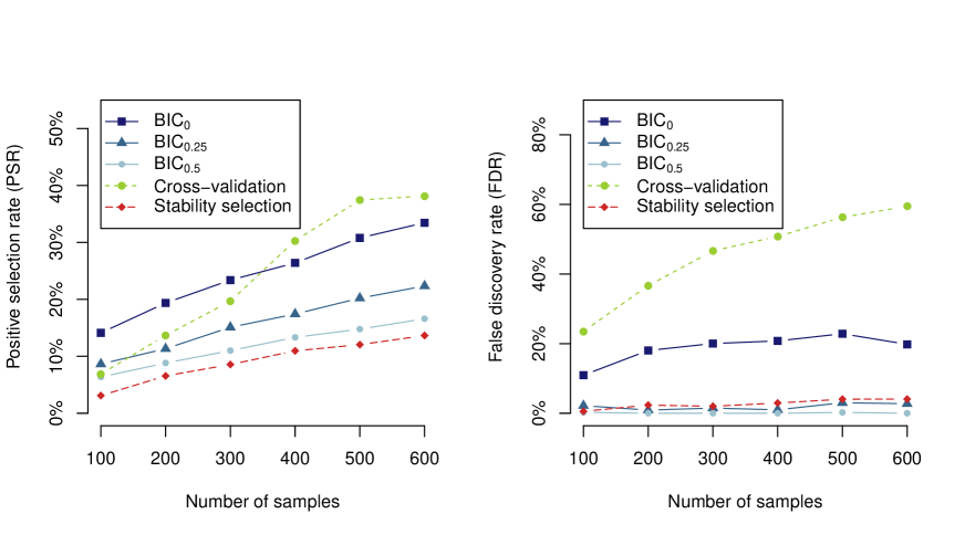
Figure 1. Results for the spam email detection experiment.

Comparing the three BICs to cross-validation, we observe that cross-validation can recover more true features (for larger values of $n$), but at an unacceptably large increase in the FDR. The original BIC performs better but still exhibits a high FDR. In contrast, the FDR of the EBIC with either $\gamma=0.25$ or $\gamma=0.5$ remains very low at all sample sizes; the associated PSR is smaller but increasing with the sample size. Stability selection performed similarly to the EBIC with $\gamma=0.5$ in this experiment, but with slightly lower PSR and slightly higher FDR. Overall, it seems that the EBIC with $\gamma=0.25$ performed best at the task of identifying the 57 true features, with a very low FDR and a moderately good PSR.

The rather low PSRs observed in the simulations are due in part to the fact that the 57 true features are not necessarily all strongly relevant to the response. To account for this in our evaluation of the five methods, we ran a logistic regression using the full data set (with a sample size of 4,601 emails) using the glm function in R, and extracted the p-values for each feature. For each method, using the models selected by the method over 100 repetitions of the experiment with $(n,p)=(600,57\cdot 24)$, we use Gaussian smoothing (scale: standard deviation = 0.1, on the p-value scale) to estimate, as a function of $t$, the probability that the method will select a true feature with p-value $t$. The estimated functions are plotted in Figure 2. (The rate of selection of false (permuted) features is not shown in this figure.) We see that the function estimates for cross-validation and the BICs each decay steadily with p-value, which seems desirable. In this experiment, stability selection appears to distinguish less clearly between highly and moderately relevant features, if we accept the p-values as a reasonable measure of relevance.

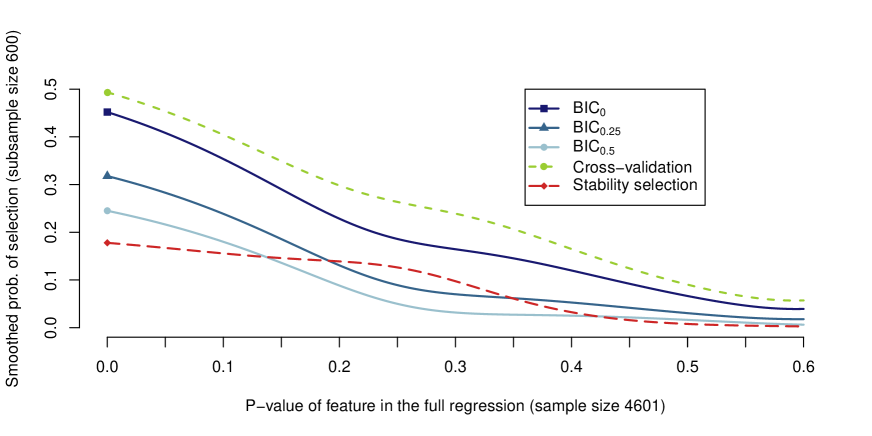
Figure 2. Smoothed probability of selecting a true feature, as a function of the p-value of that feature in the full regression.

5. Edge selection in sparse graphical models

In many applications, sparse graphical models are used to analyze data arising from multivariate observations with sparse dependency structure. In the setting we treat here, an undirected graph $G$ consists of a set of nodes $V$ representing the observed variables, and a set of undirected edges $E\in V\times V$ representing possible conditional dependencies between pairs of nodes. Specifically, if two of the variables do not have an edge between their corresponding nodes, then they are conditionally independent given all other observed variables. The problem of graphical model selection consists in selecting an appropriate set of edges to include in the graph that represents the dependency structure among the observed variables.

In Section 5.1, we introduce different approaches to this edge selection problem. In Sections 5.2 and 5.3, we discuss existing and new theoretical results for two commonly used classes of sparse graphical models.

5.1. Sparse graphical models

Suppose we observe $n$ independent and identically distributed random vectors in $\mathbb{R}^{p}$, denoted $X_{i\scriptscriptstyle\bullet}=(X_{i1},\dots,X_{ip})$, for $i=1,\dots,n$. For each graph $G$ on the set of nodes $V=\{1,\dots,p\}$, associate the model $\mathcal{M}_{G}$ comprising all distributions for which the conditional independence constraints implied by $G$ are satisfied. We are then interested in the recovery of the graph $G^{*}$ that encodes the dependency structure in the common true distribution of $X_{1\scriptscriptstyle\bullet},\dots,X_{n\scriptscriptstyle\bullet}$.

Since optimizing over the set of all (sparse) graphs is computationally infeasible, $\ell_{1}$-norm penalization methods have been considered. These ‘graphical Lasso’ procedures maximize the sum of the log-likelihood function and the absolute values of the relevant interaction parameters. As in the regression problem in (7), a tuning parameter $\rho$ is introduced to allow for the necessary trade-off between log-likelihood function and penalty term. This approach is the most tractable for the Gaussian case in which the penalty is the sum of the absolute values of the off-diagonal entries of the precision matrix $\Theta$ (Banerjee et al., 2008; Friedman et al., 2008). With the $\ell_{1}$-norm promoting sparsity in the estimate $\widehat{\Theta}^{\rho}$, a graph estimate $\widehat{G}^{\rho}_{\mathrm{glasso}}$ can be obtained by including an edge between nodes $j$ and $k$ whenever $\widehat{\Theta}^{\rho}_{jk}\neq 0$. Ravikumar et al. (2011) show that, under eigenvalue and irrepresentability assumptions on the true precision matrix $\Theta^{*}$, the estimate $\widehat{G}^{\rho}_{\mathrm{glasso}}$ is asymptotically consistent for a suitable sequence of values of $\rho$.

A similar approach is the neighborhood selection method of Meinshausen and Bühlmann (2006), which performs penalized regression for selecting each node’s neighborhood. Specifically, for each variable $j$, we optimize a penalized conditional likelihood function to find

$$\widehat{\beta}_{j}^{\rho}=\arg\min{}_{\beta_{j}}\Big{\{}-\sum_{i}\log\mathbb{P}(X_{ij}|\{X_{ik}:k\neq j\},\beta_{j})+\rho\|\beta_{j}\|_{1}\Big{\}}\;.$$

We then define the graph estimate $\widehat{G}^{\rho}_{\mathrm{neighbor}}$ to have an edge between nodes $j$ and $k$ whenever $\widehat{\beta}^{\rho}_{jk}$ and $\widehat{\beta}^{\rho}_{kj}$ are both nonzero (the and rule), or whenever either $\widehat{\beta}^{\rho}_{jk}$ or $\widehat{\beta}^{\rho}_{kj}$ is nonzero (the or rule). This method inherits asymptotic consistency properties from results for the individual regressions.

Both of the above methods require choosing the tuning parameter $\rho$. Similarly, greedy search over all graphs requires a choice of a sparsity bound $q$, or alternately, a stopping criterion to indicate when enough edges have been added. In each case, we can rephrase the tuning problem as the question of selecting a model from a small list of candidate graphs $G_{1},\dots,G_{m}$, of various sparsity levels.

We can use cross-validation to select a model from this list, but there are two disadvantages. First, $K$-fold cross-validation can be computationally expensive due to the process of fitting models to $K$ different parts of the data. More importantly, from the point of view of graph recovery, cross-validation tends to choose overly large models leading to selection of many false positive edges, in the high-dimensional setting when $p\gg n$; compare Foygel and Drton (2010). As for regression, we can alternatively use stability selection (Meinshausen and Bühlmann, 2010), where we search for edges that are stable across sparse models fitted to subsamples of the data using graphical Lasso or neighborhood selection; see also Liu et al. (2010). This method has been shown to be asymptotically consistent in a range of settings. However, it again requires refitting the model many times for different subsamples. Finally, as a third approach, we may apply information criteria, and we now turn to two specific settings where the extended BIC yields a computationally inexpensive and asymptotically consistent procedure for edge selection.

5.2. Gaussian graphical models

Suppose the i.i.d. observations $X_{1\scriptscriptstyle\bullet},\dots,X_{p\scriptscriptstyle\bullet}$ are multivariate normal with precision (or inverse covariance) matrix $\Theta$. Then it is well known that $X_{1j}$ and $X_{1k}$ are conditionally independent given the remaining variables $\{X_{l}:l\neq j,k\}$ if and only if $\Theta_{jk}=0$. The Gaussian graphical model $\mathcal{M}_{G}$ associated with an undirected graph $G$ on nodes $V=\{1,\dots,p\}$ is the set of all multivariate normal distributions with $\Theta_{jk}=0$ when $j$ and $k$ are two distinct non-adjacent nodes in $G$.

Prior work proposes the use of the extended BIC for sparse Gaussian graphical model selection (Foygel and Drton, 2010; Gao et al., 2011). Accounting for a matrix parameter, the EBIC is defined as

$$\mathrm{BIC}_{\gamma}(G)=-2\ell_{[n]}(\widehat{\Theta}_{G})+|G|\cdot\log(n)+4|G|\gamma\cdot\log(p),$$

where $\ell_{[n]}(\widehat{\Theta}_{G})$ denotes the maximized log-likelihood function for the set of $n$ observations, and $|G|$ is the number of edges in the graph. Since each model is only fitted once (to the full data set), this method carries relatively low computational cost, while enjoying consistency properties. We now state a version of the main theorem from Foygel and Drton (2010), which gives conditions under which minimization of the EBIC leads to selection of the smallest true model $G^{*}$ when applied to any list of sparse decomposable graphs containing $G^{*}$; for a definition of decomposable graphs we refer the reader to Lauritzen (1996).

Theorem 3.

Suppose that the true graph $G^{*}$ is decomposable with $|G^{*}|\leq q$, and that the true precision matrix $\Theta^{*}\in\mathcal{M}_{G^{*}}$ has bounded condition number and minimum nonzero value $\theta_{0}$ bounded away from zero. Suppose that $p\propto n^{\kappa}$ for some $\kappa<1$, and that the true neighborhood size is bounded for each node. Fix any $\gamma>1-\frac{1}{4\kappa}$. Then with probability tending to one as $n\rightarrow\infty$,

$$\mathrm{BIC}_{\gamma}(G^{*})<\min\left\{\mathrm{BIC}_{\gamma}(G)\ :\ \text{$G$ is decomposable with $|G|\leq q$}\right\}.$$

Together with consistency results on the graphical Lasso and on neighborhood selection, this result implies that combining EBIC and either graphical Lasso or neighborhood selection gives a consistent method for edge selection under the assumptions stated. While our proof of the theorem relies on exact distribution theory applicable to decomposable graphs, we conjecture that the stated result holds without the restriction to decomposable graphs.

Gao et al. (2011) propose EBIC-based tuning of the so-called SCAD penalization method for graphical model selection and give a consistency result taylored to this method. The version of the EBIC studied by these authors has the maximum likelihood estimator replaced by the SCAD estimator, and the model search is restricted to a subset of the SCAD regularization path. No decomposability assumptions were needed by Gao et al. (2011).

5.3. Ising models

In the setting of binary observations $X_{1\scriptscriptstyle\bullet},\dots,X_{n\scriptscriptstyle\bullet}\in\{0,1\}^{p}$, the Ising model consists of probability mass functions of the form

(8) $$\mathbb{P}\big{(}(X_{11},\dots,X_{1p})=(x_{1},\dots,x_{p})\big{)}\propto\exp\bigg{\{}\sum_{j}\zeta_{j}x_{j}+\tfrac{1}{2}\sum_{j\neq k}\Theta_{jk}x_{j}x_{k}\bigg{\}}\;,$$

where $\zeta\in\mathbb{R}^{p}$ is any vector, and for identifiability we constrain $\Theta\in\mathbb{R}^{p\times p}$ to be a symmetric matrix with zero diagonal. This model originated in physics to model states of particles, where informally we have $\Theta_{jk}>0$ if particles $j$ and $k$ prefer to be in the same state, and $\Theta_{jk}<0$ if particles $j$ and $k$ prefer to be in different states. For background and applications, compare e.g. Kindermann and Snell (1980).

In the Ising model, the conditional distribution of $X_{1j}$ given $\{X_{1k}:k\neq j\}$ comes from the logistic model—from (8), we obtain

$$\mathbb{P}\big{(}X_{1j}=x_{j}|\{X_{1k}=x_{k}:k\neq j\}\big{)}\propto\exp\bigg{\{}\bigg{(}\zeta_{j}+\sum_{k\neq j}\Theta_{jk}x_{k}\bigg{)}x_{j}\bigg{\}}\;,$$

and therefore the log-odds are

$$\log\left(\frac{\mathbb{P}\big{(}X_{1j}=1|\{X_{1k}:k\neq j\}\big{)}}{\mathbb{P}\big{(}X_{1j}=0|\{X_{1k}:k\neq j\}\big{)}}\right)=\zeta_{j}+\sum_{k\neq j}\Theta_{jk}X_{1k}\;.$$

To recover the true graph $G^{*}$ that describes the dependencies among the variables (or equivalently, the sparsity pattern in the true matrix $\Theta^{*}$), we can thus use neighborhood selection with the logistic Lasso, which finds

$$\widehat{\beta}_{j}^{\rho} =\arg\min{}_{\beta_{j}}\bigg{\{}-\sum_{i}\log\mathbb{P}\big{(}X_{ij}|\{X_{ik}:k\neq j\},\beta_{j}\big{)}+\rho\|\beta_{j}\|_{1}\bigg{\}}$$

$$=\arg\min{}_{\beta_{j}}\bigg{\{}-X_{ij}\cdot\bigg{(}\beta_{j0}+\sum_{k\neq j}X_{ik}\beta_{jk}\bigg{)}+\log\bigg{(}1+\exp\Big{\{}\beta_{j0}+\sum_{k\neq j}X_{ik}\beta_{jk}\Big{\}}\bigg{)}+\rho\|\beta_{j}\|_{1}\bigg{\}}\;.$$

The resulting graph estimate $\widehat{G}^{\rho}$ has an edge between nodes $j$ and $k$ based on the values of $\widehat{\beta}^{\rho}_{jk}$ and $\widehat{\beta}^{\rho}_{kj}$, using either an and or an or rule; compare also Höfling and Tibshirani (2009).

Tuning the parameter $\rho$ can be done using the EBIC for logistic regression. Our results for consistency of the EBIC for logistic regression then imply consistency guarantees for neighborhood selection with EBIC tuning. We assume that the following conditions hold (for constants $q$ and $c$):

• The growth of $p$ is subexponential, that is, $\log(p)=\mathbf{o}(n)$, with $\kappa\coloneqq\lim\sup\log_{n}(p)\in[0,\infty]$.

• The true graph $G^{*}$ has degree bounded by $q$, that is, each node $j$ has a neighborhood of cardinality $\left|\{k:(j,k)\in G^{*}\}\right|\leq q$.

• The true parameters are bounded with $\max{}_{j}|\zeta^{*}_{j}|\leq c$ and $\max{}_{j,k}|\Theta^{*}_{jk}|\leq c$.

• The signal is bounded away from zero such that

  $$\sqrt{\frac{\log(np)}{n}}=\mathbf{o}\left(\min_{(j,k)\in G^{*}}|\Theta^{*}_{jk}|\right)\;.$$

The following theorem gives a precise statement of the consistency properties of the EBIC for edge selection in the Ising model.

Theorem 4.

Assume that conditions (C1)-(C4) hold. Let $X_{1\scriptscriptstyle\bullet},\dots,X_{n\scriptscriptstyle\bullet}\in\{0,1\}^{p}$ be i.i.d. draws from an Ising model with parameters $\zeta^{*}\in\mathbb{R}^{p}$ and $\Theta^{*}\in\mathbb{R}^{p\times p}$, where $\Theta^{*}$ is symmetric with zero diagonals. Let $G^{*}$ be the graph with edges indicating the nonzero entries of $\Theta^{*}$, and for each node $j$, let $\mathcal{S}^{*}_{j}$ denote its true neighborhood, that is, $\mathcal{S}_{j}=\{k\neq j:\Theta^{*}_{jk}\neq 0\}$. Choose three scalars $\alpha,\beta,\gamma$ to satisfy

$$\left\{\text{\begin{tabular}[]{ll}\rule{0.0pt}{11.19443pt}\rule[-5.16663pt]{0.0pt}{0.0pt}$\gamma>1-\tfrac{1}{2\kappa}+\beta+\tfrac{\alpha}{\kappa}$,&if $\kappa>0$,\\ \rule{0.0pt}{11.19443pt}\rule[-5.16663pt]{0.0pt}{0.0pt}$\alpha\in\left(0,\tfrac{1}{2}\right)$ and $\beta>0$,&if $\kappa=0$.\\ \end{tabular}}\right.$$

Then, for sufficiently large $n$, the event that the inequalities

$$\mathrm{BIC}_{\gamma}(\mathcal{S}^{*}_{j})<\min\left\{\mathrm{BIC}_{\gamma}(\mathcal{S}_{j}):\mathcal{S}_{j}\not\ni j,\ \mathcal{S}_{j}\neq\mathcal{S}_{j}^{*},\ |\mathcal{S}_{j}|\leq q\right\}-\log(p)\cdot\left(\gamma-\left(1-\frac{1}{2\kappa}+\beta+\frac{\alpha}{\kappa}\right)\right)$$

hold simultaneously for all $j$ has probability at least $1-n^{-\alpha}p^{-(\beta-1)}$. In particular, the EBIC is consistent for neighborhood selection (simultaneously for all nodes) in the Ising model, whenever $\gamma>2-\frac{1}{2\kappa}$.

5.4. Experiment for the Ising model

We compared the BIC, the EBIC with $\gamma=0.25$ and $\gamma=0.5$, 10-fold cross-validation, and stability selection as in Meinshausen and Bühlmann (2010) on the task of edge selection under an Ising model for precipitation data from weather stations across four states in the midwest region of the U.S.: Illinois, Indiana, Iowa, and Missouri. Performance is measured relative to the true geographical layout of the weather stations, which is “unknown” to the procedures we compare.

5.4.1. Data and methods for model selection

We used data from the United States Historical Climatology Network (Menne et al., 2011). The data consists of weather-related variables that were recorded on a daily basis. We specifically gathered the precipitation data, which gives the total amount of precipitation for each day. Trying to limit the effects of temporal dependencies between successive observations, we took data from the 1st and 16th of each month. These are then treated as independent. We removed weather stations where data availability was low and discarded observations with missing values for any of the remaining weather stations. A total of 278 days and 89 stations remained in the final data set. Next, we hypothesized a “true” graph by computing the Delaunay triangulation of these 89 weather stations, based on their geographic locations, using the delaunay command in MATLAB (2010). Figure 3 shows a map with the resulting undirected graph.

Figure 3. Delaunay triangulation for 89 weather stations in Illinois, Indiana, Iowa, and Missouri.

For each weather station $j$, we define binary variables $X_{ij}$ taking values 1 or 0 depending on whether or not there was a positive amount of rainfall at weather station $j$ on day $i$. For each one of the stations $j$, we then applied each of the five methods to perform a sparse logistic regression that has response vector $X_{\scriptscriptstyle\bullet j}$ and covariates $\{X_{\scriptscriptstyle\bullet k}:k\neq j\}$. Our method for selecting a neighborhood for weather station $j$, for each of the five methods, is identical to our methods for the regression experiment on email data (see Section 4.2.1). Finally, we combined each method with the or rule and with the and rule to produce a sparse graph, for a total of ten methods.

5.4.2. Results

To evaluate the methods, we first treat the graph obtained via the Delaunay triangulation as the “true” underlying graphical model. Table 3 shows the results for each method, stated in terms of positive selection rate (PSR) and false discovery rate (FDR), relative to the “true” Delaunay triangulation graph. These results are also displayed in Figure 4, while the graphs in Figure 5 show the recovered graphs for each of the methods, combined with the and or or rules.

Table 3. Positive selection rate and false discovery rate in the weather data experiment.

	or rule		and rule
	PSR	FDR	PSR	FDR
BIC0.0	50.99	47.13	36.36	30.83
BIC0.25	45.45	39.47	30.04	28.97
BIC0.5	42.29	33.95	23.32	26.25
Cross-validation	69.17	76.42	59.29	65.83
Stability selection	24.51	26.19	13.44	26.09

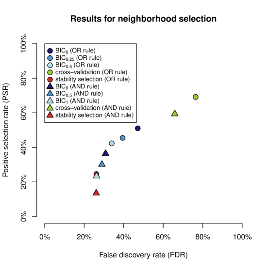
Figure 4. Performance of each method, under the or rule and the and rule, where the true graph is defined via the Delaunay triangulation.

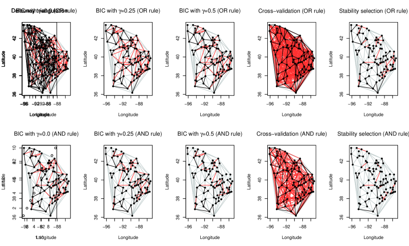
Figure 5. Graphs recovered under each method. (Black edges indicate true positives, red edges indicate false positives, and light gray edges indicate false negatives, i.e. true edges that were not recovered by the method, where the true graph is defined via the Delaunay triangulation.)

We see that cross-validation leads to a PSR that is somewhat higher than that of the other methods, under either an and or an or rule. However, this comes at a drastically higher FDR. For the EBIC, as we increase $\gamma$, we reduce the FDR at a cost of a lower PSR, as expected. Stability selection appears to be a more conservative method than $\mathrm{BIC}_{\gamma}$ for $\gamma=0.0,0.25,0.5$, with lower FDR and lower PSR, and was substantially more computationally expensive. While not shown, setting $\gamma=1.0$ with the EBIC yielded very similar results to stability selection, in this experiment.

The edges of the Delaunay triangulation likely capture the strongest dependencies, but it is reasonable to expect additional dependencies that are not captured by the edges in the triangulation. One way to compare the methods without referring to the Delaunay triangulation is to use the geographic distance between each pair of weather stations. For each method, we use Gaussian smoothing (scale: standard deviation = 10 miles) to estimate, as a function of $d$, the probability that the method will infer an edge between two nodes that are $d$ miles apart. The resulting functions are plotted in Figure 6, where we also show the same smoothed function calculation for the graph defined by the Delaunay triangulation.

We observe that the smoothed function for the cross-validation methods (under either the or or the and rule) does not decay to zero as distance increases. That is, in this experiment, the cross-validation methods tended to select some positive proportion of edges between nodes that are arbitrarily far apart, which is undesirable. To a lesser extent, the same problem occurs for the (original) BIC combined with the or rule. The other methods, in contrast, yield functions that do decay to zero as distance increases. We see also that for two nearby weather stations, the extended BIC with $\gamma=0.25$ or $\gamma=0.5$ combined with the or rule, are both significantly more likely to select an edge than the remaining methods, which are more conservative. Overall, the performance of the extended BIC compares favorably to the other methods, with a moderately good rate of edge selection for nearby weather stations, and with probability of edge selection decaying to zero when the distance between a pair of weather stations is large.

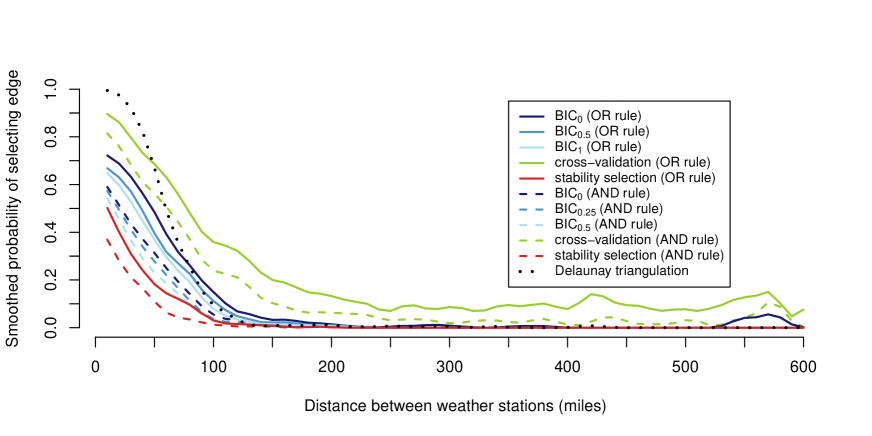
Figure 6. Smoothed probability of selecting edges as a function of distance, for each method under the or rule and the and rule.

6. Proof sketches for theorems

To prove our Theorems, we use Taylor series to approximate log-likelihood functions, and Laplace approximations to approximate integrated likelihoods. In Section 6.1 we introduce notation and state two technical lemmas bounding various quantities relating to the log-likelihood function. In Sections 6.2, 6.3, and 6.4 we outline the proofs of Theorems 1, 2, and 4, respectively. Full proofs are in the Appendix.

6.1. Preliminaries

Let $s_{[n]}(\phi)=\nabla\log L_{[n]}(\phi)\in\mathbb{R}^{p}$ be the gradient of the log likelihood (or score) function, and let $H_{[n]}(\phi)=-\nabla s_{[n]}(\phi)\in\mathbb{R}^{p\times p}$ be the Hessian. Write $s_{J}(\phi)$ and $H_{J}(\phi)$ to denote the sub-vector and sub-matrix, respectively, indexed by $j\in J$.

The following lemma gives bounds that will be important in the proofs of the Theorems.

Lemma 1.

Fix any $\alpha,\beta>0$. Assume (B1)-(B5) hold, and that either (A1) or (A2) holds. For sufficiently large $n$, with probability at least $1-n^{-\alpha}p^{-\beta}$ under (A1), or with probability at least $1-n^{-\alpha}p^{-\beta}-4K^{K+1}n^{-\frac{K-2\kappa}{2}}$ under (A2), the following statements are all true. The symbols $C_{1}$, $C_{2}$, $\lambda_{1}^{*}$, $\tau$, $R$, $\lambda_{1}$, $\lambda_{2}$, and $\lambda_{3}$ appearing in the statements represent constants that do not depend on $n$, $p$, or on the data, but generally are functions of other constants appearing in our assumptions.

• The gradient of the likelihood is bounded at the true parameter vector $\phi^{*}$:

  $$\left\|\left(H_{J}(\phi^{*})^{-\nicefrac{{1}}{{2}}}\right)s_{J}(\phi^{*})\right\|_{2}<\sqrt{2\left(1+\epsilon_{n}\right)\left|J\backslash J^{*}\right|\log\left(n^{\alpha}p^{1+\beta}\right)}\text{ for all $J\supsetneq J^{*}$ with $|J|\leq 2q$}\;,$$

  where $\epsilon_{n}=C_{1}\sqrt{\frac{\log\left(n^{\alpha}p^{1+\beta}\right)}{n}}+C_{2}\frac{1}{\log(n)}=\mathbf{o}(1)$.

• Likelihood is upper-bounded by a quadratic function:

  $$\log\left(\frac{L_{[n]}(\phi^{*}+\psi_{J})}{L_{[n]}(\phi^{*})}\right)\leq-\frac{\lambda_{1}^{*}n}{2}\|\psi_{J}\|_{2}\left(\min\{1,\|\psi_{J}\|_{2}\}-\tau\sqrt{\frac{\log\left(n^{\alpha}p^{1+\beta}\right)}{n}}\right)\text{ for all $|J|\leq 2q$, $\psi_{J}\in\mathbb{R}^{J}$}\;.$$

• For all sparse models, the MLE lies inside a compact set:

  $$\big{\|}\widehat{\phi}_{J}\big{\|}_{2}\leq R\text{ for all $|J|\leq 2q$}\;.$$

• The eigenvalues of the Hessian are bounded from above and below, and local changes in the Hessian are bounded from above, on the relevant compact set:

  $$\text{For all $|J|\leq 2q$, $\|\phi_{J}\|_{2}\leq R+1$, }\lambda_{1}\mathbf{I}_{J}\preceq\tfrac{1}{n}H_{J}(\phi_{J})\preceq\lambda_{2}\mathbf{I}_{J}\;,$$

  $$\text{and for all $\|\phi_{J}\|_{2},\|\phi^{\prime}_{J}\|_{2}\leq R+1$, }\tfrac{1}{n}\left(H_{J}(\phi_{J})-H_{J}(\phi^{\prime}_{J})\right)\preceq\|\phi_{J}-\phi^{\prime}_{J}\|_{2}\lambda_{3}\mathbf{I}_{J}\;.$$

We now state a second Lemma, which relates specifically to lower-bounding the eigenvalues of the Hessian, and may be of independent interest, as it holds under much weaker assumptions than those used in our other results.

Lemma 2.

Fix $J$ with $|J|=2q$, and radius $R>0$. Assume $\lambda_{\min}\left(\mathbb{E}\left[X_{1J}X_{1J}^{T}\right]\right)\geq a_{1}>0$ and $\sup_{j\in J}\mathbb{E}\left[\left|X_{1j}\right|^{4}\right]\leq m$. If $n$ is sufficiently large, then with probability at least $1-e^{-\left(150\cdot\left\lceil 80q^{2}ma_{1}^{-2}\right\rceil\right)^{-1}n}$, for all $\phi=\phi_{J}$ with $\|\phi\|_{2}\leq r$,

$$H_{J}(\phi)\succeq n\mathbf{I}_{J}\cdot\frac{a_{1}}{4}\inf\left\{\mathbf{b}^{\prime\prime}(\theta):|\theta|\leq 20q^{2}r\sqrt{m}\left\lceil 80q^{2}ma_{1}^{-2}\right\rceil\right\}\;.$$

6.2. Proof outline for Theorem 1

The key bound in the proof is showing that

$$\int_{\phi_{J}\in\mathbb{R}^{J}}L_{[n]}(\phi_{J})f_{J}(\phi_{J})\;d\phi_{J}=L_{[n]}(\widehat{\phi}_{J})f_{J}(\widehat{\phi}_{J})\cdot\left|H_{J}(\widehat{\phi}_{J})\right|^{-\nicefrac{{1}}{{2}}}(2\pi)^{\nicefrac{{|J|}}{{2}}}\cdot\left(1\pm C\sqrt{\frac{\log(np)}{n}}\right)\;,$$

for all $J$ with $|J|\leq q$. To this end, we calculate the marginal likelihood in each model $J$ by splitting the integration domain into three regions—a small neighborhood of the MLE called $\mathcal{N}_{1}$, a larger region $\mathcal{N}_{2}\backslash\mathcal{N}_{1}$ obtained from a larger neighborhood $\mathcal{N}_{2}$, and the remainder of the space, given by $\mathbb{R}^{J}\backslash\mathcal{N}_{2}$.

Fix any model $J$ with $|J|\leq q$, and let $\widehat{\phi}_{J}$ be the MLE. Define the neighborhoods

$$\mathcal{N}_{1}\coloneqq\left\{\phi:\left\|H_{J}(\widehat{\phi}_{J})^{\nicefrac{{1}}{{2}}}(\phi_{J}-\widehat{\phi}_{J})\right\|_{2}\leq\sqrt{4\log(np)}\right\}\;,$$

$$\mathcal{N}_{2}\coloneqq\left\{\phi:\left\|H_{J}(\widehat{\phi}_{J})^{\nicefrac{{1}}{{2}}}(\phi_{J}-\widehat{\phi}_{J})\right\|_{2}\leq\sqrt{\lambda_{1}n}\right\}\;.$$

Then the marginal likelihood is the sum of the three integrals

(Int1) $$\coloneqq\int_{\phi_{J}\in\mathcal{N}_{1}}L_{[n]}(\phi_{J})f_{J}(\phi_{J})\;d\phi_{J}\,,$$

(Int2) $$\coloneqq\int_{\phi_{J}\in\mathcal{N}_{2}\backslash\mathcal{N}_{1}}L_{[n]}(\phi_{J})f_{J}(\phi_{J})\;d\phi_{J}\,,$$

(Int3) $$\coloneqq\int_{\phi_{J}\in\mathbb{R}^{J}\backslash\mathcal{N}_{2}}L_{[n]}(\phi_{J})f_{J}(\phi_{J})\;d\phi_{J}\,.$$

The bulk of the proof now consists of computing approximations to each of the three terms separately.

It is at first surprising that we split into three regions, rather than two, as is done in other work with ‘fixed $p$.’ The intuition for our split is as follows:

(Int1):

In the smallest region, $\mathcal{N}_{1}$, a quadratic approximation to the log-likelihood function is extremely accurate, and we can use it to prove the accuracy of the Laplace approximation for this part of the integral.

(Int2):

In the intermediate region $\mathcal{N}_{2}\backslash\mathcal{N}_{1}$, while the quadratic approximation to the log-likelihood function is no longer very accurate, we can still obtain a quadratic upper bound. Hence, the integrand behaves as $e^{-c\|\phi_{J}-\widehat{\phi}_{J}\|^{2}_{2}}$ for an appropriate constant $c$, meaning that we can use tail bounds for the $\chi^{2}$ distribution to prove that the contribution of this region is negligible.

(Int3):

Outside of $\mathcal{N}_{2}$, the quadratic approximation may no longer be accurate enough to use the same reasoning as for the intermediate region. However, due to convexity of log-likelihood function, the integrand is at most roughly $e^{-c^{\prime}\|\phi_{J}-\widehat{\phi}_{J}\|_{2}}$ for an appropriate constant $c^{\prime}$. (Note that the quantity in the exponent is no longer squared.) Therefore, we can use tail bounds for an exponential distribution, to show that the contribution from this third region is also negligible.

Exponential tail bounds are much weaker than those for the $\chi^{2}$ distribution, which explains why we separate the area outside of $\mathcal{N}_{1}$ into two regions—first, the intermediate region $\mathcal{N}_{2}\backslash\mathcal{N}_{1}$ which contains points that are relatively close to the MLE, for which we can apply strong tail bounds, and second, a region $\mathbb{R}^{J}\backslash\mathcal{N}_{2}$ where we can only apply weaker tail bounds, but where all points are rather far from the MLE.

6.3. Proof outline for Theorem 2

Lemma 1 deals with issues arising from random covariates. Given the results of Lemma 1, our proof of this theorem follows the same reasoning as that of Chen and Chen (2011). Only slight modifications are needed; we give the details in the appendix for completeness. The proof consists of two parts that separate the treatment of incorrect and of true models:

• An incorrect sparse model is a model $J$ with $J\not\supset J^{*}$. In such a model, the distance between $\widehat{\phi}_{J}$ and $\phi^{*}$ will be large enough such that the likelihood function of model $J$ achieves only low values. The model will thus not be chosen over the true model $J^{*}$. Specifically, the lower-bound on the signal in assumption (B5) ensures that the change in the EBIC when comparing model $J$ to model $J^{*}$, is at least on the order of $\log(np)$.

• A true model is a model $J$ with $J\supsetneq J^{*}$. In an overly-large true model, the achievable increase in likelihood due to the extra degrees of freedom will not be large enough to compensate for the increased model size, and so again $J$ will not be chosen over the smallest true model $J^{*}$. Specifically, the increase in the achievable log-likelihood will be bounded on the order of $|J\backslash J^{*}|\log(np)$, which will be outweighed by the additional penalty on the larger model $J$.

6.4. Proof outline for Theorem 4

Considering each of the $p$ regressions separately, we obtain consistency of the EBIC with probability at least $1-n^{-\alpha}p^{-\beta}$ via Theorem 2, as long as all the conditions (B1)-(B5) hold. Using our assumptions for this current theorem, all these conditions hold by assumption, except for the eigenvalue bounds on $\mathbb{E}\left[X_{1J}X_{1J}^{T}\right]$ for all $|J|\leq 2q$. We derive these bounds in the appendix, using properties of the logistic model combined with the conditions assumed to be true.

7. Conclusion

As discussed in detail in the introduction in Section 1, the results in this paper make a formal connection between Bayesian model determination and model search using recently-proposed extended Bayesian information criteria (EBIC). Our results pertain to sparse high-dimensional generalized linear models based on a one-dimensional univariate exponential family and with canonical link. Evidently, a number of generalizations would be of interest for future work.

Remaining in the univarate exponential family framework, regression under non-canonical link could be considered in a fashion similar to what we have done here. Very recently, a treatment of this problem in the vein of Chen and Chen (2011) has been undertaken by Luo and Chen (2011b). Another extension would be to allow for exponential families with more than one parameter in regression models. This would in particular recover results for linear regression with unknown variance as a special case.

A different paradigm would be the graphical model setting. As reviewed in Section 5.1, there is a version of the EBIC that enjoys consistency properties in the Gaussian case. However, it remains an open problem to establish a formal connection to fully Bayesian graph selection procedures. Moreover, we hope that the available consistency results can be strengthened to avoid, in particular, decomposability assumptions for the concerned graphs.

Appendix A Proof of Theorem 1

Theorem 1.

Assume that conditions (B1)-(B5) hold, and that either assumption (A1) or (A2) holds. Moreover, assume the following mild conditions on the family of priors $\left(f_{J}:J\subset[p],|J|\leq q\right)$, which require the existence of constants $0<F_{1},F_{2},F_{3}<\infty$ such that, uniformly for all $|J|\leq q$, we have

• an upper bound on the priors:

  $$\sup{}_{\phi_{J}}f_{J}(\phi_{J})\leq F_{1}<\infty,$$

• a lower bound on the priors over a compact set:

  $$\inf{}_{\|\phi_{J}\|_{2}\leq R+1}f_{J}(\phi_{J})\geq F_{2}>0,$$

  where $R$ is a function of the constants in assumptions (A1) or (A2) and (B1)-(B5), defined in the proofs,

• a Lipschitz property on the same compact set:

  $$\sup{}_{\|\phi_{J}\|_{2}\leq R+1}\left\|\nabla f_{J}(\phi_{J})\right\|_{2}\leq F_{3}<\infty.$$

Then there is a constant $C$, no larger than $4F_{3}F_{2}^{-1}\lambda_{1}^{-\nicefrac{{1}}{{2}}}+2q\lambda_{3}\lambda_{1}^{-\nicefrac{{3}}{{2}}}+2$, such that, for sufficiently large $n$, the event that

(9) $$\mathrm{Bayes}(J)=P(J)\cdot L_{[n]}(\widehat{\phi}_{J})f_{J}(\widehat{\phi}_{J})\cdot\left|H_{J}(\widehat{\phi}_{J})\right|^{-\nicefrac{{1}}{{2}}}(2\pi)^{\nicefrac{{|J|}}{{2}}}\cdot\left(1\pm C\sqrt{\frac{\log(np)}{n}}\right)$$

uniformly for all models $J$ with $|J|\leq q$ occurs with probability at least $1-(np)^{-1}$ under (A1), and with probability at least $1-(np)^{-1}-4K^{K+1}n^{-\frac{K-2\kappa}{2}}$ under (A2). In particular, for the (unnormalized) prior $P(J)={p\choose|J|}^{-\gamma}\cdot{\mathbbm{1}}\left\{{|J|\leq q}\right\}$, it holds that

(10) $$\left|\log\left(\mathrm{Bayes}_{\gamma}(J)\right)-\left(-\tfrac{1}{2}\mathrm{BIC}_{\gamma}(J)\right)\right|\leq C_{1}\;,$$

where $C_{1}$ is a constant no larger than $\tfrac{q}{2}\log(2\pi)+\gamma q\log(2q)+q\log\max\{\lambda_{1}^{-1},\lambda_{2}\}+\log\max\{F_{1},F_{2}^{-1}\}+1$.

Proof.

First, we show that the approximation (9) to the Bayesian marginal likelihood will imply the bound (10). We have

$$\log\left(\mathrm{Bayes}_{\gamma}(J)\right)=\log\left(P(J)\cdot L_{[n]}(\widehat{\phi}_{J})f_{J}(\widehat{\phi}_{J})\cdot\left|H_{J}(\widehat{\phi}_{J})\right|^{-\nicefrac{{1}}{{2}}}(2\pi)^{\nicefrac{{|J|}}{{2}}}\cdot\left(1\pm C\sqrt{\frac{\log(np)}{n}}\right)\right)$$

$$=-\gamma\log{p\choose|J|}+\log L_{[n]}(\widehat{\phi}_{J})+\log f_{J}(\widehat{\phi}_{J})-\tfrac{1}{2}\log\left|H_{J}(\widehat{\phi}_{J})\right|+\tfrac{|J|}{2}\log(2\pi)+\log\left(1\pm C\sqrt{\frac{\log(np)}{n}}\right)\;.$$

We now approximate some of the above terms. First, by definition of ${p\choose|J|}$, we have

$$|J|\log(p)\geq\log{p\choose|J|}\geq\log\left(\frac{(p-|J|)^{|J|}}{|J|^{|J|}}\right)\geq\log\left(\left(\frac{p}{2|J|}\right)^{|J|}\right)\geq|J|\log(p)-q\log(2q)\;.$$

Next, since $\lambda_{1}n\mathbf{I}_{J}\preceq H_{J}(\widehat{\phi}_{J})\preceq\lambda_{2}n\mathbf{I}_{J}$, we have

$$|J|\log(n)+|J|\log(\lambda_{1})=\log\left|\lambda_{1}n\mathbf{I}_{J}\right|\leq\log\left|H_{J}(\widehat{\phi}_{J})\right|\leq\log\left|\lambda_{2}n\mathbf{I}_{J}\right|=|J|\log(n)+|J|\log(\lambda_{2})\;.$$

Finally, $F_{2}\leq\log f_{J}(\widehat{\phi}_{J})\leq F_{1}$ by assumption, and for sufficiently large $n$, $C\sqrt{\frac{\log(np)}{n}}\leq\frac{1}{2}$. Combining all of the above, we get

$$\log\left(\mathrm{Bayes}_{\gamma}(J)\right)=\log L_{[n]}(\widehat{\phi}_{J})-\tfrac{|J|}{2}\log(n)-\gamma|J|\log(p)\pm C_{1}=-\tfrac{1}{2}\mathrm{BIC}_{\gamma}(J)\pm C_{1}\;,$$

where we define

$$C_{1}\coloneqq\tfrac{q}{2}\log(2\pi)+\gamma q\log(2q)+q\log\max\{\lambda_{1}^{-1},\lambda_{2}\}+\log\max\{F_{1},F_{2}^{-1}\}+1\;.$$

We next prove the approximation (9). We need to show that

$$\int_{\phi_{J}\in\mathbb{R}^{J}}L_{[n]}(\phi_{J})f_{J}(\phi_{J})\;d\phi_{J}=L_{[n]}(\widehat{\phi}_{J})f_{J}(\widehat{\phi}_{J})\cdot\left|H_{J}(\widehat{\phi}_{J})\right|^{-\nicefrac{{1}}{{2}}}(2\pi)^{\nicefrac{{|J|}}{{2}}}\cdot\left(1\pm C\sqrt{\frac{\log(np)}{n}}\right)\;,$$

for all $J$ with $|J|\leq q$.

To this end, for each model $J$, we split the integration domain into three regions—a small neighborhood of the MLE denoted by $\mathcal{N}_{1}$, a larger region $\mathcal{N}_{2}\backslash\mathcal{N}_{1}$ obtained by taking a larger neighborhood $\mathcal{N}_{2}$ and subtracting the first region, and the remainder of the space, given by $\mathbb{R}^{J}\backslash\mathcal{N}_{2}$.

Fix any model $J$ with $|J|\leq q$, and let $\widehat{\phi}_{J}$ be the MLE. Define the neighborhoods

$$\mathcal{N}_{1}\coloneqq\left\{\phi:\left\|H_{J}(\widehat{\phi}_{J})^{\nicefrac{{1}}{{2}}}(\phi_{J}-\widehat{\phi}_{J})\right\|_{2}\leq\sqrt{4\log(np)}\right\}\;,$$

$$\mathcal{N}_{2}\coloneqq\left\{\phi:\left\|H_{J}(\widehat{\phi}_{J})^{\nicefrac{{1}}{{2}}}(\phi_{J}-\widehat{\phi}_{J})\right\|_{2}\leq\sqrt{\lambda_{1}n}\right\}\;.$$

(We assume $n$ is large so that $\mathcal{N}_{1}\subset\mathcal{N}_{2}$.) We write

$$\int_{\phi_{J}\in\mathbb{R}^{J}}L_{[n]}(\phi_{J})f_{J}(\phi_{J})\;d\phi_{J}=$$

$$\hskip 28.45274pt\underbrace{\int_{\phi_{J}\in\mathcal{N}_{1}}L_{[n]}(\phi_{J})f_{J}(\phi_{J})\;d\phi_{J}}_{\text{(Int1)}}+\underbrace{\int_{\phi_{J}\in\mathcal{N}_{2}\backslash\mathcal{N}_{1}}L_{[n]}(\phi_{J})f_{J}(\phi_{J})\;d\phi_{J}}_{\text{(Int2)}}+\underbrace{\int_{\phi_{J}\in\mathbb{R}^{J}\backslash\mathcal{N}_{2}}L_{[n]}(\phi_{J})f_{J}(\phi_{J})\;d\phi_{J}}_{\text{(Int3)}}\;.$$

We now approximate to each of the three terms separately. First, by Lemma 1(iv), for a point $\phi_{J}\in\mathcal{N}_{2}$, $\|H_{J}(\widehat{\phi}_{J})^{\nicefrac{{1}}{{2}}}(\phi_{J}-\widehat{\phi}_{J})\|_{2}\leq\sqrt{\lambda_{1}n}$ implies $\|\phi_{J}-\widehat{\phi}_{J}\|_{2}\leq 1$. Therefore, integrals (Int1) and (Int2) are both computed in a neighborhood of radius $1$ around $\widehat{\phi}_{J}$. The main idea for the computations below is that the contributions of (Int2) and (Int3) are negligible, while the value of (Int1) can be very closely approximated by using the second-order Taylor series expansion to the likelihood.

Approximating (Int1). In a very small neighborhood around $\widehat{\phi}_{J}$, the quadratic approximation

$$\sum_{i}\ell_{i}(\phi_{J}) \approx\sum_{i}\ell_{i}(\widehat{\phi}_{J})+(\phi_{J}-\widehat{\phi}_{J})^{T}s_{J}(\widehat{\phi}_{J})-\frac{1}{2}(\phi_{J}-\widehat{\phi}_{J})^{T}H_{J}(\widehat{\phi}_{J})(\phi_{J}-\widehat{\phi}_{J})$$

$$=\sum_{i}\ell_{i}(\widehat{\phi}_{J})-\frac{1}{2}(\phi_{J}-\widehat{\phi}_{J})^{T}H_{J}(\widehat{\phi}_{J})(\phi_{J}-\widehat{\phi}_{J})$$

is very accurate, and we can therefore use a Laplace approximation to the integral in this small neighborhood, to obtain

(Int1) $$\approx\int_{\mathbb{R}^{J}}\exp\left\{\sum_{i}\ell_{i}(\widehat{\phi}_{J})-\frac{1}{2}(\phi_{J}-\widehat{\phi}_{J})^{T}H_{J}(\widehat{\phi}_{J})(\phi_{J}-\widehat{\phi}_{J})\right\}f_{J}(\widehat{\phi}_{J})\;d\phi_{J}$$

$$={(2\pi)^{\nicefrac{{|J|}}{{2}}}f_{J}(\widehat{\phi}_{J})}{\left|H_{J}(\widehat{\phi}_{J})\right|^{-\nicefrac{{1}}{{2}}}}\exp\left\{\sum_{i}\ell_{i}(\widehat{\phi}_{J})\right\}\;.$$

To make this approximation rigorous, we begin by giving precise bounds on the approximation to the likelihood in a neighborhood of $\widehat{\phi}_{J}$. By Lemma 1(iv), for any $\phi_{J}$ with $\|\phi_{J}-\widehat{\phi}_{J}\|_{2}\leq 1$, for some $t\in[0,1]$, we have

$$\sum_{i}\left(\ell_{i}(\phi_{J})-\ell_{i}(\widehat{\phi}_{J})\right) =\psi_{J}^{T}s_{J}(\widehat{\phi}_{J})-\frac{1}{2}(\phi_{J}-\widehat{\phi}_{J})^{T}H_{J}(\widehat{\phi}_{J}+t(\phi_{J}-\widehat{\phi}_{J}))(\phi_{J}-\widehat{\phi}_{J})$$

$$=-\frac{1}{2}(\phi_{J}-\widehat{\phi}_{J})^{T}H_{J}(\widehat{\phi}_{J}+t(\phi_{J}-\widehat{\phi}_{J}))(\phi_{J}-\widehat{\phi}_{J})$$

$$=-\frac{1}{2}(\phi_{J}-\widehat{\phi}_{J})^{T}H_{J}(\widehat{\phi}_{J})(\phi_{J}-\widehat{\phi}_{J})\pm\frac{1}{2}\|\phi_{J}-\widehat{\phi}_{J}\|^{2}_{2}\left\|H_{J}(\widehat{\phi}_{J}+t(\phi_{J}-\widehat{\phi}_{J}))-H_{J}(\widehat{\phi}_{J})\right\|_{\mathrm{sp}}$$

(11) $$=-\frac{1}{2}(\phi_{J}-\widehat{\phi}_{J})^{T}H_{J}(\widehat{\phi}_{J})(\phi_{J}-\widehat{\phi}_{J})\pm\frac{1}{2}\|\phi_{J}-\widehat{\phi}_{J}\|^{3}_{2}n\lambda_{3}\;.$$

(Here $\|M\|_{\mathrm{sp}}$ denotes the spectral norm of the matrix $M$.) Recall that for all $\phi_{J}\in\mathcal{N}_{1}\subset\mathcal{N}_{2}$, we have $\|\phi_{J}-\widehat{\phi}_{J}\|_{2}\leq 1$. Applying the approximation (11) for all $\phi_{J}\in\mathcal{N}_{1}$, we claim that

$$\text{(Int1)}=(2\pi)^{\nicefrac{{|J|}}{{2}}}f_{J}(\widehat{\phi}_{J})\left|H_{J}(\widehat{\phi}_{J})\right|^{-\nicefrac{{1}}{{2}}}\exp\left\{\sum_{i}\ell_{i}(\widehat{\phi}_{J})\right\}\cdot\left(1\pm\left(4F_{3}F_{2}^{-1}\lambda_{1}^{-\nicefrac{{1}}{{2}}}+2q\lambda_{3}\lambda_{1}^{-\nicefrac{{3}}{{2}}}+1\right)\cdot\sqrt{\frac{\log(np)}{n}}\right)\;.$$

We will now prove this bound.

Applying Lemma 1(iii), $\|\phi_{J}\|_{2}\leq\|\widehat{\phi}_{J}\|_{2}+\|\phi_{J}-\widehat{\phi}_{J}\|_{2}\leq R+1$. By our assumptions on $f_{J}$ on the ball of radius $R+1$ at zero,

$$\left\|\frac{\partial}{\partial\phi_{J}}\log f_{J}(\phi_{J})\right\|_{2}=\left\|\frac{\nabla f_{J}(\phi_{J})}{f_{J}(\phi_{J})}\right\|_{2}\leq F_{3}F_{2}^{-1}\;.$$

Next, since by Lemma 1(iv) we know that $H_{J}(\widehat{\phi}_{J})\succeq\lambda_{1}n\mathbf{I}_{J}$, we apply the definition of $\mathcal{N}_{1}$ to obtain

$$\|\phi_{J}-\widehat{\phi}_{J}\|^{3}_{2}n\lambda_{3}\leq\sqrt{\frac{4\log(np)}{\lambda_{1}n}}\cdot\|\phi_{J}-\widehat{\phi}_{J}\|^{2}_{2}\leq\sqrt{\frac{4\log(np)}{\lambda_{1}n}}\cdot(\phi_{J}-\widehat{\phi}_{J})^{T}H_{J}(\widehat{\phi}_{J})(\phi_{J}-\widehat{\phi}_{J})\cdot(\lambda_{1}n)^{-1}\;.$$

Applying the three above bounds, we obtain an upper bound on (Int1):

$$\text{(Int1)}=\int_{\mathcal{N}_{1}}\exp\left\{\sum_{i}\ell_{i}(\phi_{J})\right\}f_{J}(\phi_{J})\;d\phi_{J}$$

$$=\exp\left\{\sum_{i}\ell_{i}(\widehat{\phi}_{J})\right\}\int_{\mathcal{N}_{1}}\exp\left\{-\frac{1}{2}(\phi_{J}-\widehat{\phi}_{J})^{T}H_{J}(\widehat{\phi}_{J})(\phi_{J}-\widehat{\phi}_{J})\pm\frac{1}{2}\|\phi_{J}-\widehat{\phi}_{J}\|^{3}_{2}n\lambda_{3}\right\}f_{J}(\phi_{J})\;d\phi_{J}$$

$$\leq\exp\left\{\sum_{i}\ell_{i}(\widehat{\phi}_{J})\right\}\int_{\mathcal{N}_{1}}\exp\left\{-\frac{1}{2}(\phi_{J}-\widehat{\phi}_{J})^{T}H_{J}(\widehat{\phi}_{J})(\phi_{J}-\widehat{\phi}_{J})\left(1-\sqrt{\frac{4\lambda_{3}^{2}\log(np)}{\lambda_{1}^{3}n}}\right)\right\}f_{J}(\phi_{J})\;d\phi_{J}$$

$$\leq\exp\left\{\sum_{i}\ell_{i}(\widehat{\phi}_{J})+\log f_{J}(\widehat{\phi}_{J})+\sqrt{\frac{4\log(np)}{\lambda_{1}n}}F_{3}F_{2}^{-1}\right\}$$

$$\hskip 56.9055pt\times\int_{\mathcal{N}_{1}}\exp\left\{-\frac{1}{2}(\phi_{J}-\widehat{\phi}_{J})^{T}H_{J}(\widehat{\phi}_{J})(\phi_{J}-\widehat{\phi}_{J})\left(1-\sqrt{\frac{4\lambda_{3}^{2}\log(np)}{\lambda_{1}^{3}n}}\right)\right\}\;d\phi_{J}\;.$$

Changing variables to $$\xi=\left(1-\sqrt{\frac{4\lambda_{3}^{2}\log(np)}{\lambda_{1}^{3}n}}\right)^{-\nicefrac{{1}}{{2}}}H_{J}(\widehat{\phi}_{J})^{\nicefrac{{1}}{{2}}}(\phi_{J}-\widehat{\phi}_{J})$$, the upper bound becomes

$$\exp\left\{\sum_{i}\ell_{i}(\widehat{\phi}_{J})+\log f_{J}(\widehat{\phi}_{J})+\sqrt{\frac{4\log(np)}{\lambda_{1}n}}F_{3}F_{2}^{-1}\right\}\cdot\left|H_{J}(\widehat{\phi}_{J})\right|^{-\nicefrac{{1}}{{2}}}\left(1-\sqrt{\frac{4\lambda_{3}^{2}\log(np)}{\lambda_{1}^{3}n}}\right)^{-\nicefrac{{|J|}}{{2}}}$$

$$\hskip 56.9055pt\times\int_{\left\|\xi\right\|_{2}\leq\left(1-\sqrt{\frac{4\lambda_{3}^{2}\log(np)}{\lambda_{1}^{3}n}}\right)^{-\nicefrac{{1}}{{2}}}\sqrt{4\log(np)}}\;\exp\left\{-\frac{1}{2}\|\xi\|^{2}_{2}\right\}\;d\xi$$

$$\leq\exp\left\{\sum_{i}\ell_{i}(\widehat{\phi}_{J})+\log f_{J}(\widehat{\phi}_{J})+\sqrt{\frac{4\log(np)}{\lambda_{1}n}}F_{3}F_{2}^{-1}\right\}\cdot\left|H_{J}(\widehat{\phi}_{J})\right|^{-\nicefrac{{1}}{{2}}}\left(1-\sqrt{\frac{4\lambda_{3}^{2}\log(np)}{\lambda_{1}^{3}n}}\right)^{-\nicefrac{{|J|}}{{2}}}(2\pi)^{\nicefrac{{|J|}}{{2}}}$$

$$\hskip 56.9055pt\times\int_{\xi\in\mathbb{R}^{J}}(2\pi)^{-\nicefrac{{|J|}}{{2}}}\exp\left\{-\frac{1}{2}\|\xi\|^{2}_{2}\right\}\;d\xi$$

$$=\exp\left\{\sum_{i}\ell_{i}(\widehat{\phi}_{J})+\log f_{J}(\widehat{\phi}_{J})+\sqrt{\frac{4\log(np)}{\lambda_{1}n}}F_{3}F_{2}^{-1}\right\}\cdot\left|H_{J}(\widehat{\phi}_{J})\right|^{-\nicefrac{{1}}{{2}}}\left(1-\sqrt{\frac{4\lambda_{3}^{2}\log(np)}{\lambda_{1}^{3}n}}\right)^{-\nicefrac{{|J|}}{{2}}}(2\pi)^{\nicefrac{{|J|}}{{2}}}\;.$$

We similarly obtain a lower bound:

$$\text{(Int1)}=\int_{\mathcal{N}_{1}}\exp\left\{\sum_{i}\ell_{i}(\phi_{J})\right\}f_{J}(\phi_{J})\;d\phi_{J}$$

$$=\exp\left\{\sum_{i}\ell_{i}(\widehat{\phi}_{J})\right\}\int_{\mathcal{N}_{1}}\exp\left\{-\frac{1}{2}(\phi_{J}-\widehat{\phi}_{J})^{T}H_{J}(\widehat{\phi}_{J})(\phi_{J}-\widehat{\phi}_{J})\pm\frac{1}{2}\|\phi_{J}-\widehat{\phi}_{J}\|^{3}_{2}n\lambda_{3}\right\}f_{J}(\phi_{J})\;d\phi_{J}$$

$$\geq\exp\left\{\sum_{i}\ell_{i}(\widehat{\phi}_{J})\right\}\int_{\mathcal{N}_{1}}\exp\left\{-\frac{1}{2}(\phi_{J}-\widehat{\phi}_{J})^{T}H_{J}(\widehat{\phi}_{J})(\phi_{J}-\widehat{\phi}_{J})\left(1+\sqrt{\frac{4\lambda_{3}^{2}\log(np)}{\lambda_{1}^{3}n}}\right)\right\}f_{J}(\phi_{J})\;d\phi_{J}$$

$$\geq\exp\left\{\sum_{i}\ell_{i}(\widehat{\phi}_{J})+\log f_{J}(\widehat{\phi}_{J})-\sqrt{\frac{4\log(np)}{\lambda_{1}n}}F_{3}F_{2}^{-1}\right\}$$

$$\hskip 56.9055pt\times\int_{\mathcal{N}_{1}}\exp\left\{-\frac{1}{2}(\phi_{J}-\widehat{\phi}_{J})^{T}H_{J}(\widehat{\phi}_{J})(\phi_{J}-\widehat{\phi}_{J})\left(1+\sqrt{\frac{4\lambda_{3}^{2}\log(np)}{\lambda_{1}^{3}n}}\right)\right\}\;d\phi_{J}\;.$$

Changing variables to $$\xi=\left(1+\sqrt{\frac{4\lambda_{3}^{2}\log(np)}{\lambda_{1}^{3}n}}\right)^{-\nicefrac{{1}}{{2}}}H_{J}(\widehat{\phi}_{J})^{\nicefrac{{1}}{{2}}}(\phi_{J}-\widehat{\phi}_{J})$$, the lower bound becomes

$$\exp\left\{\sum_{i}\ell_{i}(\widehat{\phi}_{J})+\log f_{J}(\widehat{\phi}_{J})-\sqrt{\frac{4\log(np)}{\lambda_{1}n}}F_{3}F_{2}^{-1}\right\}\cdot\left|H_{J}(\widehat{\phi}_{J})\right|^{-\nicefrac{{1}}{{2}}}\left(1+\sqrt{\frac{4\lambda_{3}^{2}\log(np)}{\lambda_{1}^{3}n}}\right)^{-\nicefrac{{|J|}}{{2}}}(2\pi)^{\nicefrac{{|J|}}{{2}}}$$

$$\hskip 56.9055pt\times\int_{\left\|\xi\right\|_{2}\leq\left(1+\sqrt{\frac{4\lambda_{3}^{2}\log(np)}{\lambda_{1}^{3}n}}\right)^{-\nicefrac{{1}}{{2}}}\sqrt{4\log(np)}}(2\pi)^{-\nicefrac{{|J|}}{{2}}}\exp\left\{-\frac{1}{2}\|\xi\|^{2}_{2}\right\}\;d\phi_{J}$$

$$\geq\exp\left\{\sum_{i}\ell_{i}(\widehat{\phi}_{J})+\log f_{J}(\widehat{\phi}_{J})-\sqrt{\frac{4\log(np)}{\lambda_{1}n}}F_{3}F_{2}^{-1}\right\}\cdot\left|H_{J}(\widehat{\phi}_{J})\right|^{-\nicefrac{{1}}{{2}}}\left(1+\sqrt{\frac{4\lambda_{3}^{2}\log(np)}{\lambda_{1}^{3}n}}\right)^{-\nicefrac{{|J|}}{{2}}}(2\pi)^{\nicefrac{{|J|}}{{2}}}$$

$$\hskip 56.9055pt\times\mathbb{P}\left\{\chi^{2}_{|J|}\leq 2\log(np)\right\}$$

$$\geq\exp\left\{\sum_{i}\ell_{i}(\widehat{\phi}_{J})+\log f_{J}(\widehat{\phi}_{J})-\sqrt{\frac{4\log(np)}{\lambda_{1}n}}F_{3}F_{2}^{-1}\right\}\cdot\left|H_{J}(\widehat{\phi}_{J})\right|^{-\nicefrac{{1}}{{2}}}\left(1+\sqrt{\frac{4\lambda_{3}^{2}\log(np)}{\lambda_{1}^{3}n}}\right)^{-\nicefrac{{|J|}}{{2}}}(2\pi)^{\nicefrac{{|J|}}{{2}}}$$

$$\hskip 56.9055pt\times\left(1-e^{-\log(np)/2}\right)\;,$$

for sufficiently large $n$.

Combining the upper and lower bounds, we therefore have

$$\text{(Int1)}=\exp\left\{\sum_{i}\ell_{i}(\widehat{\phi}_{J})+\log f_{J}(\widehat{\phi}_{J})+\sqrt{\frac{4\log(np)}{\lambda_{1}n}}\frac{F_{3}}{F_{2}}\right\}$$

$$\hskip 108.405pt\cdot\left|H_{J}(\widehat{\phi}_{J})\right|^{-\nicefrac{{1}}{{2}}}\left(1-\sqrt{\frac{4\lambda_{3}^{2}\log(np)}{\lambda_{1}^{3}n}}\right)^{-\nicefrac{{|J|}}{{2}}}(2\pi)^{\nicefrac{{|J|}}{{2}}}\cdot(1-c)\;,$$

for some $c$ satisfying $0\leq c\leq e^{-\log(np)/2}$. Since $\log(np)=\mathbf{o}(n)$, we can thus write

$$\text{(Int1)}=(2\pi)^{\nicefrac{{|J|}}{{2}}}f_{J}(\widehat{\phi}_{J})\left|H_{J}(\widehat{\phi}_{J})\right|^{-\nicefrac{{1}}{{2}}}\exp\left\{\sum_{i}\ell_{i}(\widehat{\phi}_{J})\right\}\cdot\left(1\pm\left(4F_{3}F_{2}^{-1}\lambda_{1}^{-\nicefrac{{1}}{{2}}}+2q\lambda_{3}\lambda_{1}^{-\nicefrac{{3}}{{2}}}+1\right)\cdot\sqrt{\frac{\log(np)}{n}}\right)\;.$$

Bounding (Int2). For $\|\phi_{J}-\widehat{\phi}_{J}\|_{2}\leq 1$, we can apply Lemma 1(iii) and (iv) to see that $H_{J}(\phi_{J})\succeq\lambda_{1}n\mathbf{I}_{J}\succeq\lambda_{1}\lambda_{2}^{-1}H_{J}(\widehat{\phi}_{J})$. Therefore, by the Taylor series approximation, for $\|\phi_{J}-\widehat{\phi}_{J}\|_{2}\leq 1$, since $s_{J}(\widehat{\phi}_{J})=0$, we have

(12) $$\sum_{i}\ell_{i}(\phi_{J})\leq\sum_{i}\ell_{i}(\widehat{\phi}_{J})-\frac{\lambda_{1}\lambda_{2}^{-1}}{2}(\phi_{J}-\widehat{\phi}_{J})^{T}H_{J}(\widehat{\phi}_{J})(\phi_{J}-\widehat{\phi}_{J})\;,$$

and so

(Int2) $$=\int_{\sqrt{4\log(np)}<\left\|H_{J}(\widehat{\phi}_{J})^{\nicefrac{{1}}{{2}}}(\phi_{J}-\widehat{\phi}_{J})\right\|_{2}\leq\sqrt{\lambda_{1}n}}\exp\left\{\sum_{i}\ell_{i}(\phi_{J})\right\}f_{J}(\phi_{J})\;d\phi_{J}$$

$$\leq F_{1}\int_{\sqrt{4\log(np)}<\left\|H_{J}(\widehat{\phi}_{J})^{\nicefrac{{1}}{{2}}}(\phi_{J}-\widehat{\phi}_{J})\right\|_{2}}\exp\left\{\sum_{i}\ell_{i}(\widehat{\phi}_{J})-\frac{\lambda_{1}\lambda_{2}^{-1}}{2}(\phi_{J}-\widehat{\phi}_{J})^{T}H_{J}(\widehat{\phi}_{J})(\phi_{J}-\widehat{\phi}_{J})\right\}\;d\phi_{J}$$

$$=F_{1}\exp\left\{\sum_{i}\ell_{i}(\widehat{\phi}_{J})\right\}\left|H_{J}(\widehat{\phi}_{J})\right|^{-\nicefrac{{1}}{{2}}}(\lambda_{2}\lambda_{1}^{-1})^{\nicefrac{{|J|}}{{2}}}\int_{\|\xi\|^{2}_{2}>{{2\log(np)}}}\exp\left\{-\frac{1}{2}\|\xi\|^{2}_{2}\right\}\;d\xi$$

$$=F_{1}\exp\left\{\sum_{i}\ell_{i}(\widehat{\phi}_{J})\right\}\left|H_{J}(\widehat{\phi}_{J})\right|^{-\nicefrac{{1}}{{2}}}(\lambda_{2}\lambda_{1}^{-1})^{\nicefrac{{|J|}}{{2}}}\cdot(2\pi)^{\nicefrac{{|J|}}{{2}}}\mathbb{P}\left\{\chi^{2}_{|J|}>{{2\log(np)}}\right\}$$

$$\leq F_{1}\exp\left\{\sum_{i}\ell_{i}(\widehat{\phi}_{J})\right\}\left|H_{J}(\widehat{\phi}_{J})\right|^{-\nicefrac{{1}}{{2}}}(\lambda_{2}\lambda_{1}^{-1})^{\nicefrac{{|J|}}{{2}}}\cdot(2\pi)^{\nicefrac{{|J|}}{{2}}}\cdot e^{-\log(np)/2}\;,$$

by the chi-square tail bounds derived by Cai (2002).

Bounding (Int3). For all $\phi_{J}$ such that $\left\|H_{J}(\widehat{\phi}_{J})^{\nicefrac{{1}}{{2}}}(\phi_{J}-\widehat{\phi}_{J})\right\|_{2}=\sqrt{\lambda_{1}n}$, by (12), we know that

$$\sum_{i}\ell_{i}(\phi_{J})-\sum_{i}\ell_{i}(\widehat{\phi}_{J}) \leq-\frac{\lambda_{1}\lambda_{2}^{-1}}{2}(\phi_{J}-\widehat{\phi}_{J})^{T}H_{J}(\widehat{\phi}_{J})(\phi_{J}-\widehat{\phi}_{J})$$

$$=-\frac{\lambda_{1}\lambda_{2}^{-1}\cdot\sqrt{\lambda_{1}n}}{2}\left\|H_{J}(\widehat{\phi}_{J})^{\nicefrac{{1}}{{2}}}(\phi_{J}-\widehat{\phi}_{J})\right\|_{2}\;,$$

and so by convexity of likelihood, for all $\phi_{J}$ such that $\left\|H_{J}(\widehat{\phi}_{J})^{\nicefrac{{1}}{{2}}}(\phi_{J}-\widehat{\phi}_{J})\right\|_{2}>\sqrt{\lambda_{1}n}$,

$$\sum_{i}\ell_{i}(\phi_{J})-\sum_{i}\ell_{i}(\widehat{\phi}_{J})\leq-\frac{\lambda_{1}\lambda_{2}^{-1}\cdot\sqrt{\lambda_{1}n}}{2}\left\|H_{J}(\widehat{\phi}_{J})^{\nicefrac{{1}}{{2}}}(\phi_{J}-\widehat{\phi}_{J})\right\|_{2}\;.$$

Therefore,

(Int3) $$=\int_{\left\|H_{J}(\widehat{\phi}_{J})^{\nicefrac{{1}}{{2}}}(\phi_{J}-\widehat{\phi}_{J})\right\|_{2}>\sqrt{\lambda_{1}n}}\exp\left\{\sum_{i}\ell_{i}(\phi_{J})\right\}f_{J}(\phi_{J})\;d\phi_{J}$$

$$\leq F_{1}\exp\left\{\sum_{i}\ell_{i}(\widehat{\phi}_{J})\right\}\int_{\left\|H_{J}(\widehat{\phi}_{J})^{\nicefrac{{1}}{{2}}}(\phi_{J}-\widehat{\phi}_{J})\right\|_{2}>\sqrt{\lambda_{1}n}}\exp\left\{-\frac{\lambda_{1}\lambda_{2}^{-1}\cdot\sqrt{\lambda_{1}n}}{2}\left\|H_{J}(\widehat{\phi}_{J})^{\nicefrac{{1}}{{2}}}(\phi_{J}-\widehat{\phi}_{J})\right\|_{2}\right\}\;d\phi_{J}\;.$$

Changing variables to $$\xi=H_{J}(\widehat{\phi}_{J})^{\nicefrac{{1}}{{2}}}(\phi_{J}-\widehat{\phi}_{J})$$, the integral is equal to

$$=F_{1}\exp\left\{\sum_{i}\ell_{i}(\widehat{\phi}_{J})\right\}\left|H_{J}(\widehat{\phi}_{J})\right|^{-\nicefrac{{1}}{{2}}}\int_{\|\xi\|_{2}>\sqrt{\lambda_{1}n}}\exp\left\{-\frac{\lambda_{1}\lambda_{2}^{-1}\cdot\sqrt{\lambda_{1}n}}{2}\left\|\xi\right\|_{2}\right\}\;d\xi$$

$$\leq F_{1}\exp\left\{\sum_{i}\ell_{i}(\widehat{\phi}_{J})\right\}\left|H_{J}(\widehat{\phi}_{J})\right|^{-\nicefrac{{1}}{{2}}}\cdot\exp\left\{-n\cdot{\lambda_{1}^{2}}(4q\lambda_{2})^{-1}\right\}\;,$$

where the last inequality is proved as follows:

$$\int_{\|\xi\|_{2}>\sqrt{\lambda_{1}n}}\exp\left\{-\frac{\lambda_{1}\lambda_{2}^{-1}\cdot\sqrt{\lambda_{1}n}}{2}\left\|\xi\right\|_{2}\right\}\;d\xi$$

$$=2^{|J|}\int_{\xi\in\mathbb{R}_{+}^{J},\|\xi\|_{2}>\sqrt{\lambda_{1}n}}\exp\left\{-\frac{\lambda_{1}\lambda_{2}^{-1}\cdot\sqrt{\lambda_{1}n}}{2}\cdot|J|^{-\nicefrac{{1}}{{2}}}(\xi_{1}+\dots+\xi_{|J|})\right\}\;d\xi$$

$$\leq 2^{|J|}\int_{\xi\in\mathbb{R}_{+}^{J},\|\xi\|_{\infty}>\sqrt{\lambda_{1}n|J|^{-1}}}\exp\left\{-\frac{\lambda_{1}^{1.5}\sqrt{n}}{2\lambda_{2}\sqrt{|J|}}(\xi_{1}+\dots+\xi_{|J|})\right\}\;d\xi$$

$$=2^{|J|}\cdot\left(\frac{\lambda_{1}^{1.5}\sqrt{n}}{2\lambda_{2}\sqrt{|J|}}\right)^{-|J|}\cdot\mathbb{P}\left\{\max\{Z_{1},\dots,Z_{|J|}\}>\sqrt{\lambda_{1}n|J|^{-1}}:Z_{1},\dots,Z_{|J|}\stackrel{{\scriptstyle\text{iid}}}{{\sim}}\mathrm{Exp}\left(\frac{\lambda_{1}^{1.5}\sqrt{n}}{2\lambda_{2}\sqrt{|J|}}\right)\right\}$$

$$\leq 2^{|J|}\cdot|J|\cdot\left(\frac{\lambda_{1}^{1.5}\sqrt{n}}{2\lambda_{2}\sqrt{|J|}}\right)^{-|J|}\cdot\mathbb{P}\left\{\mathrm{Exp}\left(\frac{\lambda_{1}^{1.5}\sqrt{n}}{2\lambda_{2}\sqrt{|J|}}\right)>\sqrt{\lambda_{1}n|J|^{-1}}\right\}$$

$$\leq\mathbb{P}\left\{\mathrm{Exp}\left(\frac{\lambda_{1}^{1.5}\sqrt{n}}{2\lambda_{2}\sqrt{|J|}}\right)>\sqrt{\lambda_{1}n|J|^{-1}}\right\}=\exp\left\{-\sqrt{\lambda_{1}n|J|^{-1}}\cdot\frac{\lambda_{1}^{1.5}\sqrt{n}}{2\lambda_{2}\sqrt{|J|}}\right\}\;.$$

Combining the bounds. Applying our approximation of (Int1) and bounds on (Int2) and (Int3), we have

$$\int_{\phi_{J}\in\mathbb{R}^{J}}\exp\left\{\sum_{i}\ell_{i}(\phi_{J})\right\}f_{J}(\phi_{J})\;d\phi_{J}=\text{(Int1)}+\text{(Int2)}+\text{(Int3)}$$

$$=(2\pi)^{\nicefrac{{|J|}}{{2}}}f_{J}(\widehat{\phi}_{J})\left|H_{J}(\widehat{\phi}_{J})\right|^{-\nicefrac{{1}}{{2}}}\exp\left\{\sum_{i}\ell_{i}(\widehat{\phi}_{J})\right\}\cdot\left(1\pm\left(4F_{3}F_{2}^{-1}\lambda_{1}^{-\nicefrac{{1}}{{2}}}+2q\lambda_{3}\lambda_{1}^{-\nicefrac{{3}}{{2}}}+1\right)\cdot\sqrt{\frac{\log(np)}{n}}\right)$$

$$\hskip 28.45274pt\pm F_{1}\exp\left\{\sum_{i}\ell_{i}(\widehat{\phi}_{J})\right\}\left|H_{J}(\widehat{\phi}_{J})\right|^{-\nicefrac{{1}}{{2}}}(\lambda_{2}\lambda_{1}^{-1})^{\nicefrac{{|J|}}{{2}}}\cdot(2\pi)^{\nicefrac{{|J|}}{{2}}}\cdot e^{-\log(np)/2}$$

$$\hskip 28.45274pt\pm F_{1}\exp\left\{\sum_{i}\ell_{i}(\widehat{\phi}_{J})\right\}\left|H_{J}(\widehat{\phi}_{J})\right|^{-\nicefrac{{1}}{{2}}}\cdot\exp\left\{-n\cdot{\lambda_{1}^{2}}(4q\lambda_{2})^{-1}\right\}$$

$$=(2\pi)^{\nicefrac{{|J|}}{{2}}}f_{J}(\widehat{\phi}_{J})\left|H_{J}(\widehat{\phi}_{J})\right|^{-\nicefrac{{1}}{{2}}}\exp\left\{\sum_{i}\ell_{i}(\widehat{\phi}_{J})\right\}$$

$$\hskip 28.45274pt\cdot\left(1\pm\left(4F_{3}F_{2}^{-1}\lambda_{1}^{-\nicefrac{{1}}{{2}}}+2q\lambda_{3}\lambda_{1}^{-\nicefrac{{3}}{{2}}}+1\right)\cdot\sqrt{\frac{\log(np)}{n}}\pm F_{1}F_{2}^{-1}\left(\frac{(\lambda_{2}\lambda_{1}^{-1})^{\nicefrac{{|J|}}{{2}}}}{\sqrt{np}}+\frac{(2\pi)^{-\nicefrac{{|J|}}{{2}}}}{e^{n\cdot{\lambda_{1}^{2}}(4q\lambda_{2})^{-1}}}\right)\right)$$

$$=(2\pi)^{\nicefrac{{|J|}}{{2}}}f_{J}(\widehat{\phi}_{J})\left|H_{J}(\widehat{\phi}_{J})\right|^{-\nicefrac{{1}}{{2}}}\exp\left\{\sum_{i}\ell_{i}(\widehat{\phi}_{J})\right\}\cdot\left(1\pm\left(4F_{3}F_{2}^{-1}\lambda_{1}^{-\nicefrac{{1}}{{2}}}+2q\lambda_{3}\lambda_{1}^{-\nicefrac{{3}}{{2}}}+2\right)\cdot\sqrt{\frac{\log(np)}{n}}\right)\;,$$

for sufficiently large $n$. ∎

Appendix B Proof of Theorem 2

Incorrect models. Fix any $J\not\supset J^{*}$ with $|J|\leq q$. We first consider the loss in likelihood resulting from excluding one (or more) of the true covariates. Recall that $\sqrt{\frac{\log(np)}{n}}=\mathbf{o}\left(\min\left\{\left|\phi^{*}_{j}\right|:j\in J^{*}\right\}\right)$ by assumption—we use this in several inequalities below, marked with a $\star$.

We apply Lemma 1(ii) to the set $J^{\prime}=J\cup J^{*}$ with $\psi_{J^{\prime}}=\widehat{\phi}_{J}-\phi^{*}$, and obtain

$$\log L_{[n]}(\widehat{\phi}_{J})-\log L_{[n]}(\phi^{*}) =\log L_{[n]}(\phi^{*}+(\widehat{\phi}_{J}-\phi^{*}))-\log L_{[n]}(\phi^{*})$$

$$\leq-\frac{\lambda_{1}^{*}}{2}n\cdot\left\|\widehat{\phi}_{J}-\phi^{*}\right\|_{2}\left(\min\left\{1,\left\|\widehat{\phi}_{J}-\phi^{*}\right\|_{2}\right\}-\tau\sqrt{\frac{\log\left(n^{\alpha}p^{1+\beta}\right)}{n}}\right)$$

$$\stackrel{{\scriptstyle\star}}{{\leq}}-\frac{\lambda_{1}^{*}}{2}n\cdot\min_{j\in J^{*}}\left|\phi^{*}_{j}\right|\left(\min\left\{1,\min_{j\in J^{*}}\left|\phi^{*}_{j}\right|\right\}-\frac{1}{2}\min_{j\in J^{*}}\left|\phi^{*}_{j}\right|\right)$$

$$\leq-\frac{\lambda_{1}^{*}n}{4}\cdot\min_{j\in J^{*}}\left|\phi^{*}_{j}\right|^{2}\;.$$

Then

$$\mathrm{BIC}_{\gamma}(J)-\mathrm{BIC}_{\gamma}(J^{*}) =-2\log L_{[n]}(\widehat{\phi}_{J})+2\log L_{[n]}(\widehat{\phi}_{J^{*}})+\left(|J|-|J^{*}|\right)\log(n)+2\gamma\left(|J|-|J^{*}|\right)\log(p)$$

$$\geq-2\log L_{[n]}(\widehat{\phi}_{J})+2\log L_{[n]}(\phi^{*})+\left(|J|-|J^{*}|\right)\log(n)+2\gamma\left(|J|-|J^{*}|\right)\log(p)$$

$$\geq\frac{\lambda_{1}^{*}n}{2}\cdot\min_{j\in J^{*}}\left|\phi^{*}_{j}\right|^{2}-2q\log\left(n^{\nicefrac{{1}}{{2}}}p^{\gamma}\right)$$

$$\stackrel{{\scriptstyle\star}}{{\geq}}\frac{\lambda_{1}^{*}n}{2}\cdot\min_{j\in J^{*}}\left|\phi^{*}_{j}\right|^{2}-\frac{\lambda_{1}^{*}n}{4}\cdot\min_{j\in J^{*}}\left|\phi^{*}_{j}\right|^{2}$$

$$\geq\frac{\lambda_{1}^{*}n}{4}\cdot\min_{j\in J^{*}}\left|\phi^{*}_{j}\right|^{2}$$

$$\stackrel{{\scriptstyle\star}}{{\geq}}\log(p)\cdot\left(\gamma-\left(1-\frac{1}{2\kappa}+\beta+\frac{\alpha}{\kappa}\right)\right)\;,$$

for sufficiently large $n$.

True models. Fix $J\supsetneq J^{*}$ with $|J|\leq q$. We first compute an upper bound on the increase in likelihood due to including additional (false) covariates. For sufficiently large $n$, we apply Lemma 1(ii) and (iv) and obtain, for some $t\in[0,1]$,

$$\log L_{[n]}(\widehat{\phi}_{J})-\log L_{[n]}(\phi^{*})$$

$$=(\widehat{\phi}_{J}-\phi^{*})^{T}s_{J}(\phi^{*})-\frac{1}{2}(\widehat{\phi}_{J}-\phi^{*})^{T}H_{J}(\phi^{*}+t(\widehat{\phi}_{J}-\phi))(\widehat{\phi}_{J}-\phi^{*})$$

$$\leq(\widehat{\phi}_{J}-\phi^{*})^{T}s_{J}(\phi^{*})-\frac{1}{2}(\widehat{\phi}_{J}-\phi^{*})^{T}H_{J}(\phi^{*})(\widehat{\phi}_{J}-\phi^{*})+\frac{1}{2}\|\widehat{\phi}_{J}-\phi^{*}\|^{2}_{2}\left\|H_{J}(\phi^{*})-H_{J}(\phi^{*}+t(\widehat{\phi}_{J}-\phi^{*}))\right\|_{\mathrm{sp}}$$

$$\leq(\widehat{\phi}_{J}-\phi^{*})^{T}s_{J}(\phi^{*})-\frac{1}{2}(\widehat{\phi}_{J}-\phi^{*})^{T}H_{J}(\phi^{*})(\widehat{\phi}_{J}-\phi^{*})+\frac{1}{2}\|\widehat{\phi}_{J}-\phi^{*}\|^{3}_{2}\cdot n\lambda_{3}$$

$$\leq\left[(\widehat{\phi}_{J}-\phi^{*})^{T}s_{J}(\phi^{*})-\frac{1}{2}(\widehat{\phi}_{J}-\phi^{*})^{T}H_{J}(\phi^{*})(\widehat{\phi}_{J}-\phi^{*})\right]+\frac{1}{2}\left(\tau\sqrt{\frac{\log\left(n^{\alpha}p^{1+\beta}\right)}{n}}\right)^{3}\cdot n\lambda_{3}$$

$$\leq\sup_{z\in\mathbb{R}^{J}}\left(z^{T}s_{J}(\phi^{*})-\frac{1}{2}z^{T}H_{J}(\phi^{*})z\right)+\frac{\lambda_{3}\tau^{3}}{2}\sqrt{\frac{\log\left(n^{\alpha}p^{1+\beta}\right)}{n}}\cdot\log\left(n^{\alpha}p^{1+\beta}\right)$$

$$=\frac{1}{2}s_{J}(\phi^{*})^{T}H_{J}(\phi^{*})^{-1}s_{J}(\phi^{*})+\frac{\lambda_{3}\tau^{3}}{2}\sqrt{\frac{\log\left(n^{\alpha}p^{1+\beta}\right)}{n}}\cdot\log\left(n^{\alpha}p^{1+\beta}\right)$$

$$\leq\left(1+\left(C_{1}+\frac{\lambda_{3}\tau^{3}}{2}\right)\sqrt{\frac{\log\left(n^{\alpha}p^{1+\beta}\right)}{n}}+C_{2}\frac{1}{\log(n)}\right)\left|J\backslash J^{*}\right|\log\left(n^{\alpha}p^{1+\beta}\right)\;,$$

where the last inequality is obtained by applying Lemma 1(i). Hence,

$$\mathrm{BIC}_{\gamma}(J)-\mathrm{BIC}_{\gamma}(J^{*})$$

$$=-2\log L_{[n]}(\widehat{\phi}_{J})+2\log L_{[n]}(\widehat{\phi}_{J^{*}})+|J\backslash J^{*}|\log(n)+2\gamma|J\backslash J^{*}|\log(p)$$

$$\geq-2\log L_{[n]}(\widehat{\phi}_{J})+2\log L_{[n]}(\phi^{*})+|J\backslash J^{*}|\log(n)+2\gamma|J\backslash J^{*}|\log(p)$$

$$\geq-2\left(1+\left(C_{1}+\frac{\lambda_{3}\tau^{3}}{2}\right)\sqrt{\frac{\log\left(n^{\alpha}p^{1+\beta}\right)}{n}}+C_{2}\frac{1}{\log(n)}\right)\left|J\backslash J^{*}\right|\log\left(n^{\alpha}p^{1+\beta}\right)+2|J\backslash J^{*}|\log\left(n^{\nicefrac{{1}}{{2}}}p^{\gamma}\right)$$

$$=2|J\backslash J^{*}|\log(p)\cdot\left(\gamma+\frac{1}{2\kappa_{n}}-\left(1+\left(C_{1}+\frac{\lambda_{3}\tau^{3}}{2}\right)\sqrt{\frac{\log\left(n^{\alpha}p^{1+\beta}\right)}{n}}+C_{2}\frac{1}{\log(n)}\right)\left(1+\beta+\frac{\alpha}{2\kappa_{n}}\right)\right)$$

$$=2|J\backslash J^{*}|\log(p)\cdot\left(\gamma+\frac{1}{2\kappa_{n}}-\left(1+\mathbf{o}(1)\right)\left(1+\beta+\frac{\alpha}{2\kappa_{n}}\right)\right)$$

$$\geq\log(p)\cdot\left(\gamma+\frac{1}{2\kappa}-\left(1+\beta+\frac{\alpha}{2\kappa}\right)\right)\;,$$

for sufficiently large $n$.

Appendix C Proof of Theorem 4

Theorem 4.

Assume that conditions (C1)-(C4) hold. Let $X_{1\scriptscriptstyle\bullet},\dots,X_{n\scriptscriptstyle\bullet}\in\{0,1\}^{p}$ be i.i.d. draws from an Ising model with parameters $\zeta^{*}\in\mathbb{R}^{p}$ and $\Theta^{*}\in\mathbb{R}^{p\times p}$, where $\Theta^{*}$ is symmetric with zero diagonals. Let $G^{*}$ be the graph with edges indicating the nonzero entries of $\Theta^{*}$, and for each node $j$, let $\mathcal{S}^{*}_{j}$ denote its true neighborhood, that is, $\mathcal{S}_{j}=\{k\neq j:\Theta^{*}_{jk}\neq 0\}$. Choose three scalars $\alpha,\beta,\gamma$ to satisfy

$$\left\{\text{\begin{tabular}[]{ll}\rule{0.0pt}{11.19443pt}\rule[-5.16663pt]{0.0pt}{0.0pt}$\gamma>1-\tfrac{1}{2\kappa}+\beta+\tfrac{\alpha}{\kappa}$,&if $\kappa>0$,\\ \rule{0.0pt}{11.19443pt}\rule[-5.16663pt]{0.0pt}{0.0pt}$\alpha\in\left(0,\tfrac{1}{2}\right)$ and $\beta>0$,&if $\kappa=0$.\\ \end{tabular}}\right.$$

Then, for sufficiently large $n$, the event that the inequalities

$$\mathrm{BIC}_{\gamma}(\mathcal{S}^{*}_{j})<\min\left\{\mathrm{BIC}_{\gamma}(\mathcal{S}_{j}):\mathcal{S}_{j}\not\ni j,\ \mathcal{S}_{j}\neq\mathcal{S}_{j}^{*},\ |\mathcal{S}_{j}|\leq q\right\}-\log(p)\cdot\left(\gamma-\left(1-\frac{1}{2\kappa}+\beta+\frac{\alpha}{\kappa}\right)\right)$$

hold simultaneously for all $j$ has probability at least $1-n^{-\alpha}p^{-(\beta-1)}$. In particular, the EBIC is consistent for neighborhood selection (simultaneously for all nodes) in the Ising model, whenever $\gamma>2-\frac{1}{2\kappa}$.

Proof.

Considering each of the $p$ regressions separately, we obtain consistency of the extended BIC with probability at least $1-n^{-\alpha}p^{-\beta}$ via Theorem 2, as long as all the conditions (B1)-(B5) hold. Using our assumptions for this current theorem, all these conditions hold by assumption, except for the eigenvalue bounds on $\mathbb{E}\left[X_{1J}X_{1J}^{T}\right]$ for all $|J|\leq 2q$, which we now derive from properties of the logistic model combined with the conditions assumed to be true.

We need to find constants $a_{1},a_{2}>0$ such that, for all $|J|\leq 2q$, $a_{1}\mathbf{I}_{J}\preceq\mathbb{E}\left[X_{1J}X_{1J}^{T}\right]\preceq a_{2}\mathbf{I}_{J}$. We now show that setting $a_{1}=\frac{1}{2q}\frac{e^{a_{3}(q+1)}}{\left(1+e^{a_{3}(q+1)}\right)}$ and $a_{2}=2q$ will satisfy this bound.

Fix any unit vector $u$ with support on $|J|\leq 2q$. We will show that $a_{1}\leq\mathbb{E}\left[(X_{1J}^{T}u)^{2}\right]\leq a_{2}$. Since $(X_{11},\dots,X_{1p})$ takes values in $\{0,1\}^{p}$, we have $\mathbb{E}\left[(X_{1J}^{T}u)^{2}\right]\leq\|u\|^{2}_{1}\leq 2q\|u\|^{2}_{2}=2q=a_{2}$. Next, we find a lower bound. Choose $j_{0}$ to maximize $u_{j_{0}}^{2}$; then $u_{j_{0}}^{2}\geq\frac{1}{2q}$. Let $J_{0}=J\backslash\{j_{0}\}$. We have

$$\mathbb{E}\left[(X_{1J}^{T}u)^{2}\right] =\mathbb{E}\left[\mathbb{E}\left[(X_{1J}^{T}u)^{2}|X_{1J_{0}}\right]\right]$$

$$=\mathbb{E}\left[(X_{1J_{0}}^{T}u_{j_{0}})^{2}+2(X_{1J_{0}}^{T}u_{J_{0}})u_{j_{0}}\mathbb{E}\left[X_{1j_{0}}|X_{1J_{0}}\right]+u_{j_{0}}^{2}\mathbb{E}\left[X_{1j_{0}}^{2}|X_{1J_{0}}\right]\right]$$

$$=\mathbb{E}\left[((X_{1J_{0}};\mathbb{E}\left[X_{1j_{0}}|X_{1J_{0}}\right])^{T}u_{j_{0}})^{2}+u_{j_{0}}^{2}\left(\mathbb{E}\left[X_{1j_{0}}^{2}|X_{1J_{0}}\right]-\mathbb{E}\left[X_{1j_{0}}|X_{1J_{0}}\right]^{2}\right)\right]$$

$$=\mathbb{E}\left[((X_{1J_{0}};\mathbb{E}\left[X_{1j_{0}}|X_{1J_{0}}\right])^{T}u_{j_{0}})^{2}+u_{j_{0}}^{2}\mathrm{Var}\left(X_{1j_{0}}|X_{1J_{0}}\right)\right]$$

$$\geq u_{j_{0}}^{2}\mathbb{E}\left[\mathrm{Var}\left(X_{1j_{0}}|X_{1J_{0}}\right)\right]$$

$$\geq\frac{1}{2q}\mathbb{E}\left[\mathrm{Var}\left(X_{1j_{0}}|X_{1J_{0}}\right)\right]\;.$$

Now take any fixed value of $x_{[p]\backslash\{j_{0}\}}$. Using the logistic model,

$$\mathrm{Var}\left(X_{1j_{0}}|X_{1,[p]\backslash\{j_{0}\}}=x_{[p]\backslash\{j_{0}\}}\right)=\frac{\exp\left\{\zeta_{j_{0}}+\sum_{k\neq j_{0}}x_{k}\Theta^{*}_{j_{0}k}\right\}}{\left(1+\exp\left\{\zeta_{j_{0}}+\sum_{k\neq j_{0}}x_{k}\Theta^{*}_{j_{0}k}\right\}\right)^{2}}\;.$$

We also have $\left|\zeta_{j_{0}}+\sum_{k:(j_{0},k)\in G^{*}}x_{k}\Theta^{*}_{j_{0}k}\right|\leq|\zeta_{j_{0}}|+q\sup_{j,k}|\Theta^{*}_{jk}|\leq a_{3}(q+1)$, and so

$$\mathrm{Var}\left(X_{1j_{0}}|X_{1,[p]\backslash\{j_{0}\}}=x_{[p]\backslash\{j_{0}\}}\right)\geq\min_{|t|\leq a_{3}(q+1)}\frac{e^{t}}{(1+e^{t})^{2}}=\frac{e^{a_{3}(q+1)}}{\left(1+e^{a_{3}(q+1)}\right)}\;.$$

Since this is true for any $x_{[p]\backslash\{j_{0}\}}$, we therefore have $\mathrm{Var}(X_{1j_{0}}|X_{1J_{0}})\geq\frac{e^{a_{3}(q+1)}}{\left(1+e^{a_{3}(q+1)}\right)}$ everywhere, and so

$$\mathbb{E}\left[(X_{1\scriptscriptstyle\bullet}^{T}u)^{2}\right]\geq\frac{1}{2q}\mathbb{E}\left[\mathrm{Var}\left(X_{1j_{0}}|X_{1J_{0}}\right)\right]\geq\frac{1}{2q}\frac{e^{a_{3}(q+1)}}{\left(1+e^{a_{3}(q+1)}\right)}=a_{1}\;.\qed$$

Appendix D Proof of Lemma 1

Lemma 1.

Fix any $\alpha,\beta>0$. Assume (B1)-(B5) hold, and that either (A1) or (A2) holds. For sufficiently large $n$, with probability at least $1-n^{-\alpha}p^{-\beta}$ under (A1), or with probability at least $1-n^{-\alpha}p^{-\beta}-4K^{K+1}n^{-\frac{K-2\kappa}{2}}$ under (A2), the following statements are all true. The symbols $C_{1}$, $C_{2}$, $\lambda_{1}^{*}$, $\tau$, $R$, $\lambda_{1}$, $\lambda_{2}$, and $\lambda_{3}$ appearing in the statements represent constants that do not depend on $n$, $p$, or on the data, but generally are functions of other constants appearing in our assumptions.

• The gradient of the likelihood is bounded at the true parameter vector $\phi^{*}$:

  (13) $$\left\|\left(H_{J}(\phi^{*})^{-\nicefrac{{1}}{{2}}}\right)s_{J}(\phi^{*})\right\|_{2}<\sqrt{2\left(1+\epsilon_{n}\right)\left|J\backslash J^{*}\right|\log\left(n^{\alpha}p^{1+\beta}\right)}\text{ for all $J\supsetneq J^{*}$ with $|J|\leq 2q$}\;,$$

  where $\epsilon_{n}=C_{1}\sqrt{\frac{\log\left(n^{\alpha}p^{1+\beta}\right)}{n}}+C_{2}\frac{1}{\log(n)}=\mathbf{o}(1)$.

• Likelihood is upper-bounded by a quadratic function:

  (14) $$\log\left(\frac{L_{[n]}(\phi^{*}+\psi_{J})}{L_{[n]}(\phi^{*})}\right)\leq-\frac{\lambda_{1}^{*}n}{2}\|\psi_{J}\|_{2}\left(\min\{1,\|\psi_{J}\|_{2}\}-\tau\sqrt{\frac{\log\left(n^{\alpha}p^{1+\beta}\right)}{n}}\right)\text{ for all $|J|\leq 2q$, $\psi_{J}\in\mathbb{R}^{J}$}\;.$$

• For all sparse models, the MLE lies inside a compact set:

  (15) $$\big{\|}\widehat{\phi}_{J}\big{\|}_{2}\leq R\text{ for all $|J|\leq 2q$}\;.$$

• The eigenvalues of the Hessian are bounded from above and below, and local changes in the Hessian are bounded from above, on the relevant compact set:

  (16) $$\text{For all $|J|\leq 2q$, $\|\phi_{J}\|_{2}\leq R+1$, }\lambda_{1}\mathbf{I}_{J}\preceq\tfrac{1}{n}H_{J}(\phi_{J})\preceq\lambda_{2}\mathbf{I}_{J}\;,$$

  (17) $$\text{and for all $\|\phi_{J}\|_{2},\|\phi^{\prime}_{J}\|_{2}\leq R+1$, }\tfrac{1}{n}\left(H_{J}(\phi_{J})-H_{J}(\phi^{\prime}_{J})\right)\preceq\|\phi_{J}-\phi^{\prime}_{J}\|_{2}\lambda_{3}\mathbf{I}_{J}\;.$$

We present the proofs of the various claims separately.

D.1. Bound on the score at $\phi^{*}$: proving (13)

The following lemma is proved later, in Section E.

Lemma 3.

Fix any radius $r>0$. There exist finite positive constants $c$, $\beta_{1}=\beta_{1}(r)$, $\beta_{2}=\beta_{2}(r)$, and $\beta_{3}=\beta_{3}(r)$ such that

$$\beta_{1}\mathbf{I}_{J}\preceq\tfrac{1}{n}H_{J}(\phi_{J})\preceq\beta_{2}\mathbf{I}_{J}\text{ for all $|J|\leq 2q$ and all $\|\phi_{J}\|_{2}\leq r$,}$$

$$\text{and }\tfrac{1}{n}\left(H_{J}(\phi_{J})-H_{J}(\phi^{\prime}_{J})\right)\preceq\|\phi_{J}-\phi^{\prime}_{J}\|_{2}\cdot\beta_{3}\mathbf{I}_{J}\text{ for all $|J|\leq 2q$ and all $\|\phi_{J}\|_{2},\|\phi^{\prime}_{J}\|_{2}\leq r$,}$$

with probability at least $1-p^{2q}e^{-cn}$ under (A1) or with probability at least $1-2K^{K+1}pn^{-\nicefrac{{K}}{{2}}}-p^{2q}e^{-cn}$ under (A2).

For large $n$, since $\log(p)=\mathbf{o}(n)$ and $q$ is constant, we have $p^{2q}e^{-cn}<e^{-cn/2}<\frac{1}{3}n^{-\alpha}p^{-\beta}$. Therefore, by Lemma 3, with probability at least $1-\frac{1}{3}n^{-\alpha}p^{-\beta}$ under (A1) or with probability at least $1-\frac{1}{3}n^{-\alpha}p^{-\beta}-2K^{K+1}pn^{-\nicefrac{{K}}{{2}}}$ under (A2),

(18) $$\lambda_{1}^{*}\mathbf{I}_{J}\preceq\tfrac{1}{n}H_{J}(\phi_{J})\preceq\lambda_{2}^{*}\mathbf{I}_{J}\text{ for all $|J|\leq 2q$ and all $\|\phi_{J}\|_{2}\leq a_{3}+1$,}$$

(19) $$\text{and }\tfrac{1}{n}\left(H_{J}(\phi_{J})-H_{J}(\phi^{\prime}_{J})\right)\preceq\|\phi_{J}-\phi^{\prime}_{J}\|_{2}\cdot\lambda_{3}^{*}\mathbf{I}_{J}\text{ for all $|J|\leq 2q$ and all $\|\phi_{J}\|_{2},\|\phi^{\prime}_{J}\|_{2}\leq a_{3}+1$,}$$

where $\lambda_{k}^{*}\coloneqq\beta_{k}(a_{3}+1)$ for $k=1,2,3$. For the remainder of these proofs we assume that (18) and (19) are true.

We now bound the magnitude of the score. (We adapt the proof from Chen and Chen (2011)). By Lemma 2 of Chen and Chen (2011), there is a constant $U_{0}$ such that, for all $J$ with $|J|\leq 2q$, there exists a set of unit vectors $\mathcal{U}_{J}\subset\mathbb{R}^{J}$ with $|\mathcal{U}_{J}|\leq U_{0}$, such that for all $v\in\mathbb{R}^{J}$, $\|v\|_{2}\leq\sqrt[4]{1+\epsilon}\max_{u\in\mathcal{U}_{J}}u^{T}v$.

Now fix any $J\supsetneq J^{*}$ with $|J|\leq 2q$, and any $u\in\mathcal{U}_{J}$. Below, we will show that

$$\mathbb{P}\left\{u^{T}\left(H_{J}(\phi^{*})^{-\nicefrac{{1}}{{2}}}\right)s_{J}(\phi^{*})\geq\sqrt{2\sqrt{1+\epsilon}\left|J\backslash J^{*}\right|\log\left(n^{\alpha}p^{1+\beta}\right)}\right\}$$

$$\leq\exp\left\{-\sqrt{1+\epsilon}\left|J\backslash J^{*}\right|\log\left(n^{\alpha}p^{1+\beta}\right)\left(1-\sqrt{\frac{{\sqrt{1+\epsilon}\cdot 2q\log\left(n^{\alpha}p^{1+\beta}\right)}}{(\lambda_{1}^{*})^{3}(\lambda_{3}^{*})^{-2}n}}\right)\right\}\;.$$

By the definition of $\mathcal{U}_{J}$, we then have

$$\mathbb{P}\left\{\left\|\left(H_{J}(\phi^{*})^{-\nicefrac{{1}}{{2}}}\right)s_{J}(\phi^{*})\right\|_{2}\geq\sqrt{2\sqrt{1+\epsilon}\left|J\backslash J^{*}\right|\log\left(n^{\alpha}p^{1+\beta}\right)}\cdot\sqrt[4]{1+\epsilon}\right\}$$

$$\leq\sum_{u\in\mathcal{U}_{J}}\mathbb{P}\left\{u^{T}\left(H_{J}(\phi^{*})^{-\nicefrac{{1}}{{2}}}\right)s_{J}(\phi^{*})\geq\sqrt{2\sqrt{1+\epsilon}\left|J\backslash J^{*}\right|\log\left(n^{\alpha}p^{1+\beta}\right)}\right\}$$

$$\leq\sum_{u\in\mathcal{U}_{J}}\exp\left\{-\sqrt{1+\epsilon}\left|J\backslash J^{*}\right|\log\left(n^{\alpha}p^{1+\beta}\right)\left(1-\sqrt{\frac{{\sqrt{1+\epsilon}\cdot 2q\log\left(n^{\alpha}p^{1+\beta}\right)}}{(\lambda_{1}^{*})^{3}(\lambda_{3}^{*})^{-2}n}}\right)\right\}$$

$$\leq U_{0}\exp\left\{-\sqrt{1+\epsilon}\left|J\backslash J^{*}\right|\log\left(n^{\alpha}p^{1+\beta}\right)\left(1-\sqrt{\frac{{\sqrt{1+\epsilon}\cdot 2q\log\left(n^{\alpha}p^{1+\beta}\right)}}{(\lambda_{1}^{*})^{3}(\lambda_{3}^{*})^{-2}n}}\right)\right\}\;.$$

Therefore,

$$\mathbb{P}\left\{\exists J\subset[p],J\supsetneq J^{*},|J|\leq 2q,\left\|\left(H_{J}(\phi^{*})^{-\nicefrac{{1}}{{2}}}\right)s_{J}(\phi^{*})\right\|_{2}\geq\sqrt{2(1+\epsilon)\left|J\backslash J^{*}\right|\log\left(n^{\alpha}p^{1+\beta}\right)}\right\}$$

$$\leq\sum_{N=1}^{2q-|J^{*}|}\sum_{J\subset[p],J\supsetneq J^{*},\left|J\backslash J^{*}\right|=N}\mathbb{P}\left\{\left\|\left(H_{J}(\phi^{*})^{-\nicefrac{{1}}{{2}}}\right)s_{J}(\phi^{*})\right\|_{2}\geq\sqrt{2\sqrt{1+\epsilon}\left|J\backslash J^{*}\right|\log\left(n^{\alpha}p^{1+\beta}\right)}\cdot\sqrt[4]{1+\epsilon}\right\}$$

$$\leq\sum_{N=1}^{2q-|J^{*}|}U_{0}\cdot{p\choose N}\cdot\exp\left\{-\sqrt{1+\epsilon}\left|J\backslash J^{*}\right|\log\left(n^{\alpha}p^{1+\beta}\right)\left(1-\sqrt{\frac{{\sqrt{1+\epsilon}\cdot 2q\log\left(n^{\alpha}p^{1+\beta}\right)}}{(\lambda_{1}^{*})^{3}(\lambda_{3}^{*})^{-2}n}}\right)\right\}$$

$$\leq\sum_{N=1}^{2q-|J^{*}|}\exp\left\{-N\sqrt{1+\epsilon}\log\left(n^{\alpha}p^{1+\beta}\right)\left(1-\sqrt{\frac{{\sqrt{1+\epsilon}\cdot 2q\log\left(n^{\alpha}p^{1+\beta}\right)}}{(\lambda_{1}^{*})^{3}(\lambda_{3}^{*})^{-2}n}}\right)+N\log(p)+\log(U_{0})\right\}$$

$$\leq\sum_{N=1}^{\infty}\exp\left\{-N\sqrt{1+\epsilon}\log\left(n^{\alpha}p^{\beta}\right)\left(1-\sqrt{\frac{{\sqrt{1+\epsilon}\cdot 2q\log\left(n^{\alpha}p^{1+\beta}\right)}}{(\lambda_{1}^{*})^{3}(\lambda_{3}^{*})^{-2}n}}-\alpha^{-1}\log_{n}(U_{0})\right)\right\}\;.$$

We can simplify the expression above, as long as $\epsilon$ is large enough to allow us to remove the vanishing terms inside the parentheses. In fact, for

$$\epsilon=3\sqrt{\frac{{4q\log\left(n^{\alpha}p^{1+\beta}\right)}}{(\lambda_{1}^{*})^{3}(\lambda_{3}^{*})^{-2}n}}+6\alpha^{-1}\log_{n}(U_{0})\coloneqq C_{1}\sqrt{\frac{\log\left(n^{\alpha}p^{1+\beta}\right)}{n}}+C_{2}\frac{1}{\log(n)}\;,$$

we get

$$\mathbb{P}\left\{\exists J\subset[p],J\supsetneq J^{*},|J|\leq 2q,\left\|\left(H_{J}(\phi^{*})^{-\nicefrac{{1}}{{2}}}\right)s_{J}(\phi^{*})\right\|_{2}\geq\sqrt{2(1+\epsilon)\left|J\backslash J^{*}\right|\log\left(n^{\alpha}p^{1+\beta}\right)}\right\}$$

$$\leq\sum_{N=1}^{\infty}\exp\left\{-N\sqrt{1+\epsilon}\log\left(n^{\alpha}p^{\beta}\right)\left(1-\sqrt{\frac{{\sqrt{1+\epsilon}\cdot 2q\log\left(n^{\alpha}p^{1+\beta}\right)}}{(\lambda_{1}^{*})^{3}(\lambda_{3}^{*})^{-2}n}}-\alpha^{-1}\log_{n}(U_{0})\right)\right\}$$

$$\leq\sum_{N=1}^{\infty}\exp\left\{-N\log\left(n^{\alpha}p^{\beta}\right)-\log(6)\right\}=\frac{n^{-\alpha}p^{-\beta}}{6\left(1-n^{-\alpha}p^{-\beta}\right)}\leq\frac{1}{3}n^{-\alpha}p^{-\beta}\;,$$

which completes the proof, except that it remains to be shown that

$$\mathbb{P}\left\{u^{T}\left(H_{J}(\phi^{*})^{-\nicefrac{{1}}{{2}}}\right)s_{J}(\phi^{*})\geq\sqrt{2\sqrt{1+\epsilon}\left|J\backslash J^{*}\right|\log\left(n^{\alpha}p^{1+\beta}\right)}\right\}$$

$$\leq\exp\left\{-\sqrt{1+\epsilon}\left|J\backslash J^{*}\right|\log\left(n^{\alpha}p^{1+\beta}\right)\left(1-\sqrt{\frac{{\sqrt{1+\epsilon}\cdot 2q\log\left(n^{\alpha}p^{1+\beta}\right)}}{(\lambda_{1}^{*})^{3}(\lambda_{3}^{*})^{-2}n}}\right)\right\}\;.$$

The proof of this remaining inequality follows the techniques of Chen and Chen (2011); we include it here for completeness, since we require a slightly more detailed analysis of the probabilities involved in order to obtain consistency results for the graphical models setting, as in Theorem 4.

Let $u\in\mathbb{R}^{J}$ be a unit vector. We now compute an upper bound on the quantity $u^{T}\left(H_{J}(\phi^{*})^{-\nicefrac{{1}}{{2}}}\right)s_{J}(\phi^{*})$ that holds with high probability. Since $s_{J}(\phi^{*})=\sum_{i}X_{iJ}(Y_{i}-\mu_{i})$, we have

$$u^{T}\left(H_{J}(\phi^{*})^{-\nicefrac{{1}}{{2}}}\right)s_{J}(\phi^{*})=\sum_{i}(Y_{i}-\mu_{i})\cdot X_{iJ}^{T}\left(H_{J}(\phi^{*})^{-\nicefrac{{1}}{{2}}}\right)u\;.$$

Next, for convenience we write $A\coloneqq\sqrt{2\sqrt{1+\epsilon}\left|J\backslash J^{*}\right|\log\left(n^{\alpha}p^{1+\beta}\right)}$ and $\psi_{J}=A\cdot\left(H_{J}(\phi^{*})^{-\nicefrac{{1}}{{2}}}\right)u$. Since $\mathrm{Var}\left(s_{J}(\phi^{*})\right)=H_{J}(\phi^{*})=\sum_{i}X_{iJ}X_{iJ}^{T}\mathbf{b}^{\prime\prime}(X_{i\scriptscriptstyle\bullet}^{T}\phi^{*})$, we have

$$\sum_{i}\left(X_{iJ}^{T}\psi_{J}\right)^{2}\cdot\mathbf{b}^{\prime\prime}(X_{i\scriptscriptstyle\bullet}^{T}\phi^{*}) =A^{2}\sum_{i}\left(X_{iJ}^{T}\left(H_{J}(\phi^{*})^{-\nicefrac{{1}}{{2}}}\right)u\right)^{2}\cdot\mathbf{b}^{\prime\prime}(X_{i\scriptscriptstyle\bullet}^{T}\phi^{*})$$

$$=A^{2}u^{T}\left(H_{J}(\phi^{*})^{-\nicefrac{{1}}{{2}}}\right)^{T}\left(\sum_{i}X_{iJ}X_{iJ}^{T}\mathbf{b}^{\prime\prime}(X_{i\scriptscriptstyle\bullet}^{T}\phi^{*})\right)\left(H_{J}(\phi^{*})^{-\nicefrac{{1}}{{2}}}\right)u$$

$$=A^{2}\cdot u^{T}\left(H_{J}(\phi^{*})^{-\nicefrac{{1}}{{2}}}\right)^{T}H_{J}(\phi^{*})\left(H_{J}(\phi^{*})^{-\nicefrac{{1}}{{2}}}\right)u=A^{2}\cdot u^{T}u=A^{2}\;.$$

And,

$$\|\psi_{J}\|^{2}_{2}=A^{2}\left\|\left(H_{J}(\phi^{*})^{-\nicefrac{{1}}{{2}}}\right)u\right\|^{2}_{2}\leq A^{2}\cdot\left\|H_{J}(\phi^{*})^{-1}\right\|_{\mathrm{sp}}\cdot\|u\|^{2}_{2}\leq A^{2}(\lambda_{1}^{*}n)^{-1}\;.$$

We then have

$$\mathbb{P}\left\{u^{T}\left(H_{J}(\phi^{*})^{-\nicefrac{{1}}{{2}}}\right)s_{J}(\phi^{*})\geq A\right\}$$

$$=\mathbb{E}\left[{\mathbbm{1}}\left\{{A\sum_{i}(Y_{i}-\mu_{i})\cdot X_{iJ}^{T}\left(H_{J}(\phi^{*})^{-\nicefrac{{1}}{{2}}}\right)u\geq A^{2}}\right\}\right]$$

$$=\mathbb{E}\left[{\mathbbm{1}}\left\{{\sum_{i}(Y_{i}-\mu_{i})\cdot X_{iJ}^{T}\psi_{J}\geq A^{2}}\right\}\right]$$

$$\leq\mathbb{E}\left[\exp\left\{\sum_{i}(Y_{i}-\mu_{i})\cdot X_{iJ}^{T}\psi_{J}-A^{2}\right\}\right]$$

$$=\exp\left\{-A^{2}-\sum_{i}\mu_{i}\cdot X_{iJ}^{T}\psi_{J}\right\}\cdot\mathbb{E}\left[\exp\left\{\sum_{i}Y_{i}\cdot X_{iJ}^{T}\psi_{J}\right\}\right]$$

$$=\exp\left\{-A^{2}-\sum_{i}\mu_{i}\cdot X_{iJ}^{T}\psi_{J}\right\}\cdot\prod_{i}\mathbb{E}\left[\exp\left\{Y_{i}\cdot X_{iJ}^{T}\psi_{J}\right\}\right]$$

$$=\exp\left\{-A^{2}-\sum_{i}\mu_{i}\cdot X_{iJ}^{T}\psi_{J}\right\}\cdot\prod_{i}\exp\left\{\left[\mathbf{b}\left(X_{i\scriptscriptstyle\bullet}^{T}\left(\phi^{*}+\psi_{J}\right)\right)-\mathbf{b}\left(X_{i\scriptscriptstyle\bullet}^{T}\phi^{*}\right)\right]\right\}$$

$$=\exp\left\{-A^{2}-\sum_{i}\mu_{i}\cdot X_{iJ}^{T}\psi_{J}\right\}\cdot\exp\left\{\sum_{i}\left[\mathbf{b}\left(X_{i\scriptscriptstyle\bullet}^{T}\left(\phi^{*}+\psi_{J}\right)\right)-\mathbf{b}\left(X_{i\scriptscriptstyle\bullet}^{T}\phi^{*}\right)\right]\right\}\;,$$

where the next-to-last step comes from the properties of exponential families.

By the Taylor series approximation, for some $t\in[0,1]$,

$$\sum_{i}\left[\mathbf{b}\left(X_{i\scriptscriptstyle\bullet}^{T}\left(\phi^{*}+\psi_{J}\right)\right)-\mathbf{b}\left(X_{i\scriptscriptstyle\bullet}^{T}\phi^{*}\right)\right]$$

$$=\sum_{i}\mathbf{b}^{\prime}\left(X_{i\scriptscriptstyle\bullet}^{T}\phi^{*}\right)\cdot X_{i\scriptscriptstyle\bullet}^{T}\psi_{J}+\frac{1}{2}\mathbf{b}^{\prime\prime}\left(X_{i\scriptscriptstyle\bullet}^{T}\phi^{*}\right)\cdot(X_{i\scriptscriptstyle\bullet}^{T}\psi_{J})^{2}+\frac{1}{2}(X_{i\scriptscriptstyle\bullet}^{T}\phi^{*})^{2}\left(\mathbf{b}^{\prime\prime}\left(X_{i\scriptscriptstyle\bullet}^{T}(\phi^{*}+t\psi_{J})\right)-\mathbf{b}^{\prime\prime}\left(X_{i\scriptscriptstyle\bullet}^{T}\phi^{*}\right)\right)$$

$$=\left(\sum_{i}\mu_{i}\cdot X_{i\scriptscriptstyle\bullet}^{T}\psi_{J}+\frac{1}{2}\mathbf{b}^{\prime\prime}\left(X_{i\scriptscriptstyle\bullet}^{T}\phi^{*}\right)\cdot(X_{i\scriptscriptstyle\bullet}^{T}\psi_{J})^{2}\right)+\frac{1}{2}\psi_{J}^{T}\left(\sum_{i}X_{iJ}X_{iJ}^{T}\left(\mathbf{b}^{\prime\prime}\left(X_{i\scriptscriptstyle\bullet}^{T}(\phi^{*}+t\psi_{J})\right)-\mathbf{b}^{\prime\prime}\left(X_{i\scriptscriptstyle\bullet}^{T}\phi^{*}\right)\right)\right)\psi_{J}$$

$$=\left(\sum_{i}\mu_{i}\cdot X_{i\scriptscriptstyle\bullet}^{T}\psi_{J}\right)+\frac{A^{2}}{2}+\frac{1}{2}\psi_{J}^{T}\left(H_{J}(\phi^{*}+t\psi_{J})-H_{J}(\phi^{*})\right)\psi_{J}\leq\left(\sum_{i}\mu_{i}\cdot X_{i\scriptscriptstyle\bullet}^{T}\psi_{J}\right)+\frac{A^{2}}{2}+\frac{1}{2}\|\psi_{J}\|^{3}_{2}\cdot n\lambda_{3}^{*}$$

$$\leq\left(\sum_{i}\mu_{i}\cdot X_{i\scriptscriptstyle\bullet}^{T}\psi_{J}\right)+\frac{A^{2}}{2}+\frac{A^{3}\lambda_{3}^{*}}{2(\lambda_{1}^{*})^{1.5}n^{0.5}}\;.$$

Continuing from above, we obtain the desired inequality as follows:

$$\mathbb{P}\left\{u^{T}\left(H_{J}(\phi^{*})^{-\nicefrac{{1}}{{2}}}\right)s_{J}(\phi^{*})\geq A\right\}$$

$$\leq\exp\left\{-A^{2}-\sum_{i}\mu_{i}\cdot X_{iJ}^{T}\psi_{J}\right\}\cdot\exp\left\{\sum_{i}\left[\mathbf{b}\left(X_{i\scriptscriptstyle\bullet}^{T}\left(\phi^{*}+\psi_{J}\right)\right)-\mathbf{b}\left(X_{i\scriptscriptstyle\bullet}^{T}\phi^{*}\right)\right]\right\}$$

$$\leq\exp\left\{-\frac{A^{2}}{2}+\frac{A^{3}\lambda_{3}^{*}}{2(\lambda_{1}^{*})^{1.5}n^{0.5}}\right\}$$

$$=\exp\left\{-\sqrt{1+\epsilon}\left|J\backslash J^{*}\right|\log\left(n^{\alpha}p^{1+\beta}\right)\left(1-\sqrt{\frac{{\sqrt{1+\epsilon}\cdot 2q\log\left(n^{\alpha}p^{1+\beta}\right)}}{(\lambda_{1}^{*})^{3}(\lambda_{3}^{*})^{-2}n}}\right)\right\}\;.$$

D.2. Accuracy of MLE for true sparse models: proving (14)

Assume that (18), (19) and (13) hold. Fix $J$ with $J\supset J^{*}$, $|J|\leq 2q$, and fix any $\psi_{J}$ with $\|\psi_{J}\|_{2}\leq 1$. Then

$$\log L_{[n]}(\phi^{*}+\psi_{J})-\log L_{[n]}(\phi^{*})=\psi_{J}^{T}s_{J}(\phi^{*})-\frac{1}{2}\psi_{J}^{T}H_{J}(\phi^{*}+t\psi_{J})\psi_{J}$$

$$\leq\|\psi_{J}\|_{2}\cdot\|s_{J}(\phi^{*})\|_{2}-\|\psi_{J}\|_{2}^{2}\cdot\frac{\lambda_{1}^{*}n}{2}$$

$$\leq\|\psi_{J}\|_{2}\cdot\left\|\left(H_{J}(\phi^{*})^{-\nicefrac{{1}}{{2}}}\right)s_{J}(\phi^{*})\right\|_{2}\cdot\left\|H_{J}(\phi^{*})\right\|^{\nicefrac{{1}}{{2}}}_{\mathrm{sp}}-\|\psi_{J}\|_{2}^{2}\cdot\frac{\lambda_{1}^{*}n}{2}$$

$$\leq\|\psi_{J}\|_{2}\cdot\sqrt{2(1+\epsilon)\left|J\backslash J^{*}\right|\log\left(n^{\alpha}p^{1+\beta}\right)}\cdot\sqrt{\lambda_{2}^{*}n}-\|\psi_{J}\|_{2}^{2}\cdot\frac{\lambda_{1}^{*}n}{2}$$

$$\leq-\frac{\lambda_{1}^{*}n}{2}\|\psi_{J}\|_{2}\left(\|\psi_{J}\|_{2}-\sqrt{\frac{\log\left(n^{\alpha}p^{1+\beta}\right)}{n}}\cdot\sqrt{16(1+\epsilon)q\lambda_{2}^{*}(\lambda_{1}^{*})^{-2}}\right)$$

$$=-\frac{\lambda_{1}^{*}n}{2}\|\psi_{J}\|_{2}\left(\|\psi_{J}\|_{2}-\tau\sqrt{\frac{\log\left(n^{\alpha}p^{1+\beta}\right)}{n}}\right)\;,$$

where $\tau=\sqrt{16(1+\epsilon)q\lambda_{2}^{*}(\lambda_{1}^{*})^{-2}}$. By convexity of the log-likelihood, this means that for all $\psi_{J}\in\mathbb{R}^{J}$,

$$\log L_{[n]}(\phi^{*}+\psi_{J})-\log L_{[n]}(\phi^{*})\leq-\frac{\lambda_{1}^{*}n}{2}\|\psi_{J}\|_{2}\left(\min\{1,\|\psi\|_{2}\}-\tau\sqrt{\frac{\log\left(n^{\alpha}p^{1+\beta}\right)}{n}}\right)\;,$$

which proves (14). In particular, since $\log L_{[n]}(\widehat{\phi}_{J})\geq\log L_{[n]}(\phi^{*})$, applying the convexity of log-likelihood, we must have (for sufficiently large $n$)

$$\|\widehat{\phi}_{J}-\phi^{*}\|_{2}\leq\sqrt{\frac{\log\left(n^{\alpha}p^{1+\beta}\right)}{n}}\cdot\tau\;.$$

D.3. Compact set containing all sparse MLEs: proving (15), (16), and (17)

Assume that (18), (19), (13), and (14) hold. Let

$$R\coloneqq 1+a_{3}+4(\lambda_{1}^{*})^{-1}\left(\sqrt{2(1+\epsilon)(1+\alpha+\beta)a_{3}^{2}q\lambda_{2}^{*}}+\frac{1}{2}a_{3}^{2}\lambda_{3}^{*}\right)\;.$$

We now show that $\|\widehat{\phi}_{J}\|_{2}\leq R$ for all $|J|\leq 2q$. We will use the fact that, since the zero coefficient vector $\mathbf{0}\in\mathbb{R}^{p}$ is contained in every model $J$, the coefficient vector $\widehat{\phi}_{J}$ must yield higher likelihood than the vector $\mathbf{0}$.

First, we compute a lower bound for $L_{[n]}(\mathbf{0})$:

$$\log L_{[n]}(\mathbf{0})-\log L_{[n]}(\phi^{*}) =(-\phi^{*})^{T}s_{J^{*}}(\phi^{*})-\frac{1}{2}(-\phi^{*})^{T}H_{J^{*}}(t\phi^{*})(-\phi^{*})$$

$$=-\left(H_{J^{*}}(\phi^{*})^{\nicefrac{{1}}{{2}}}\phi^{*}\right)^{T}\left(H_{J^{*}}(\phi^{*})^{-\nicefrac{{1}}{{2}}}s_{J^{*}}(\phi^{*})\right)-\frac{1}{2}\phi^{*}{}^{T}H_{J^{*}}(t\phi^{*})\phi^{*}$$

$$\geq-\sqrt{\phi^{*}{}^{T}H_{J^{*}}(\phi^{*})\phi^{*}}\left\|H_{J^{*}}(\phi^{*})^{-\nicefrac{{1}}{{2}}}s_{J^{*}}(\phi^{*})\right\|_{2}-\frac{1}{2}\phi^{*}{}^{T}H_{J^{*}}(t\phi^{*})\phi^{*}$$

$$\geq-\sqrt{a_{3}^{2}\cdot n\lambda_{2}^{*}}\cdot\sqrt{2(1+\epsilon)\left|J\backslash J^{*}\right|\log\left(n^{\alpha}p^{1+\beta}\right)}-\frac{1}{2}a_{3}^{2}\cdot n\lambda_{2}^{*}$$

$$=-n\left(\sqrt{2(1+\epsilon)(1+\alpha+\beta)a_{3}^{2}q\lambda_{2}^{*}}\sqrt{\frac{\log\left(n^{\alpha}p^{1+\beta}\right)}{n}}+\frac{1}{2}a_{3}^{2}\lambda_{2}^{*}\right)$$

$$\geq-n\left(\sqrt{2(1+\epsilon)(1+\alpha+\beta)a_{3}^{2}q\lambda_{2}^{*}}+\frac{1}{2}a_{3}^{2}\lambda_{2}^{*}\right)\;,$$

for sufficiently large $n$, since $\log\left(n^{\alpha}p^{1+\beta}\right)=\mathbf{o}(n)$.

Next, we consider $L_{[n]}(\widehat{\phi}_{J})$, and find that since $\log L_{[n]}(\widehat{\phi}_{J})\geq\log L_{[n]}(\mathbf{0})$ by definition, this results in a bound on $\|\widehat{\phi}_{J}\|_{2}$. Fix any $J$ with $|J|\leq q$. If $\|\widehat{\phi}_{J}-\phi^{*}\|_{2}\leq 1$, then $\|\widehat{\phi}_{J}\|_{2}\leq 1+\|\phi^{*}\|_{2}\leq 1+a_{3}\leq R$. Now consider the case that $\|\widehat{\phi}_{J}-\phi^{*}\|_{2}\geq 1$. Applying (14) to the model $J^{\prime}\coloneqq J\cup J^{*}$ with $\psi_{J^{\prime}}\coloneqq\widehat{\phi}_{J}-\phi^{*}$, we obtain

$$\log L_{[n]}(\phi^{*}+(\widehat{\phi}_{J}-\phi^{*}))-\log L_{[n]}(\phi^{*}) \leq-\frac{\lambda_{1}^{*}n}{2}\|\widehat{\phi}_{J}-\phi^{*}\|_{2}\left(\min\left\{1,\|\widehat{\phi}_{J}-\phi^{*}\|_{2}\right\}-\tau\sqrt{\frac{\log\left(n^{\alpha}p^{1+\beta}\right)}{n}}\right)$$

$$=-\frac{\lambda_{1}^{*}n}{2}\|\widehat{\phi}_{J}-\phi^{*}\|_{2}\left(1-\tau\sqrt{\frac{\log\left(n^{\alpha}p^{1+\beta}\right)}{n}}\right)$$

$$\leq-\frac{\lambda_{1}^{*}n}{4}\|\widehat{\phi}_{J}-\phi^{*}\|_{2}\;,$$

for sufficiently large $n$, since $\log(p)=\mathbf{o}(n)$. Combining these results, we obtain

$$-n\left(\sqrt{2(1+\epsilon)(1+\alpha+\beta)a_{3}^{2}q\lambda_{2}^{*}}+\frac{1}{2}a_{3}^{2}\lambda_{2}^{*}\right) \leq\log L_{[n]}(\mathbf{0})-\log L_{[n]}(\phi^{*})$$

$$\leq\log L_{[n]}(\widehat{\phi}_{J})-\log L_{[n]}(\phi^{*})$$

$$\leq-\frac{\lambda_{1}^{*}n}{4}\|\widehat{\phi}_{J}-\phi^{*}\|_{2}\;.$$

Therefore,

$$\|\widehat{\phi}_{J}\|_{2}\leq\|\phi^{*}\|_{2}+\|\widehat{\phi}_{J}-\phi^{*}\|_{2}\leq a_{3}+4(\lambda_{1}^{*})^{-1}\left(\sqrt{2(1+\epsilon)(1+\alpha+\beta)a_{3}^{2}q\lambda_{2}^{*}}+\frac{1}{2}a_{3}^{2}\lambda_{2}^{*}\right)\leq R\;.$$

Finally, define $\lambda_{k}=\beta_{k}(R+1)$ for $k=1,2,3$. As in Section D.1, we apply Lemma 3 and see that with probability at least $1-\frac{1}{3}n^{-\alpha}p^{-\beta}-2K^{K+1}pn^{-\nicefrac{{K}}{{2}}}$ under (A1) or with probability at least $1-\frac{1}{3}n^{-\alpha}p^{-\beta}-2K^{K+1}pn^{-\nicefrac{{K}}{{2}}}$ under (A2),

$$\lambda_{1}\mathbf{I}_{J}\preceq\tfrac{1}{n}H_{J}(\phi_{J})\preceq\lambda_{2}\mathbf{I}_{J}\text{ for all $|J|\leq 2q$ and all $\|\phi_{J}\|_{2}\leq R+1$,}$$

$$\text{and }\tfrac{1}{n}\left(H_{J}(\phi_{J})-H_{J}(\phi^{\prime}_{J})\right)\preceq\|\phi_{J}-\phi^{\prime}_{J}\|_{2}\cdot\lambda_{3}\mathbf{I}_{J}\text{ for all $|J|\leq 2q$ and all $\|\phi_{J}\|_{2},\|\phi^{\prime}_{J}\|_{2}\leq R+1$.}$$

Appendix E Proof of Lemma 3

We now prove the bounds on the Hessian.

Lemma 3.

Fix any radius $r>0$. There exist finite positive constants $c$, $\beta_{1}=\beta_{1}(r)$, $\beta_{2}=\beta_{2}(r)$, and $\beta_{3}=\beta_{3}(r)$ such that

$$\beta_{1}\mathbf{I}_{J}\preceq\tfrac{1}{n}H_{J}(\phi_{J})\preceq\beta_{2}\mathbf{I}_{J}\text{ for all $|J|\leq 2q$ and all $\|\phi_{J}\|_{2}\leq r$,}$$

$$\text{and }\tfrac{1}{n}\left(H_{J}(\phi_{J})-H_{J}(\phi^{\prime}_{J})\right)\preceq\|\phi_{J}-\phi^{\prime}_{J}\|_{2}\cdot\beta_{3}\mathbf{I}_{J}\text{ for all $|J|\leq 2q$ and all $\|\phi_{J}\|_{2},\|\phi^{\prime}_{J}\|_{2}\leq r$,}$$

with probability at least $1-p^{2q}e^{-cn}$ under (A1) or with probability at least $1-2K^{K+1}pn^{-\nicefrac{{K}}{{2}}}-p^{2q}e^{-cn}$ under (A2).

Proof.

Under (A1), $\mathbb{E}\left[\left|X_{1j}\right|^{4}\right]\leq\mathbf{A}^{4}$, while under (A2), $\mathbb{E}\left[\left|X_{1j}\right|^{4}\right]\leq\mathbf{A}_{K}^{\nicefrac{{2}}{{(3K)}}}$. Define $m$ to equal $\mathbf{A}^{4}$ or $\mathbf{A}_{K}^{\nicefrac{{2}}{{(3K)}}}$, as appropriate. By Lemma 2 below, with probability at least $1-{p\choose 2q}e^{-\left(150\cdot\left\lceil 80q^{2}ma_{1}^{-2}\right\rceil\right)^{-1}n}$, for all $J$ with $|J|=2q$ and for all $\phi$ with $\|\phi\|_{2}\leq r$,

$$H_{J}(\phi)\succeq n\mathbf{I}_{J}\cdot\frac{a_{1}}{4}\inf\left\{\mathbf{b}^{\prime\prime}(\theta):|\theta|\leq 20q^{2}r\sqrt{m}\left\lceil 80q^{2}ma_{1}^{-2}\right\rceil\right\}\;.$$

Now we show an upper bound and bound the difference. By Lemma 4 below, with probability one under (A1) or with probability at least $1-2K^{K+1}pn^{-\nicefrac{{K}}{{2}}}$ under (A2), for all $J$ with $|J|\leq 2q$ and all $\phi_{J},\phi^{\prime}_{J}$ with $\|\phi_{J}\|_{2},\|\phi^{\prime}_{J}\|_{2}\leq r$,

$$H_{J}(\phi_{J})-H_{J}(\phi^{\prime}_{J})\preceq\|\phi_{J}-\phi^{\prime}_{J}\|_{2}\cdot C_{1}(r)\cdot n\mathbf{I}_{J}\;.$$

In particular, this implies that

$$H_{J}(\phi_{J})=H_{J}(\phi_{J})-H_{J}(\mathbf{0}_{J})\preceq\|\phi_{J}-\mathbf{0}_{J}\|_{2}\cdot C_{1}(r)\cdot n\mathbf{I}_{J}\preceq rC_{1}(r)\cdot n\mathbf{I}_{J}\;.$$

Let $\beta_{1}(r)\coloneqq\frac{a_{1}}{4}\inf\left\{\mathbf{b}^{\prime\prime}(\theta):|\theta|\leq 20q^{2}r\sqrt{m}\left\lceil 80q^{2}ma_{1}^{-2}\right\rceil\right\}$, and $\beta_{2}(r),\beta_{3}(r)\coloneqq C_{1}(r)$. This proves the claim. ∎

E.1. Bounding the change in the Hessian when $x$’s are subgaussian

Lemma 4.

For any radius $r>0$, there exists finite $C_{1}=C_{1}(r)$ such that for any sample under (A1), or with probability at least $1-2K^{K+1}pn^{-\nicefrac{{K}}{{2}}}$ under (A2), for all $J$ with $|J|\leq 2q$, for all $\phi_{J},\phi^{\prime}_{J}$ with $\|\phi_{J}\|_{2},\|\phi^{\prime}_{J}\|\leq r$,

$$\tfrac{1}{n}\left(H_{J}(\phi_{J})-H_{J}(\phi^{\prime}_{J})\right)\preceq\|\phi_{J}-\phi^{\prime}_{J}\|_{2}C_{1}\mathbf{I}_{J}\;.$$

Proof.

For some convex combination $\phi^{\prime\prime}_{J}=t\phi_{J}+(1-t)\phi^{\prime}_{J}$,

$$\left\|H_{J}(\phi_{J})-H_{J}(\phi^{\prime}_{J})\right\|_{\mathrm{sp}} \leq\left\|H_{J}(\phi_{J})-H_{J}(\phi^{\prime}_{J})\right\|_{F}$$

$$=\left\|\sum_{i}X_{iJ}X_{iJ}^{T}\left(\mathbf{b}^{\prime\prime}(X_{i\scriptscriptstyle\bullet}^{T}\phi_{J})-\mathbf{b}^{\prime\prime}(X_{i\scriptscriptstyle\bullet}^{T}\phi^{\prime}_{J})\right)\right\|_{F}$$

$$=\left\|\sum_{i}X_{iJ}X_{iJ}^{T}\cdot\mathbf{b}^{\prime\prime\prime}(X_{i\scriptscriptstyle\bullet}^{T}\phi^{\prime\prime}_{J})\cdot(X_{i\scriptscriptstyle\bullet}^{T}(\phi_{J}-\phi^{\prime}_{J}))\right\|_{F}$$

$$\leq\sum_{i}\left\|X_{iJ}X_{iJ}^{T}\right\|_{F}\cdot\left|\mathbf{b}^{\prime\prime\prime}(X_{i\scriptscriptstyle\bullet}^{T}\phi^{\prime\prime}_{J})\right|\cdot\left|(X_{i\scriptscriptstyle\bullet}^{T}(\phi_{J}-\phi^{\prime}_{J}))\right|$$

$$\leq\left\|\phi_{J}-\phi^{\prime}_{J}\right\|_{2}\cdot\sum_{i}\left\|X_{iJ}\right\|^{3}_{2}\cdot\left|\mathbf{b}^{\prime\prime\prime}(X_{i\scriptscriptstyle\bullet}^{T}\phi^{\prime\prime}_{J})\right|\;.$$

Under assumption (A1), since $|X_{ij}|\leq\mathbf{A}$ for all $i,j$,

$$\left\|H_{J}(\phi_{J})-H_{J}(\phi^{\prime}_{J})\right\|_{\mathrm{sp}}\leq\left\|\phi_{J}-\phi^{\prime}_{J}\right\|_{2}n\cdot\left((2q)^{1.5}\mathbf{A}^{3}\cdot\sup_{|\theta|\leq\mathbf{A}\sqrt{2q}\cdot r}\left|\mathbf{b}^{\prime\prime\prime}(\theta)\right|^{2}\right)\coloneqq\left\|\phi_{J}-\phi^{\prime}_{J}\right\|_{2}n\cdot C_{1}\;.$$

Now we turn to the setting of assumption (A2). By inequality (86) of Ravikumar et al. (2011), if $W_{1},\dots,W_{n}$ are i.i.d. copies of a random variable $W$ with $\mathbb{E}[|W|^{K}]\leq M$, then

$$\mathbb{E}\Big{[}\Big{|}\sum_{i}W_{i}-\mathbb{E}[W]\Big{|}^{K}\Big{]} \leq n^{\nicefrac{{K}}{{2}}}\left(\nicefrac{{K}}{{2}}\right)^{K+1}\mathbb{E}\left[\left|W-\mathbb{E}[W]\right|^{K}\right]$$

$$\leq n^{\nicefrac{{K}}{{2}}}\left(\nicefrac{{K}}{{2}}\right)^{K+1}\cdot 2^{K}\left(\mathbb{E}[|W|^{K}]+\left|\mathbb{E}[W]\right|^{K}\right)$$

$$\leq n^{\nicefrac{{K}}{{2}}}K^{K+1}M\;,$$

and therefore,

$$\mathbb{P}\Big{\{}\frac{1}{n}\sum_{i}W_{i}>2M^{\nicefrac{{1}}{{K}}}\Big{\}} \leq\mathbb{P}\Big{\{}\Big{|}\sum_{i}W_{i}-\mathbb{E}[W]\Big{|}>nM^{\nicefrac{{1}}{{K}}}\Big{\}}$$

$$=\mathbb{P}\Big{\{}\Big{|}\sum_{i}W_{i}-\mathbb{E}[W]\Big{|}^{K}>n^{K}M\Big{\}}$$

$$\leq\frac{\mathbb{E}\left[\left|\sum_{i}W_{i}-\mathbb{E}[W]\right|^{K}\right]}{n^{K}M}$$

$$\leq\frac{n^{\nicefrac{{K}}{{2}}}K^{K+1}M}{n^{K}M}$$

$$=K^{K+1}n^{-\nicefrac{{K}}{{2}}}\;.$$

We apply this result $2p$ times, to obtain that with probability at least $1-2p\cdot K^{K+1}n^{-\nicefrac{{K}}{{2}}}$, for all $j\in[p]$,

$$\sum_{i}|X_{ij}|^{6}\leq 2n\mathbf{A}_{K}^{\nicefrac{{1}}{{K}}}\;,\text{ and }\sum_{i}\sup_{|\theta|\leq r\sqrt{2q}|X_{ij}|}\left|\mathbf{b}^{\prime\prime\prime}(\theta)\right|\leq 2n\mathbf{B}_{K}(r\sqrt{2q})^{\nicefrac{{1}}{{K}}}\;.$$

Now assume that both of these bounds hold for every $j$. Then, for each $|J|\leq 2q$,

$$\sum_{i}\|X_{iJ}\|^{6}_{2}\leq(2q)^{3}\max_{j\in J}\sum_{i}\left|X_{ij}\right|^{6}\leq(2q)^{3}\cdot 2n\mathbf{A}_{K}^{\nicefrac{{1}}{{K}}}\;.$$

Finally, for each $|J|\leq 2q$, observe that for each $i$, $\left|X_{i\scriptscriptstyle\bullet}^{T}\phi^{\prime\prime}_{J}\right|\leq r\|X_{iJ}\|_{2}\leq r\sqrt{2q}\max_{j\in J}|X_{ij}|$, and so

$$\sum_{i}\left|\mathbf{b}^{\prime\prime\prime}(X_{i\scriptscriptstyle\bullet}^{T}\phi^{\prime\prime}_{J})\right|^{2}\leq\max_{j\in J}\sum_{i}\sup_{|\theta|\leq r\sqrt{2q}|X_{ij}|}\left|\mathbf{b}^{\prime\prime\prime}(\theta)\right|\leq 2n\mathbf{B}_{K}\left(r\sqrt{2q}\right)^{\nicefrac{{1}}{{K}}}\;.$$

Therefore,

$$\left\|H_{J}(\phi_{J})-H_{J}(\phi^{\prime}_{J})\right\|_{\mathrm{sp}} \leq\left\|\phi_{J}-\phi^{\prime}_{J}\right\|_{2}\cdot\sum_{i}\left\|X_{iJ}\right\|^{3}_{2}\cdot\left|\mathbf{b}^{\prime\prime\prime}(X_{i\scriptscriptstyle\bullet}^{T}\phi^{\prime\prime}_{J})\right|$$

$$\leq\left\|\phi_{J}-\phi^{\prime}_{J}\right\|_{2}\cdot\frac{1}{2}\sum_{i}\left(\left\|X_{iJ}\right\|^{6}_{2}+\left|\mathbf{b}^{\prime\prime\prime}(X_{i\scriptscriptstyle\bullet}^{T}\phi^{\prime\prime}_{J})\right|^{2}\right)$$

$$\leq\left\|\phi_{J}-\phi^{\prime}_{J}\right\|_{2}n\cdot\left((2q)^{3}\mathbf{A}_{K}^{\nicefrac{{1}}{{K}}}+\mathbf{B}_{K}\left(r\sqrt{2q}\right)^{\nicefrac{{1}}{{K}}}\right)$$

$$\coloneqq\left\|\phi_{J}-\phi^{\prime}_{J}\right\|_{2}n\cdot C_{1}\;.\qed$$

E.2. Positive definite Hessian

We now show that, under mild assumptions, the Hessian of the negative log-likelihood will be positive definite with its smallest eigenvalue bounded away from zero.

Lemma 2.

Fix $J$ with $|J|=2q$, and radius $R>0$. Assume $\lambda_{\min}\left(\mathbb{E}\left[X_{1J}X_{1J}^{T}\right]\right)\geq a_{1}>0$ and $\sup_{j\in J}\mathbb{E}\left[\left|X_{1j}\right|^{4}\right]\leq m$. If $n$ is sufficiently large, then with probability at least $1-e^{-\left(150\cdot\left\lceil 80q^{2}ma_{1}^{-2}\right\rceil\right)^{-1}n}$, for all $\phi=\phi_{J}$ with $\|\phi\|_{2}\leq r$,

$$H_{J}(\phi)\succeq n\mathbf{I}_{J}\cdot\frac{a_{1}}{4}\inf\left\{\mathbf{b}^{\prime\prime}(\theta):|\theta|\leq 20q^{2}r\sqrt{m}\left\lceil 80q^{2}ma_{1}^{-2}\right\rceil\right\}\;.$$

We first give a brief intuition for the proof. We have $H_{J}(\phi)=\sum_{i}X_{iJ}X_{iJ}^{T}\cdot\mathbf{b}^{\prime\prime}(X_{i\scriptscriptstyle\bullet}^{T}\phi)$. Due to the moment condition on the covariates, we know that $\sum_{i}X_{iJ}X_{iJ}^{T}$ will be approximately equal to $n\mathbb{E}\left[X_{1J}X_{1J}^{T}\right]\succeq n\cdot a_{1}\mathbf{I}_{J}$. However, this is not sufficient, because for some $i$, we might have very small values of $\mathbf{b}^{\prime\prime}(X_{i\scriptscriptstyle\bullet}^{T}\phi)$. Instead, we consider only those $i$ for which $\mathbf{b}^{\prime\prime}(X_{i\scriptscriptstyle\bullet}^{T}\phi)$ satisfies some lower bound. By considering the sum of $X_{iJ}X_{iJ}^{T}$ over this subset of the $i$’s, we will obtain the desired result.

Proof.

From the assumptions, for all $j,k\in J$,

$$\mathrm{Var}\left(X_{1j}X_{1k}\right)\leq\mathbb{E}\left[\left|X_{1j}\right|^{2}\left|X_{1k}\right|^{2}\right]\leq\frac{1}{2}\mathbb{E}\left[\left|X_{1j}\right|^{4}+\left|X_{1k}\right|^{4}\right]\leq m\;.$$

Let $N=\left\lceil 80q^{2}ma_{1}^{-2}\right\rceil$, and let $n^{\prime}=\left\lfloor\frac{n}{2N}\right\rfloor$. Then

$$N\geq\frac{20\sum_{j,k\in J}\mathrm{Var}\left(X_{1j}X_{1k}\right)}{\lambda^{2}_{\min}\left(\mathbb{E}\left[X_{1J}X_{1J}^{T}\right]\right)}\;.$$

For each $i_{0}=N,2N,3N,\dots,(2n^{\prime})N$, define matrix $\mathbf{M}^{(i_{0})}\in\mathbb{R}^{J\times J}$ as

$$\mathbf{M}^{(i_{0})}_{jk}=\frac{1}{N}\sum_{i=i_{0}-(N-1)}^{i_{0}}X_{ij}X_{ik}-\mathbb{E}\left[X_{1j}X_{1k}\right]\;,$$

and define events

$$E^{(i_{0})}=\left\{\|\mathbf{M}^{(i_{0})}\|_{\mathrm{sp}}\leq\frac{1}{2}\lambda_{\min}\left(\mathbb{E}\left[X_{1J}X_{1J}^{T}\right]\right)\right\}\;,$$

$$F^{(i_{0})}=\left\{X_{ij}^{2}\leq 10q\sqrt{m}N\text{ for all }j\in J,i=i_{0}-(N-1),\dots,i_{0}\right\}\;.$$

Define also positive constant

$$b_{0}=\inf_{|\theta|\leq 20q^{2}r\sqrt{m}N}\mathbf{b}^{\prime\prime}(\theta)\;.$$

Below we show that, for the fixed choice of $J$, with probability at least $1-e^{-\left(150\cdot\left\lceil 80q^{2}ma_{1}^{-2}\right\rceil\right)^{-1}n}$,

$$\#\left\{i_{0}\in\left\{N,2N,3N,\dots,(2n^{\prime})N\right\}\ :\ E^{(i_{0})}\cap F^{(i_{0})}\right\}\geq\tfrac{n}{2N}\;.$$

Now suppose that this is true. Take any $i_{0}$ such that $E^{(i_{0})}$ and $F^{(i_{0})}$ both occur. Then, by definition of $E^{(i_{0})}$,

$$\frac{1}{N}\sum_{i=i_{0}-(N-1)}^{i_{0}}X_{ij}X_{ik}=\mathbf{M}^{(i_{0})}+\mathbb{E}\left[X_{1J}X_{1J}^{T}\right]=\mathbf{M}^{(i_{0})}+\mathbb{E}\left[X_{1J}\right]\mathbb{E}\left[X_{1J}\right]^{T}+Cov(X_{1J})$$

$$\succeq\mathbf{M}^{(i_{0})}+Cov(X_{1J})\succeq\left(\lambda_{\min}(Cov(X_{1J}))-\|\mathbf{M}^{(i_{0})}\|_{\mathrm{sp}}\right)\mathbf{I}_{J}\succeq\frac{1}{2}\lambda_{\min}(Cov(X_{1J}))\mathbf{I}_{J}=\frac{a_{1}}{2}\mathbf{I}_{J}\;.$$

And, by definition of $F^{(i_{0})}$, for all $\phi$ with $\mathit{Support}(\phi)=J$ and $\|\phi\|_{2}\leq r$,

$$\mathbf{b}^{\prime\prime}(X_{i\scriptscriptstyle\bullet}^{T}\phi)\geq b_{0}\text{ for all }i=i_{0}-(N-1),\dots,i_{0}\;.$$

Therefore, for all $\phi$ with $\mathit{Support}(\phi)=J$ and $\|\phi\|_{2}\leq r$,

$$H_{J}(\phi)=\sum_{i=1}^{n}X_{iJ}X_{iJ}^{T}\mathbf{b}^{\prime\prime}(X_{i\scriptscriptstyle\bullet}^{T}\phi) =\sum_{i_{0}=N,\dots,(2n^{\prime})N}\sum_{i=i_{0}-(N-1)}^{i_{0}}X_{iJ}X_{iJ}^{T}\mathbf{b}^{\prime\prime}(X_{i\scriptscriptstyle\bullet}^{T}\phi)$$

$$\succeq\sum_{i_{0}:E^{(i_{0})},F^{(i_{0})}}\sum_{i=i_{0}-(N-1)}^{i_{0}}X_{iJ}X_{iJ}^{T}\mathbf{b}^{\prime\prime}(X_{i\scriptscriptstyle\bullet}^{T}\phi)$$

$$\succeq b_{0}\sum_{i_{0}:E^{(i_{0})},F^{(i_{0})}}\sum_{i=i_{0}-(N-1)}^{i_{0}}X_{iJ}X_{iJ}^{T}$$

$$\succeq\sum_{i_{0}:E^{(i_{0})},F^{(i_{0})}}\frac{b_{0}a_{1}N}{2}\mathbf{I}_{J}$$

$$\succeq\frac{n}{2N}\cdot\frac{b_{0}a_{1}N}{2}\mathbf{I}_{J}=\frac{b_{0}a_{1}}{4}\cdot n\mathbf{I}_{J}\;.$$

It remains to be shown that

$$\#\left\{i_{0}\in\left\{N,2N,3N,\dots,(2n^{\prime})N\right\}\ :\ E^{(i_{0})}\cap F^{(i_{0})}\right\}\geq\tfrac{n}{2N}\;.$$

We will do this by showing that (for each $i_{0}$) $\mathbb{P}\left\{E^{(i_{0})}\right\}\geq 0.8$ and $\mathbb{P}\left\{E^{(i_{0})}\right\}\geq 0.8$.

Fix any $i_{0}\in\{1,\dots,(2n^{\prime})\}$. First, we treat the event $E^{(i_{0})}$. By the definition of $N$, we have

$$\mathbb{E}\left[\sum_{j,k\in J}\left(\frac{1}{N}\sum_{i=i_{0}-(N-1)}^{i_{0}}X_{ij}X_{ik}-\mathbb{E}\left[X_{1j}X_{1k}\right]\right)^{2}\right] =\sum_{j,k\in J}\mathrm{Var}\left(\frac{1}{N}\sum_{i=i_{0}-(N-1)}^{i_{0}}X_{ij}X_{ik}\right)$$

$$=\frac{1}{N}\sum_{j,k\in J}\mathrm{Var}\left(X_{1j}X_{1k}\right)$$

$$\leq\frac{1}{20}\lambda_{\min}^{2}\left(\mathbb{E}\left[X_{1J}X_{1J}^{T}\right]\right)\;.$$

Next, we define matrix $\mathbf{M}^{(i_{0})}\in\mathbb{R}^{J\times J}$ as $\mathbf{M}^{(i_{0})}_{jk}=\frac{1}{N}\sum_{i=i_{0}-(N-1)}^{i_{0}}X_{ij}X_{ik}-\mathbb{E}\left[X_{1j}X_{1k}\right]$. We have, by Markov’s inequality, since $\|\mathbf{M}^{(i_{0})}\|_{\mathrm{sp}}\leq\|\mathbf{M}^{(i_{0})}\|_{F}$,

$$\mathbb{P}\left\{\|\mathbf{M}^{(i_{0})}\|_{\mathrm{sp}}>\frac{1}{2}\lambda_{\min}\left(\mathbb{E}\left[X_{1J}X_{1J}^{T}\right]\right)\right\}$$

$$\leq\mathbb{P}\left\{\|\mathbf{M}^{(i_{0})}\|^{2}_{F}>\frac{1}{4}\lambda^{2}_{\min}\left(\mathbb{E}\left[X_{1J}X_{1J}^{T}\right]\right)\right\}$$

$$=\mathbb{P}\left\{\sum_{j,k\in J}\left(\frac{1}{N}\sum_{i=i_{0}-(N-1)}^{i_{0}}X_{ij}X_{ik}-\mathbb{E}\left[X_{1j}X_{1k}\right]\right)^{2}>\frac{1}{4}\lambda^{2}_{\min}\left(\mathbb{E}\left[X_{1J}X_{1J}^{T}\right]\right)\right\}\leq\frac{1}{5}\;.$$

So, $\mathbb{P}\left\{E^{(i_{0})}\right\}\geq 0.8$.

Next we consider $F^{(i_{0})}$. For all $j$, by Markov’s inequality,

$$\mathbb{P}\left\{\left|X_{1j}\right|^{2}>10q\sqrt{m}N\right\}\leq\frac{\mathbb{E}\left[\left|X_{1j}\right|^{2}\right]}{10q\sqrt{m}N}\leq\frac{\sqrt{\mathbb{E}\left[\left|X_{1j}\right|^{4}\right]}}{10q\sqrt{m}N}\leq(10qN)^{-1}\;$$

Then

$$\mathbb{P}\left\{\left(F^{(i_{0})}\right)^{c}\right\}=\mathbb{P}\left\{\exists i\in\{i_{0}-(N-1),\dots,i_{0}\},j\in J,\text{ s.t. }X_{ij}^{2}>10q\sqrt{m}N\right\}$$

$$\leq\sum_{i=i_{0}-(N-1)}^{i_{0}}\sum_{j\in J}\mathbb{P}\left\{X_{ij}^{2}>10q\sqrt{m}N\right\}\leq 2qN\cdot(10qN)^{-1}=0.2\;.$$

Finally, for each $i_{0}=N,2N,3N,\dots,(2n^{\prime})N$,

$$\mathbb{P}\left\{E^{(i_{0})}\cap F^{(i_{0})}\right\}\geq 1-\mathbb{P}\left\{\left(E^{(i_{0})}\right)^{c}\right\}-\mathbb{P}\left\{\left(F^{(i_{0})}\right)^{c}\right\}\geq 0.6\;.$$

By the Chernoff bound, for sufficiently large $n$ (so that the relative difference between $\frac{n}{2N}$ and $n^{\prime}=\left\lfloor\frac{n}{2N}\right\rfloor$ is sufficiently small),

$$\mathbb{P}\left\{\#\{i_{0}:E^{(i_{0})}\cap F^{(i_{0})}\}<\frac{n}{2N}\right\} \leq\mathbb{P}\left\{\mathrm{Binomial}\left(2n^{\prime},0.6\right)<0.6\cdot\frac{n}{N}\cdot\left(1-\frac{1}{6}\right)\right\}$$

$$\leq\mathbb{P}\left\{\mathrm{Binomial}\left(2n^{\prime},0.6\right)<0.6(2n^{\prime})\cdot\left(1-\frac{1}{6.5}\right)\right\}$$

$$\leq\exp\left\{-0.6(2n^{\prime})\cdot\frac{\left(\frac{1}{6.5}\right)^{2}}{2}\right\}$$

$$\leq\exp\left\{-n\cdot(150N)^{-1}\right\}\;.$$

So, for a fixed $J$ with $|J|=2q$, with probability at least $1-e^{-\left(150\cdot\left\lceil 80q^{2}ma_{1}^{-2}\right\rceil\right)^{-1}n}$,

$$\#\{i_{0}:E^{(i_{0})}\cap F^{(i_{0})}\}\geq 0.5\frac{n}{N}\;.\qed$$

References

- Akaike (1974) Akaike, H. (1974). A new look at the statistical model identification. IEEE Trans. Automat. Control AC-19, 716–723. System identification and time-series analysis.
- Banerjee et al. (2008) Banerjee, O., L. El Ghaoui, and A. d’Aspremont (2008). Model selection through sparse maximum likelihood estimation for multivariate Gaussian or binary data. J. Mach. Learn. Res. 9, 485–516.
- Bogdan et al. (2004) Bogdan, M., J. K. Ghosh, and R. W. Doerge (2004). Modifying the Schwarz Bayesian information criterion to locate multiple interacting quantitative trait loci. Genetics 167, 989–999.
- Bühlmann and van de Geer (2011) Bühlmann, P. and S. van de Geer (2011). Statistics for high-dimensional data. Springer Series in Statistics. Heidelberg: Springer. Methods, theory and applications.
- Burnham and Anderson (2002) Burnham, K. P. and D. R. Anderson (2002). Model selection and multimodel inference (Second ed.). New York: Springer-Verlag. A practical information-theoretic approach.
- Cai (2002) Cai, T. T. (2002). On block thresholding in wavelet regression: adaptivity, block size, and threshold level. Statist. Sinica 12(4), 1241–1273.
- Chen and Chen (2008) Chen, J. and Z. Chen (2008). Extended Bayesian information criterion for model selection with large model space. Biometrika 95, 759–771.
- Chen and Chen (2011) Chen, J. and Z. Chen (2011). Extended BIC for small--large- sparse GLM. Statist. Sinica, Preprint.
- Claeskens and Hjort (2008) Claeskens, G. and N. L. Hjort (2008). Model selection and model averaging. Cambridge Series in Statistical and Probabilistic Mathematics. Cambridge: Cambridge University Press.
- Foygel and Drton (2010) Foygel, R. and M. Drton (2010). Extended Bayesian information criteria for Gaussian graphical models. Adv. Neural Inf. Process. Syst. 23, 2020–2028.
- Frank and Asuncion (2010) Frank, A. and A. Asuncion (2010). UCI machine learning repository.
- Friedman et al. (2008) Friedman, J., T. Hastie, and R. Tibshirani (2008). Sparse inverse covariance estimation with the graphical lasso. Biostatistics 9(3), 432–441.
- Friedman et al. (2010) Friedman, J., T. Hastie, and R. Tibshirani (2010). Regularization paths for generalized linear models via coordinate descent. Journal of Statistical Software 33(1), 1–22.
- Gao et al. (2011) Gao, X., D. Q. Pu, Y. Wu, and H. Xu (2011). Tuning parameter selection for penalized likelihood estimation of Gaussian graphical model. Statist. Sinica, Preprint.
- Gao and Song (2010) Gao, X. and P. X.-K. Song (2010). Composite likelihood Bayesian information criteria for model selection in high-dimensional data. J. Amer. Statist. Assoc. 105(492), 1531–1540.
- Haughton (1988) Haughton, D. M. A. (1988). On the choice of a model to fit data from an exponential family. Ann. Statist. 16(1), 342–355.
- Höfling and Tibshirani (2009) Höfling, H. and R. Tibshirani (2009). Estimation of sparse binary pairwise Markov networks using pseudo-likelihoods. J. Mach. Learn. Res. 10, 883–906.
- Hothorn et al. (2009) Hothorn, T., P. Buehlmann, T. Kneib, M. Schmid, and B. Hofner (2009). mboost: Model-based boosting. URL: http://CRAN.R-project.org/package=mboost, R package version.
- Jiang (2007) Jiang, W. (2007). Bayesian variable selection for high dimensional generalized linear models: convergence rates of the fitted densities. Ann. Statist. 35(4), 1487–1511.
- Kindermann and Snell (1980) Kindermann, R. and J. L. Snell (1980). Markov random fields and their applications, Volume 1 of Contemp. Math. Providence, R.I.: American Mathematical Society.
- Konishi and Kitagawa (2008) Konishi, S. and G. Kitagawa (2008). Information criteria and statistical modeling. Springer Series in Statistics. New York: Springer.
- Kundu and Dunson (2011) Kundu, S. and D. B. Dunson (2011). Bayes variable selection in semiparametric linear models. arXiv:1108.2722.
- Lauritzen (1996) Lauritzen, S. L. (1996). Graphical models. New York: The Clarendon Press, Oxford University Press.
- Liu et al. (2010) Liu, H., K. Roeder, and L. Wasserman (2010). Stability approach to regularization selection (stars) for high dimensional graphical models. Adv. Neural Inf. Process. Syst. 23, 1432–1440.
- Luo and Chen (2011a) Luo, S. and Z. Chen (2011a). Extended BIC for linear regression models with diverging number of relevant features and high or ultra-high feature spaces. arXiv:1107.2502.
- Luo and Chen (2011b) Luo, S. and Z. Chen (2011b). Selection consistency of EBIC for GLIM with non-canonical links and diverging number of parameters. arXiv:1112.2815.
- MATLAB (2010) MATLAB (2010). version 7.10.0 (R2010a). Natick, Massachusetts: The MathWorks Inc.
- Meinshausen and Bühlmann (2006) Meinshausen, N. and P. Bühlmann (2006). High-dimensional graphs and variable selection with the lasso. Ann. Statist. 34(3), 1436–1462.
- Meinshausen and Bühlmann (2010) Meinshausen, N. and P. Bühlmann (2010). Stability selection. J. R. Stat. Soc. Ser. B Stat. Methodol. 72(4), 417–473.
- Menne et al. (2011) Menne, M. J., C. N. Williams Jr., and R. S. Vose (2011). United States historical climatology network daily temperature, precipitation, and snow data.
- Moreno et al. (2010) Moreno, E., F. J. Girón, and G. Casella (2010). Consistency of objective Bayes factors as the model dimension grows. Ann. Statist. 38(4), 1937–1952.
- Nishii (1984) Nishii, R. (1984). Asymptotic properties of criteria for selection of variables in multiple regression. Ann. Statist. 12(2), 758–765.
- R Development Core Team (2011) R Development Core Team (2011). R: A Language and Environment for Statistical Computing. Vienna, Austria: R Foundation for Statistical Computing.
- Ravikumar et al. (2010) Ravikumar, P., M. J. Wainwright, and J. D. Lafferty (2010). High-dimensional Ising model selection using -regularized logistic regression. Ann. Statist. 38(3), 1287–1319.
- Ravikumar et al. (2011) Ravikumar, P., M. J. Wainwright, G. Raskutti, and B. Yu (2011). High-dimensional covariance estimation by minimizing -penalized log-determinant divergence. Electron. J. Stat. 5, 935–980.
- Schwarz (1978) Schwarz, G. (1978). Estimating the dimension of a model. Ann. Statist. 6(2), 461–464.
- Scott and Berger (2010) Scott, J. G. and J. O. Berger (2010). Bayes and empirical-Bayes multiplicity adjustment in the variable-selection problem. Ann. Statist. 38(5), 2587–2619.
- Shang and Clayton (2011) Shang, Z. and M. K. Clayton (2011). Consistency of Bayesian linear model selection with a growing number of parameters. arXiv:1102.0826.
- Shao (1997) Shao, J. (1997). An asymptotic theory for linear model selection. Statist. Sinica 7(2), 221–264.
- Tibshirani (1996) Tibshirani, R. (1996). Regression shrinkage and selection via the lasso. J. R. Stat. Soc. Ser. B Stat. Methodol. 58(1), 267–288.
- Zhang and Shen (2010) Zhang, Y. and X. Shen (2010). Model selection procedure for high-dimensional data. Stat. Anal. Data Min. 3(5), 350–358.
- Zou et al. (2007) Zou, H., T. Hastie, and R. Tibshirani (2007). On the “degrees of freedom” of the lasso. Ann. Statist. 35(5), 2173–2192.